| Issue |
A&A
Volume 539, March 2012
|
|
|---|---|---|
| Article Number | A39 | |
| Number of page(s) | 10 | |
| Section | The Sun | |
| DOI | https://doi.org/10.1051/0004-6361/201118366 | |
| Published online | 22 February 2012 | |
Approximations for radiative cooling and heating in the solar chromosphere
1 Institute of Theoretical Astrophysics, University of Oslo, PO Box 1029 Blindern, 0315 Oslo, Norway
e-mail: This email address is being protected from spambots. You need JavaScript enabled to view it.
2 Center of Mathematics for Applications, University of Oslo, PO Box 1053 Blindern, 0316 Oslo, Norway
3 Sterrekundig Instituut, Utrecht University, Postbus 80 000, 3508 TA Utrecht, The Netherlands
Received: 31 October 2011
Accepted: 4 January 2012
Abstract
Context. The radiative energy balance in the solar chromosphere is dominated by strong spectral lines that are formed out of LTE. It is computationally prohibitive to solve the full equations of radiative transfer and statistical equilibrium in 3D time dependent MHD simulations.
Aims. We look for simple recipes to compute the radiative energy balance in the dominant lines under solar chromospheric conditions.
Methods. We use detailed calculations in time-dependent and 2D MHD snapshots to derive empirical formulae for the radiative cooling and heating.
Results. The radiative cooling in neutral hydrogen lines and the Lyman continuum, the H and K and intrared triplet lines of singly ionized calcium and the h and k lines of singly ionized magnesium can be written as a product of an optically thin emission (dependent on temperature), an escape probability (dependent on column mass) and an ionization fraction (dependent on temperature). In the cool pockets of the chromosphere the same transitions contribute to the heating of the gas and similar formulae can be derived for these processes. We finally derive a simple recipe for the radiative heating of the chromosphere from incoming coronal radiation. We compare our recipes with the detailed results and comment on the accuracy and applicability of the recipes.
Key words: radiative transfer / Sun: chromosphere
© ESO, 2012
1. Introduction
The chromospheric radiative energy balance is dominated by a small number of strong lines from neutral hydrogen, singly ionized calcium and singly ionized magnesium (Vernazza et al. 1981) although a large number of iron lines may be equally important in the lower atmosphere (Anderson & Athay 1989). The strong lines are formed out of Local Thermodynamic Equilibrium (LTE) which means that numerical simulations of the dynamic chromosphere need to solve simultaneously the (magneto-)hydrodynamic equations, radiative transfer equations and rate equations for all radiative transitions and energy levels involved. This is a major computational effort that has been accomplished in one dimensional simulations of wave propagation in the quiet solar atmosphere (Klein et al. 1976, 1978; Carlsson & Stein 1992, 1994, 1995, 1997, 2002; Rammacher & Ulmschneider 2003; Fossum & Carlsson 2005, 2006), sunspots (Bard & Carlsson 2010), solar flares (Abbett & Hawley 1999; Allred et al. 2005; Kašparová et al. 2009; Cheng et al. 2010) and stellar flares (Allred et al. 2006).
In three-dimensional simulations the computational work required to solve the full set of equations becomes prohibitive; there is a need for a simplified description that retains as much as possible of the basic physics but brings the computational work to tractable levels. The aim of this paper is to provide such simplified recipes for the chromospheric radiative energy balance.
In addition to the cooling in strong lines and continua the same transitions may provide heating of cool pockets in the chromosphere. We also get heating in the chromosphere from coronal radiation impinging from above. We will here address all three processes: cooling from lines and continua, heating from the same transitions and heating through absorption of coronal radiation.
We use detailed radiative transfer calculations from dynamical snapshots to derive simple lookup tables that only use easily obtainable quantities from a single snapshot from a simulation. We test these recipes by applying them to several simulation runs and compare the radiative losses from detailed solutions with those from the recipes and find in general good agreement.
The structure of the paper is as follows: in Sect. 2 we describe the hydrodynamical snapshots used for deriving the lookup tables, in Sect. 3 we describe the atomic models used, in Sect. 4 we derive the recipes for radiative cooling from strong lines of hydrogen, calcium and magnesium, in Sect. 5 we derive the recipes for heating of cool pockets of gas from the same lines, in Sect. 6 we compare the recipes with a detailed calculation, in Sect. 7 we derive the recipes for the heating by incident coronal radiation and in Sect. 8 we end with our conclusions.
2. Atmospheric models
To calculate the semi-empirical recipes we use two sets of hydrodynamical snapshots. The first is a simulation of wave propagation in the solar atmosphere using the RADYN code (Carlsson & Stein 1992, 1994, 1995, 1997, 2002). RADYN solves the one-dimensional equations of conservation of mass, momentum, energy and charge together with the non-LTE radiative transfer and population rate equations, implicitly on an adaptive mesh. The grid positions of the adaptive mesh are determined by a grid equation that specifies where high resolution is needed (typically where there are large gradients). The grid equation is solved simultaneously with the other equations. The simulation includes a 5-level plus continuum hydrogen atom, 5-levels of singly ionized calcium and one level of doubly ionized calcium and a 9-level helium atom including 5 levels of neutral helium, 3 of singly ionized helium and one level of doubly ionized helium. All allowed radiative transitions between these levels are included. At the bottom boundary we introduce a velocity field that was determined from MDI observations of the Doppler shifts of the 676.78 nm Ni i line. Coronal irradiation of the chromosphere was included using the prescription of Wahlstrom & Carlsson (1994) based on Tobiska (1991). The effects of non-equilibrium ionization are handled self-consistently. The simulation is essentially the one used in Judge et al. (2003) but with updated atomic data for calcium. A number of ingredients that are potentially important for the chromospheric energy balance are missing: line blanketing is not included (especially the iron lines may be important, Anderson & Athay 1989), cooling in the strong Mg ii h and k lines is not included and the description of partial redistribution is very crude for hydrogen and altogether missing for calcium. Most important is probably the restriction of only one dimension. This prevents shocks from spreading out, forces shock-merging of overtaking shocks and prevents the very low temperatures found in 2D and 3D simulations from strong expansion in more than one dimension.
The other snapshot is from a 2D simulation of the solar atmosphere spanning from the upper convection zone to the corona. This simulation was performed with the radiation-magneto-hydrodynamics code Bifrost (Gudiksen et al. 2011) and includes the effects of non-equilibrium ionization of hydrogen using the methods described in Leenaarts et al. (2007). A detailed description of the setup and results of this simulation is given in Leenaarts et al. (2011). Also here we have shortcomings in the description. Line blanketing is included but with a two-level formulation for the scattering probability, hydrogen non-equilibrium ionization is included but the excitation balance (needed to calculate the individual lines) is very crude.
Both simulations thus have their shortcomings. The purpose of this paper is, however, to develop recipes that reproduce the results of detailed non-LTE calculations. It is thus not crucial that the simulations reproduce solar observations in detail as long as they cover the parameter space expected in the solar chromosphere.
For hydrogen it is important to include the coupling between the non-equilibrium ionization and the non-LTE excitation and we therefore use the RADYN simulation for the hydrogen recipes. For magnesium and calcium it is more important to include PRD and have a large temperature range than to include effects of non-equilibrium ionization and we choose the Bifrost 2D simulations. Non-equilibrium ionization is not important for calcium (Wedemeyer-Böhm & Carlsson 2011) while Rammacher & Ulmschneider (2003) and test-calculations with RADYN indicate that ionization/recombination times are as long as 100 − 500 s for magnesium and therefore of importance for the ionization balance. However, we will see that magnesium is almost exclusively in the form of Mg ii in the temperature range where magnesium is important for the cooling/heating of the chromosphere and the neglect of non-equilibrium ionization is therefore not important for the results.
3. Atomic models
3.1. Hydrogen
We take the population densities directly from the RADYN simulation and thus use the same atomic parameters. We use a five-level plus continuum model atom with energies from Bashkin & Stoner (1975), oscillator strengths from Johnson (1972), photoionization cross-sections from Menzel & Pekeris (1935) and collisional excitation and ionization rates from Vriens & Smeets (1980) except for Lyman-α where we use Janev et al. (1987). We use Voigt profiles with complete redistribution (CRD) for all lines. For the Lyman lines, profiles truncated at six Doppler widths are used to mimic effects of partial redistribution (PRD) (Milkey & Mihalas 1973).
3.2. Calcium
We use a five-level plus continuum model atom. It contains the five lowest energy levels of Ca ii and the Ca iii continuum (see Fig. 1). The energies are from the NIST database with data coming from Sugar & Corliss (1985), the oscillator strengths are from Theodosiou (1989) with lifetimes agreeing well with the experiments of Jin & Church (1993) and the broadening parameters are from the Vienna Atomic Line Database (VALD) (Piskunov et al. 1995; Kupka et al. 1999). Photoionization cross-sections are from the Opacity project. Collisional excitation rates are from Meléndez et al. (2007) extrapolated beyond the tabulated temperature range of 3000 K to 38 000 K using Burgess & Tully (1992). Collisional ionization rates from the ground state are from Arnaud & Rothenflug (1985) and from excited states we use the general formula provided by Burgess & Chidichimo (1983). Autoionization is treated according to Arnaud & Rothenflug (1985) and dielectronic recombination according to Shull & van Steenberg (1982). The abundance is taken from Asplund et al. (2009). We assumed partial frequency redistribution (PRD) of radiation over the line profiles for the H&K lines.
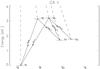 |
Fig. 1 Term diagram of the Ca ii model atom. The continuum is not shown. Energy levels (horizontal lines), bound-bound transitions (solid) and bound-free transitions (dashed). |
3.3. Magnesium
We use a three-level plus continuum model atom, including the ground state, the upper levels of the h & k lines and the continuum. Energy levels and oscillator strengths are from the NIST database, collisional excitation rates are from Sigut & Pradhan (1995), collisional ionization from Seaton’s semi-empirical formula (Allen 1964, p. 42) and photoionization cross-sections are from the Opacity Project1. The abundance is taken from Asplund et al. (2009). The h & k lines are computed assuming PRD.
4. Cooling from lines and continua
The basic cooling process is an electron impact excitation followed by a radiative deexcitation. If this photon escapes the atmosphere, the corresponding energy has been taken out of the thermal pool which corresponds to radiative cooling. In the corona these processes are the dominant ones: collisional excitation followed by radiative deexcitation with the photon escaping. Collisional de-excitation and absorption of photons (radiative excitation) are insignificant in comparison. This is often called the coronal approximation.
In the chromosphere we have a much more complex situation with all rates playing a role. In strong lines most of the photons emitted are immediately absorbed in the same transition but the collisional destruction probability is often very low and the photon may escape after a very large number of scattering events. We may also have photons absorbed in one line (e.g., Lyman-β) escaping in another transition (e.g., H-α). A full description of these processes entails solving the transfer equations coupled with the non-LTE rate equations (or statistical equilibrium equations if rates are assumed to be instantaneous).
We here choose to describe the net effect as a combination of three factors that need to be determined empirically from our simulations: (1) the optically thin radiative loss function (that gives the energy loss from the total generation of local photons in the absence of absorption per atom in the ionization stage of consideration (H i, Ca ii and Mg ii)), (2) the probability that this energy escapes from the atmosphere and (3) the fraction of atoms in the given ionization stage: 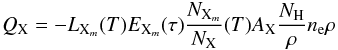 (1)where QX is the radiative heating (positive Q) or cooling (negative Q) per volume from element X (in our case H, Ca and Mg), LXm(T) is the optically thin radiative loss function as function of temperature, T, per electron, per particle of element X in ionization stage m, EXm(τ) is the escape probability as function of some depth parameter τ,
  is the fraction of element X that is in ionization stage m, AX is the abundance of element X,
  is the number of hydrogen particles per gram of stellar material, which is a constant for a given set of abundances (=4.407 × 10²³ for the solar abundances of Asplund et al. 2009), ne is the electron number density and ρ is the mass density.
The optically thin radiative loss function is equal to the collisional excitation rate in the coronal approximation and is then only a function of temperature. In the chromosphere this is not the case but the hope is that we may still write a radiative loss function as function of temperature only. We expect various routes between the levels (rather than a collisional excitation in one transition followed by a radiative deexcitation in the same transition) but as long as collisional de-excitation rates are small we expect the total collisional excitation from the ground state to be equal to the radiative losses:
Assume a gas where 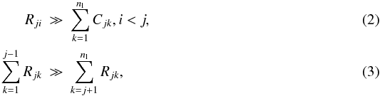 here Rji is the radiative rate coefficient from bound level j to i and Cjk the collisional rate coefficient from level j to k and nl is the number of energy levels of the atom. These assumptions imply that an excited atom will nearly always fall back to its ground state through one or more radiative transitions. Hence, photon absorption will always be followed by one or more radiative deexcitations, and the gas cannot absorb energy from the radiation field. The only way to lose energy from the gas through a bound-bound transition is through a collisional excitation followed by one or more radiative deexcitations. All energy of the initial excitation is then emitted as radiation and thermal energy is converted into radiation.
Therefore, as long as Eqs. (2) − (3) hold, the radiative losses LXm due to lines of atoms of species X in ionization stage m, per atom in ionization stage m per electron, is given by 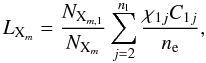 (4)where NXm,1 is the population density in the ground state of element X, ionization stage m, χ1j is the energy difference between the ground state (level 1) and level j. Collisions with electrons are dominant under typical chromospheric conditions and
  and therefore also LXm will be a function of temperature only (apart from the factor
  which is close to one). There are therefore reasons to believe that we may write the optically thin loss function as a function of temperature only. In Sect. 4.1 we will use our numerical simulations to deduce such relations and compare them with the total collisional excitation from the ground state (Eq. (4)).
In the chromosphere not all photons will escape the atmosphere. We parametrize this with the escape probability function EXm in Eq. (1). In Sect. 4.2 we use our simulations to calculate this escape probability empirically.
We complete the recipe by determining in Sect. 4.3 the factor in Eq. (1): the fraction of hydrogen, calcium and magnesium that resides in H i, Ca ii and Mg ii.
4.1. Optically thin radiative loss function
From the RADYN simulation we calculate the total radiative losses as the sum of the net downward radiative rates multiplied with the energy difference of the transition, summed over all bound-bound transitions and the Lyman-continuum transition (the other continuum transitions get thin low down in the atmosphere and their influence on the energy balance can be taken into account in a multi-group opacity approach).
Figure 2 shows the probability density function (PDF) of the total radiative losses per neutral hydrogen atom per electron as function of temperature for the RADYN simulation2. We exclude the startup phase of the first 1000 s of the simulation and only include points above 1.7 Mm height to avoid most points where the escape probability is small. For temperatures above 10 kK the relation is very tight and the PDF is close to the total excitation curve. Below 10 kK we have a larger spread, both because this part includes points with a low escape probability and because the approximations (Eqs. (2) − (3)) start to break down. At low temperatures, the optical depth in the Lyman transitions builds up quickly when integrating downwards in the atmosphere and only the uppermost of these points have an escape probability close to one. To account for points with low escape probability we therefore take the upper envelope as the adopted optically thin radiative loss function.
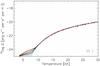 |
Fig. 2 Probability density function of the radiative losses in lines and the Lyman-continuum of H i in the RADYN test atmosphere as function of temperature for points above 1.7 Mm height. The curves give the adopted fit (red) and the total collisional excitation according to Eq. (4) (blue). |
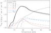 |
Fig. 3 Fit to the optically thin cooling per electron per hydrogen particle (thick solid), contributions from Lyman-α (thin black solid), Lyman-β (dashed), Lyman-γ (dot-dashed), H-α (red), Lyman-continuum (blue) and optically thin radiative losses from other elements than hydrogen (thick dotted) as function of temperature. |
Figure 3 shows the various contributions to the radiative cooling in hydrogen, this time per electron per hydrogen atom (and not per neutral hydrogen atom) to have a normalization similar to the one used for coronal optically thin radiative losses. In most of the temperature range, the Lyman-α transition dominates with at most 20% coming from other transitions (where Lyman-β and the Lyman-continuum are the most important ones). At the low temperature end, the Lyman-continuum starts to contribute and H-α eventually dominates below 7 kK. The hydrogen optically thin radiation dominates over contributions from other elements below 32 kK.
Figures 4, 5 show the probability density function of the total radiative losses per singly ionized calcium and magnesium atom, respectively, as function of temperature for the Bifrost simulation. This cooling was computed in detail using the radiative transfer code Multi3d (Leenaarts & Carlsson 2009) assuming statistical equilibrium and plane-parallel geometry with each column in the snapshot treated as an independent 1D atmosphere.
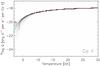 |
Fig. 4 Probability density function of the radiative losses in lines of Ca ii as function of temperature in the Bifrost test atmosphere for points above 1.3 Mm height. The curves give the adopted fit (red) and the total collisional excitation according to Eq. (4) (blue). |
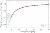 |
Fig. 5 Probability density function of the radiative losses in lines of Mg ii as function of temperature in the Bifrost test atmosphere for points above 1.3 Mm height. The curves give the adopted fit (red) and the total collisional excitation according to Eq. (4) (blue). |
The probability density function is close to the total collisional excitation curve for both Ca ii and Mg ii. In the case of Ca ii this may be a bit surprising at first glance. The Ca ii 3d 2D doublet is metastable and we do not include transitions from it to the ground state. This implies Eq. (2) does not hold. However, for typical chromospheric electron densities, gas temperatures and radiation temperatures in the infrared triplet the following relation holds:  (5)This means that an atom in a Ca ii 3d 2D state is much more likely to get radiatively excited to one of the Ca ii 4p 2P states than to move to another level through collisions. Therefore, transition chains starting with collisional excitation from the ground state to a metastable level typically go through a number of radiative transitions, and ultimately end in the ground state through a spontaneous emission from a Ca ii 4p 2P state. The original collision energy is then lost from the gas and Eq. (4) still holds. However, net collisional rates between the excited levels give a larger spread and also radiative losses that sometimes are smaller than the total collisional excitation from the ground state. In contrast to the case of hydrogen, the spread is thus not caused by optical depth effects and hence we take the average of the values for our fits rather than the upper envelope. At the lowest temperatures we also get points with radiative heating (not visible in the logarithmic plots) and the fits make a sharp dip downwards. See Sect. 5 for a discussion of radiative heating.
4.2. Escape probability
The assumption that all collisional excitations lead to emitted photons breaks down in the chromosphere, where increased mass density leads to increased probability of absorption of photons and collisional deexcitation. Once radiative excitation processes come into play we have many more possible routes in the statistical equilibrium. To fully account for these processes we have to solve the coupled radiative transfer equations and non-LTE rate equations. Instead, we calculate an empirical escape probability from the ratio of the actual cooling as obtained from a detailed radiative transfer computation and the optically thin cooling function determined in Sect. 4.1. Ideally we would like to tabulate this escape probability as a function of optical depth in the lines. Since we are dealing with the total cooling over a number of lines, there is no single optical depth scale to be chosen. For Ca ii and Mg ii we choose to tabulate the escape probability as a function of column mass. The rationale behind this choice is that the optical depth in the resonance lines is proportional to column mass as long as the ionization stage under consideration is the majority species. This is the case for both Ca ii and Mg ii, as shown in Sect. 4.3, in the region of the atmosphere where the optical depth is significant. Another advantage with the choice of column mass is that it is easy to calculate from the fundamental variables in a snapshot of an MHD simulation. For hydrogen the situation is different. The Lyman lines get optically thin in the lower part of the transition region where hydrogen gets ionized. In the 1D simulation used for calculating the empirical coefficients, the transition region stays at a constant column mass. On a column mass scale, the hydrogen escape probability would then be a very steep function. Instead, we need to use a depth-variable that is proportional to the neutral hydrogen column density. We use the total column density of neutral hydrogen multiplied with the constant 4 × 10-14 cm2 which gives a depth-variable that is close to the optical depth at line center of Lyman-α. The escape probability is high to rather high optical depths, because of the very large scattering probability in the Lyman transitions.
The escape probability depends in a complicated way on the density, electron density, temperature and local radiation field. We expect it to be close to unity at low column mass density, and to go to zero at large column mass density.
In order to derive an empirical relation we calculate the average (over time for the RADYN simulation and over space for the Bifrost snapshot) actual cooling and the average cooling according to the optically thin cooling function determined in Sect. 4.1 as function of the chosen depth-scale. We adopt this ratio as the empirical escape probability as function of depth.
Figure 6 shows the probability density function of the empirical escape probability as function of approximate optical depth at Lyman-α line center together with the adopted relation. Figures 7 and 8 show the probability density function of the empirical escape probability as function of column mass for Ca ii and Mg ii together with the adopted relation.
Note that the adopted relations are not the averages of the points shown in Figs. 6 − 8 but the ratio between the average of the actual cooling and the average of the optically thin cooling such that points with large cooling get larger weight. The adopted fit may therefore look like a poor representation of the PDFs of Figs. 6–8. If these figures had only included the points with the largest cooling, the correspondence would have been more obvious.
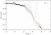 |
Fig. 6 Probability density function of the empirical escape probability as function of approximate optical depth at Lyman-α line center and the adopted fit (red). Only points with a cooling above 5 × 10⁹ erg s-1 g-1 are included and the startup phase of the simulation (first 1000 s) has been excluded. |
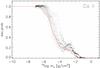 |
Fig. 7 Probability density function of the empirical escape probability as function of column mass for Ca ii and the adopted fit (red). Only points with a a cooling above 5 × 10⁸ erg s-1 g-1 are included. |
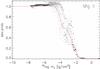 |
Fig. 8 Probability density function of the empirical escape probability as function of column mass for Mg ii and the adopted fit (red). Only points with a a cooling above 5 × 10⁸ erg s-1 g-1 are included. |
4.3. Ionization fraction
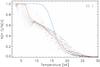 |
Fig. 9 Probability density function of the fraction of neutral H atoms as function of temperature in the RADYN test atmosphere between heights of 0.5 Mm and 2.0 Mm after the initial 1000 s. Curves show the adopted fit to the PDF (red), and the coronal approximation (blue). |
In Sects. 4.1–4.2 we derived expressions for the radiative losses per atom in the relevant ionization stage per electron. In order to convert these losses to actual losses per volume, the fraction of atoms in the ionization stage under study (H i, Ca ii and Mg ii) must be known. In general this quantity is a function of the electron density, temperature, radiation field, and, in case of small transition rates, the history of the atmosphere.
Neither Saha ionization equilibrium nor coronal equilibrium are valid in the chromosphere. Therefore no quick physics-based recipe exists that gives the ionization fraction. Fortunately, in our 1D and 2D test atmospheres, the ionization fraction as function of temperature shows a rather small spread around an average value and an empirical fit to these values gives a reasonable approximation. We also computed fits as function of temperature and electron density. As the ionization fraction is relatively insensitive to the electron density these two-parameter fits do not yield a significantly better approximation and we settle for relations as function of temperature only.
Figure 9 shows the probability density function of the fraction of H i, as function of temperature. There is a certain spread around the adopted fit which reflects the fact that the hydrogen ionzation is also a function of the history of the atmosphere. It is also clear that the coronal approximation gives a rather poor fit to the simulation data for temperatures below 30 kK.
Figure 10 shows the same relation for Ca ii. The points are rather close to the fitting function except for some points below 10 kK where an unusually strong radiation field may lead to a lower fraction of Ca ii for some columns of the atmosphere. The best fit curve lies between the coronal approximation curve for a six-level atom (green curve) and the one for a two-level atom (blue curve). The reason the coronal approximation for the six-level atom fails is that an overpopulation of the meta-stable levels drives an upward radiative net rate in the infrared triplet violating the approximation of no upward radiative rates in the coronal approximation. In the limit where this upward rate is much larger than the downward rate we recover the two-level approximation.
Figure 11 shows the ionization balance of Mg ii. The points are very close to the fitting curve over the full range of the simulation.
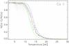 |
Fig. 10 Probability density function of the fraction of Ca atoms in the form of Ca ii as function of temperature in the Bifrost test atmosphere between heights of 0.5 Mm and 2.0 Mm. Curves show the adopted fit to the PDF (red), the coronal approximation (green) and the coronal approximation with a two-level atom (blue). |
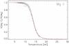 |
Fig. 11 Probability density function of the fraction of Mg atoms in the form of Mg ii as function of temperature in the Bifrost test atmosphere between heights of 0.5 Mm and 2.0 Mm. Curves show the adopted fit to the PDF (red), and the coronal approximation (blue). |
5. Radiative heating
In the preceding section we deduced recipes to describe the radiative cooling in transitions of H i, Ca ii and Mg ii. In the cool phases of the chromosphere the atmosphere can be heated by radiation in the same transitions.
The total radiative heating rate (radiative flux divergence) is given by 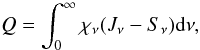 (6)where χν is the opacity, Jν is the mean intensity and Sν is the source function. Assuming a two-level atom and neglecting stimulated emission we have the following relations
 ![Mathematical equation: \begin{eqnarray} &&\chi_\nu=N_{{\rm X}_{m,i}}\alpha_0\phi_\nu=\frac{N_{{\rm X}_{m,i}}}{N_{{\rm X}_m}} \alpha_0\phi_\nu\frac{N_{{\rm X}_m}}{N_{\rm X}}A_{\rm X}\frac{N_{\rm H}}{\rho}\rho \\[2mm] &&S_\nu=\epsilon B_\nu + (1-\epsilon)J_\nu \\[2mm] &&\epsilon=\frac{C_{ji}}{A_{ji}+C_{ji}}\approx\frac{C_{ji}}{A_{ji}}=f(T)n_{\rm e}, \end{eqnarray}](/articles/aa/full_html/2012/03/aa18366-11/aa18366-11-eq45.png) where NXm,i is the population density of the lower level i, α0 is a constant, φν is the normalized absorption profile of the line, ϵ is the collisional destruction probability, Bν is the Planck function, Cji is the collisional deexcitation probability, Aji is the Einstein coefficient for spontaneous emission, f(T) is a function of temperature and the other terms have the same meaning as in Eq. (1). Inserting into Eq. (6) we get
where NXm,i is the population density of the lower level i, α0 is a constant, φν is the normalized absorption profile of the line, ϵ is the collisional destruction probability, Bν is the Planck function, Cji is the collisional deexcitation probability, Aji is the Einstein coefficient for spontaneous emission, f(T) is a function of temperature and the other terms have the same meaning as in Eq. (1). Inserting into Eq. (6) we get 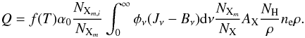 (10)This equation resembles Eq. (1);
  is a function of temperature in LTE, Jν is constant with height in the optically thin regime such that
  is a function of temperature (but also a function of the source function where Jν thermalizes). At larger optical depths, Jν approaches Bν and the integral behaves similarly to the escape probability E(τ) in Eq. (1). Although there are many approximations involved, the similarity to Eq. (1) leads us to adopt the same functional form for the heating as we have done for the cooling. We thus just use the previous fits also when LX(T) is negative (corresponding to heating) and adopt for simplicity the same escape probability function.
To test the applicability of this scheme we plotted the probability density function of the radiative losses (positive) and gains (negative) in the Bifrost test atmosphere, divided by the empirically defined escape probability, as function of temperature. The results are shown in Fig. 12 for CaII and Fig. 13 for MgII. The figures show that there is a fairly large spread in the losses/gains at low temperatures. For Ca ii we adopt a fit that gives gains below ~4 kK, for Mg ii we choose zero gains/losses below ~5 kK.
Heating in hydrogen transitions is mainly due to absorption of Lyman-α photons produced by a nearby source (a strong shock or the transition region). This is illustrated in Fig. 14, where there is heating due to Ly-α photons caused by the emission at 10log mc = −5.2. Such behaviour cannot be modeled with a simple local equation as Eq. (10) so we choose to set the losses and gains for hydrogen to zero below ~4 kK.
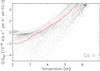 |
Fig. 12 Probability density function of the radiative losses in lines of Ca ii divided by the empirically determined escape probability as function of temperature in the Bifrost test atmosphere for points above 0.3 Mm height. The red curve gives the adopted fit. |
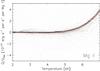 |
Fig. 13 Probability density function of the radiative losses in lines of Mg ii divided by the empirically determined escape probability as function of temperature in the Bifrost test atmosphere for points above 0.3 Mm height. The red curve gives the adopted fit. |
6. Comparison between detailed solution and recipes
We have now derived fits for the three factors that enter into the radiative cooling: the optically thin radiative loss function, the escape probability and the ionization fraction. To test the accuracy with which we can approximate the cooling calculated from the detailed solution of the non-LTE rate equations we here compare the detailed solution with our recipe. Since the detailed solution from a given test atmosphere has been used to derive the fits we here use different snapshots for this comparison (a different timeseries calculated with RADYN for hydrogen and a snapshot at a much later time calculated with Bifrost for calcium and magnesium).
Figure 14 shows the cooling ( − Q) as a function of column mass for hydrogen at a time in the RADYN simulation when there is a shock in the chromosphere. The detailed cooling is dominated by Lyman-α in the shock but with a significant contribution also from H-α. Behind the shock (larger column mass), H-α dominates the cooling. The total cooling is well approximated by our recipe. In front of the shock (smaller column mass) there is heating by absorption of Lyman-α photons. This heating is not accounted for in the recipe.
Figures 15 and 16 show the average cooling as function of height in the Bifrost test atmosphere. Since hydrogen cooling cannot be properly calculated in the Bifrost atmosphere we only show the recipe result for hydrogen (and use these values also for the calculation of the total detailed cooling) in order to show the relative importance of the three elements. It is clear that the recipes reproduce the average cooling very well. Hydrogen dominates in the upper chromosphere and transition region while magnesium dominates the cooling in the mid and lower chromosphere with equally strong calcium cooling at some heights. Note that this average cooling varies very much from snapshot to snapshot depending on the location of shocks in the atmosphere. These figures should thus only be used to compare the detailed solution with the approximate one and not as pictures of the mean chromospheric energy balance.
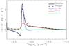 |
Fig. 14 Cooling as function of column mass from hydrogen transitions at t = 3170 s in the RADYN simulation. Total cooling from the detailed calculation (black solid), from the recipes (black dashed), Lyman-α (blue), H-α (red) and the Lyman continuum (green). |
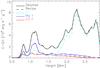 |
Fig. 15 Average cooling as function of height in the Bifrost test atmosphere. Total cooling (black), H i (turquoise), Mg ii (blue) and Ca ii (red). According to the detailed calculations (solid) and according to the recipes (dashed). |
7. Heating from incident radiation field
Part of the optically thin radiative losses from the corona escapes outwards, but an equal amount of energy is emitted towards the sun and is absorbed in the chromosphere where it contributes to radiative heating. Most of this radiation is absorbed in the continua of neutral helium and neutral hydrogen. If one assumes the coronal ionization equilibrium is only dependent on temperature, then the frequency-integrated coronal losses per volume (positive Q means heating, as before) are given by 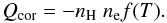 (11)Here f(T) is a positive function dependent on temperature only that can be pre-computed and tabulated from atomic data. The emissivity associated with this loss is
  (12)Because the coronal radiative losses are integrated over frequency one has to choose a single representative opacity to compute the absorption. A decent choice is to use the opacity at the ionization edge of the ground state of neutral helium (denoted by α). The opacity χ is then given by
 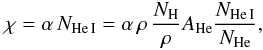 (13)where NHe I is the number density of neutral helium, NHe is the number density of helium, AHe is the abundance of helium relative to hydrogen, NH is the total number density of hydrogen particles and
  is a constant dependent on the abundances. The quantity NHe I/NHe can be pre-computed from a calibration computation as is done for H, Ca and Mg in Sect. 4.3.
The most accurate method for computing the absorption of coronal radiation in the chromosphere is to compute the 3D radiation field resulting from the coronal emissivity and the absorption using the radiative transfer equation: 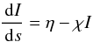 (14)with I the intensity and s the geometrical path length along a ray. The solution can be computed using standard long or short characteristics techniques in decomposed domains (Heinemann et al. 2006; Hayek et al. 2010). Once the intensity is known the heating rate can be directly computed as
  (15)with Ω the solid angle.
The method described above is accurate, but slow. A faster method can be obtained by treating each column in the MHD simulation as a plane-parallel atmosphere and assuming that at each location either η or χ is zero. For each column all quantities then become only a function of height z and Eq. (15) reduces to  (16)with μ the cosine of the angle with respect to the vertical.
If we furthermore assume the emitting region is located on top of the absorbing region, we can ignore rays that point outward from the interior of the star in the integral of Eq. (16). The intensity that impinges on the top of the absorbing region for inward pointing rays is simply the integral of the emissivity along the z-axis from the top (zt) to the bottom (zb) of the computational domain, weighted with the inverse of μ to account for slanted rays  (17)Now that we have computed the incoming intensity that impinges on the top of the absorbing region we can compute the intensity at all heights from the solution to the transfer equation with zero emissivity:
  (18)The vertical optical depth τ is computed from the top of the computational domain:
  (19)The integrals in Eqs. (17) and (19) can both be computed efficiently in parallel and need to be computed only once, independent of the number of μ-values in the angle discretization.
The method gives inaccurate results if the assumption of coronal emission above chromospheric absorption fails. This happens for example when a cool finger of chromospheric gas protrudes slanted into the corona.
Figure 17 shows a comparison of the 3D and the fast 1D method. The top panel shows the coronal emissivity η. It is mostly smooth with occasional very large peaks close to the transition region (red curve). The emissivity for gas colder than 30 kK (below the red curve) is negligible.
The second panel shows the angle-averaged radiation field computed in 3D (J3D in Eq. (15)). The radiation field is fairly smooth as it is determined by an average of the emissivity throughout the corona.
The middle panel shows the angle-averaged radiation field treating each column as a plane-parallel atmosphere (J1D in Eq. (16)). Here it is far from smooth. The radiation field is high in columns with a large integrated emissivity, as indicated by the green and red vertical stripes. Note that there is cool gas located above coronal gas around (x,z) = (8,3) Mm. Here the radiation field is highest at the top and decreases downward, while the emissivity panel shows that the emission is mainly coming from the coronal gas located below the cool finger.
The fourth panel shows the 3D heating rate. The heating rate is non-zero only below the red curve, validating our assumption for the fast 1D method of separate absorbing and emitting regions. It is fairly smooth, with quite some heating in the cool bubble around (x,z) = (4,4) Mm, caused by coronal radiation coming in from the sides. The bottom panel shows the 1D heating rate. It shows large extrema in columns with large integrated emissivity, and is less smooth than the 3D heating. Because it is computed column-by-column, it cannot include the sideways radiation in the cool bubble as indicated by the low heating rate there compared to the 3D case. However, its overall appearance is quite similar to the 3D heating rate.
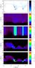 |
Fig. 17 Comparison of the 1D and 3D method for computing chromospheric heating due to absorption of coronal radiation. All panels show a vertical slice through a snapshot of a three-dimensional radiation-MHD simulation performed with Bifrost. The red curve is located at a gas temperature of 30 000 K and indicates the location of the transition zone. All brightness ranges have been clipped to bring out variation at low values of the displayed quantities. Panels, from top to bottom: coronal emissivity η; angle-averaged radiation field computed in 3D; angle-averaged radiation field computed in 1D: heating rate per mass with 3D radiation: heating rate per mass with 1D radiation. Note that the 3D radiation field is computed using the full 3D volume, not only this 2D slice. |
Figure 18 compares the horizontally averaged heating rate as function of height computed from the 1D recipe with the 3D heating rate. The recipe is always within 15% of the 3D heating. Part of this difference is caused by numerical errors because the strong coronal emission close to the transition region is only barely resolved on the grid used in the simulation.
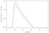 |
Fig. 18 Horizontally-averaged radiative heating by absorption of coronal radiation as function of height in the 3D Bifrost test atmosphere from the detailed 3D computation (solid) and from the 1D recipe (dashed). |
8. Conclusions
We have shown that the radiative cooling in the solar chromosphere by hydrogen lines, the Lyman continuum, the H and K and infrared triplet lines of singly ionized calcium, and the h and k lines of singly ionized magnesium can be expressed fairly accurately as easily computed functions. These functions are the product of an optically thin emission (dependent on temperature), an escape probability (dependent on column mass) and an ionization fraction (dependent on temperature). While at any given location in the atmosphere our recipe might deviate from the true cooling, it is nevertheless remarkably accurate when averaged over time and/or space as indicated by Figs. 14 − 16.
We have shown that radiative heating can be approximated with the same functional form as radiative cooling. However, the heating is strongly dependent on the details of the local radiation field and absorption profile, so the recipe is not nearly as accurate for heating as it is for cooling. Our detailed computations show that radiative heating in the h and k lines of Mg ii is negligible, and small, but present, for the lines of Ca ii. Heating due to hydrogen is mainly through absorption of Lyman-α photons next to the transition region or shock waves. This effect cannot be modeled with our recipes.
In addition we have presented a simple method to compute chromospheric heating by absorption of coronal radiation. This method approximates the diffuse component of the heating, but yields localized spots of spurious intense heating owing to the column-by-column approach that prevents spreading of radiation. It reproduces the spatially averaged heating very well. Given its simplicity and speed it is a good alternative to the slower, more accurate method that requires a formal solution of the transfer equation.
The recipes have been developed for solar chromospheric conditions. For sunspot conditions or for other stars it would be necessary to redo the semi-empirical fits using detailed radiative transfer calculations applied to appropriate simulations.
This figure, and many of the following figures, are not scatterplots but 2D histograms normalized for each x-axis bin. The darkness at a y-axis bin is thus a measure of the probability of finding an atmospheric point at this particular y-value given that it is in the x-axis bin.
Acknowledgments
This research was supported by the Research Council of Norway through the grant “Solar Atmospheric Modelling” and through grants of computing time from the Programme for Supercomputing. J.L. acknowledges financial support from the European Commission through the SOLAIRE Network (MTRN-CT-2006-035484) and from the Netherlands Organization for Scientific Research (NWO).
References
- Abbett, W. P., & Hawley, S. L. 1999, ApJ, 521, 906 [NASA ADS] [CrossRef] [Google Scholar]
- Allen, C. W. 1964, Astrophysical Quantities, 2nd edn. (London: Athlone Press) [Google Scholar]
- Allred, J. C., Hawley, S. L., Abbett, W. P., & Carlsson, M. 2005, ApJ, 630, 573 [NASA ADS] [CrossRef] [Google Scholar]
- Allred, J. C., Hawley, S. L., Abbett, W. P., & Carlsson, M. 2006, ApJ, 644, 484 [NASA ADS] [CrossRef] [Google Scholar]
- Anderson, L. S., & Athay, R. G. 1989, ApJ, 346, 1010 [NASA ADS] [CrossRef] [Google Scholar]
- Arnaud, M., & Rothenflug, R. 1985, A&AS, 60, 425 [NASA ADS] [Google Scholar]
- Asplund, M., Grevesse, N., Sauval, A. J., & Scott, P. 2009, ARA&A, 47, 481 [NASA ADS] [CrossRef] [Google Scholar]
- Bard, S., & Carlsson, M. 2010, ApJ, 722, 888 [NASA ADS] [CrossRef] [Google Scholar]
- Bashkin, S., & Stoner, J. O. 1975, Atomic energy levels and Grotrian Diagrams – Vol. 1: Hydrogen I – Phosphorus XV, Vol. 2: Sulfur I – Titanium XXII (Amsterdam: North-Holland Publ. Co.) [Google Scholar]
- Burgess, A., & Chidichimo, M. C. 1983, MNRAS, 203, 1269 [NASA ADS] [CrossRef] [Google Scholar]
- Burgess, A., & Tully, J. A. 1992, A&A, 254, 436 [NASA ADS] [Google Scholar]
- Carlsson, M., & Stein, R. F. 1992, ApJ, 397, L59 [NASA ADS] [CrossRef] [Google Scholar]
- Carlsson, M., & Stein, R. F. 1994, in Proc. Mini-Workshop on Chromospheric Dynamics, ed. M. Carlsson (Oslo: Institute of Theoretical Astrophysics), 47 [Google Scholar]
- Carlsson, M., & Stein, R. F. 1995, ApJ, 440, L29 [NASA ADS] [CrossRef] [Google Scholar]
- Carlsson, M., & Stein, R. F. 1997, ApJ, 481, 500 [Google Scholar]
- Carlsson, M., & Stein, R. F. 2002, ApJ, 572, 626 [NASA ADS] [CrossRef] [Google Scholar]
- Cheng, J. X., Ding, M. D., & Carlsson, M. 2010, ApJ, 711, 185 [NASA ADS] [CrossRef] [Google Scholar]
- Fossum, A., & Carlsson, M. 2005, Nature, 435, 919 [NASA ADS] [CrossRef] [PubMed] [Google Scholar]
- Fossum, A., & Carlsson, M. 2006, ApJ, 646, 579 [NASA ADS] [CrossRef] [Google Scholar]
- Gudiksen, B., Carlsson, M., Hansteen, V. H., et al. 2011, A&A, 531, A154 [NASA ADS] [CrossRef] [EDP Sciences] [Google Scholar]
- Hayek, W., Asplund, M., Carlsson, M., et al. 2010, A&A, 517, A49 [NASA ADS] [CrossRef] [EDP Sciences] [Google Scholar]
- Heinemann, T., Dobler, W., Nordlund, Å., & Brandenburg, A. 2006, A&A, 448, 731 [NASA ADS] [CrossRef] [EDP Sciences] [Google Scholar]
- Janev, R. K., Langer, W. D., & Evans, K. 1987, Elementary processes in hydrogen-helium plasmas – Cross sections and reaction rate coefficients (Berlin: Springer) [Google Scholar]
- Jin, J., & Church, D. A. 1993, Phys. Rev. Lett., 70, 3213 [NASA ADS] [CrossRef] [PubMed] [Google Scholar]
- Johnson, L. C. 1972, ApJ, 174, 227 [NASA ADS] [CrossRef] [Google Scholar]
- Judge, P. G., Carlsson, M., & Stein, R. F. 2003, ApJ, 597, 1158 [NASA ADS] [CrossRef] [Google Scholar]
- Kašparová, J., Varady, M., Heinzel, P., Karlický, M., & Moravec, Z. 2009, A&A, 499, 923 [NASA ADS] [CrossRef] [EDP Sciences] [Google Scholar]
- Klein, R. I., Kalkofen, W., & Stein, R. F. 1976, ApJ, 205, 499 [NASA ADS] [CrossRef] [Google Scholar]
- Klein, R. I., Stein, R. F., & Kalkofen, W. 1978, ApJ, 220, 1024 [NASA ADS] [CrossRef] [EDP Sciences] [Google Scholar]
- Kupka, F., Piskunov, N., Ryabchikova, T. A., Stempels, H. C., & Weiss, W. W. 1999, A&AS, 138, 119 [NASA ADS] [CrossRef] [EDP Sciences] [MathSciNet] [PubMed] [Google Scholar]
- Leenaarts, J., & Carlsson, M. 2009, in ASP Conf. Ser., 415, ed. B. Lites, M. Cheung, T. Magara, J. Mariska, & K. Reeves, 87 [Google Scholar]
- Leenaarts, J., Carlsson, M., Hansteen, V., & Rutten, R. J. 2007, A&A, 473, 625 [NASA ADS] [CrossRef] [EDP Sciences] [Google Scholar]
- Leenaarts, J., Carlsson, M., Hansteen, V., & Gudiksen, B. V. 2011, A&A, 530, A124 [NASA ADS] [CrossRef] [EDP Sciences] [Google Scholar]
- Meléndez, M., Bautista, M. A., & Badnell, N. R. 2007, A&A, 469, 1203 [NASA ADS] [CrossRef] [EDP Sciences] [Google Scholar]
- Menzel, D. H., & Pekeris, C. L. 1935, MNRAS, 96, 77 [NASA ADS] [Google Scholar]
- Milkey, R. W., & Mihalas, D. 1973, ApJ, 185, 709 [NASA ADS] [CrossRef] [Google Scholar]
- Piskunov, N. E., Kupka, F., Ryabchikova, T. A., Weiss, W. W., & Jeffery, C. S. 1995, A&AS, 112, 525 [NASA ADS] [Google Scholar]
- Rammacher, W., & Ulmschneider, P. 2003, ApJ, 589, 988 [NASA ADS] [CrossRef] [Google Scholar]
- Shull, J. M., & van Steenberg, M. 1982, ApJS, 48, 95 [NASA ADS] [CrossRef] [Google Scholar]
- Sigut, T. A. A., & Pradhan, A. K. 1995, J. Phys. B At. Mol. Phys., 28, 4879 [NASA ADS] [CrossRef] [Google Scholar]
- Sugar, J., & Corliss, C. 1985, Atomic energy levels of the iron-period elements: Potassium through Nickel (Washington: American Chemical Society) [Google Scholar]
- Theodosiou, C. E. 1989, Phys. Rev. A, 39, 4880 [NASA ADS] [CrossRef] [Google Scholar]
- Tobiska, W. K. 1991, J. Atm. Terr. Phys., 53, 1005 [Google Scholar]
- Vernazza, J. E., Avrett, E. H., & Loeser, R. 1981, ApJS, 45, 635 [NASA ADS] [CrossRef] [Google Scholar]
- Vriens, L., & Smeets, A. H. M. 1980, Phys. Rev. A, 22, 940 [NASA ADS] [CrossRef] [Google Scholar]
- Wahlstrom, C., & Carlsson, M. 1994, ApJ, 433, 417 [NASA ADS] [CrossRef] [Google Scholar]
- Wedemeyer-Böhm, S., & Carlsson, M. 2011, A&A, 528, A1 [NASA ADS] [CrossRef] [EDP Sciences] [Google Scholar]
All Figures
|
Fig. 1 Term diagram of the Ca ii model atom. The continuum is not shown. Energy levels (horizontal lines), bound-bound transitions (solid) and bound-free transitions (dashed). |
| In the text | |
|
Fig. 2 Probability density function of the radiative losses in lines and the Lyman-continuum of H i in the RADYN test atmosphere as function of temperature for points above 1.7 Mm height. The curves give the adopted fit (red) and the total collisional excitation according to Eq. (4) (blue). |
| In the text | |
|
Fig. 3 Fit to the optically thin cooling per electron per hydrogen particle (thick solid), contributions from Lyman-α (thin black solid), Lyman-β (dashed), Lyman-γ (dot-dashed), H-α (red), Lyman-continuum (blue) and optically thin radiative losses from other elements than hydrogen (thick dotted) as function of temperature. |
| In the text | |
|
Fig. 4 Probability density function of the radiative losses in lines of Ca ii as function of temperature in the Bifrost test atmosphere for points above 1.3 Mm height. The curves give the adopted fit (red) and the total collisional excitation according to Eq. (4) (blue). |
| In the text | |
|
Fig. 5 Probability density function of the radiative losses in lines of Mg ii as function of temperature in the Bifrost test atmosphere for points above 1.3 Mm height. The curves give the adopted fit (red) and the total collisional excitation according to Eq. (4) (blue). |
| In the text | |
|
Fig. 6 Probability density function of the empirical escape probability as function of approximate optical depth at Lyman-α line center and the adopted fit (red). Only points with a cooling above 5 × 10⁹ erg s-1 g-1 are included and the startup phase of the simulation (first 1000 s) has been excluded. |
| In the text | |
|
Fig. 7 Probability density function of the empirical escape probability as function of column mass for Ca ii and the adopted fit (red). Only points with a a cooling above 5 × 10⁸ erg s-1 g-1 are included. |
| In the text | |
|
Fig. 8 Probability density function of the empirical escape probability as function of column mass for Mg ii and the adopted fit (red). Only points with a a cooling above 5 × 10⁸ erg s-1 g-1 are included. |
| In the text | |
|
Fig. 9 Probability density function of the fraction of neutral H atoms as function of temperature in the RADYN test atmosphere between heights of 0.5 Mm and 2.0 Mm after the initial 1000 s. Curves show the adopted fit to the PDF (red), and the coronal approximation (blue). |
| In the text | |
|
Fig. 10 Probability density function of the fraction of Ca atoms in the form of Ca ii as function of temperature in the Bifrost test atmosphere between heights of 0.5 Mm and 2.0 Mm. Curves show the adopted fit to the PDF (red), the coronal approximation (green) and the coronal approximation with a two-level atom (blue). |
| In the text | |
|
Fig. 11 Probability density function of the fraction of Mg atoms in the form of Mg ii as function of temperature in the Bifrost test atmosphere between heights of 0.5 Mm and 2.0 Mm. Curves show the adopted fit to the PDF (red), and the coronal approximation (blue). |
| In the text | |
|
Fig. 12 Probability density function of the radiative losses in lines of Ca ii divided by the empirically determined escape probability as function of temperature in the Bifrost test atmosphere for points above 0.3 Mm height. The red curve gives the adopted fit. |
| In the text | |
|
Fig. 13 Probability density function of the radiative losses in lines of Mg ii divided by the empirically determined escape probability as function of temperature in the Bifrost test atmosphere for points above 0.3 Mm height. The red curve gives the adopted fit. |
| In the text | |
|
Fig. 14 Cooling as function of column mass from hydrogen transitions at t = 3170 s in the RADYN simulation. Total cooling from the detailed calculation (black solid), from the recipes (black dashed), Lyman-α (blue), H-α (red) and the Lyman continuum (green). |
| In the text | |
|
Fig. 15 Average cooling as function of height in the Bifrost test atmosphere. Total cooling (black), H i (turquoise), Mg ii (blue) and Ca ii (red). According to the detailed calculations (solid) and according to the recipes (dashed). |
| In the text | |
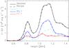 |
Fig. 16 As Fig. 15 but for the low-mid chromosphere. |
| In the text | |
|
Fig. 17 Comparison of the 1D and 3D method for computing chromospheric heating due to absorption of coronal radiation. All panels show a vertical slice through a snapshot of a three-dimensional radiation-MHD simulation performed with Bifrost. The red curve is located at a gas temperature of 30 000 K and indicates the location of the transition zone. All brightness ranges have been clipped to bring out variation at low values of the displayed quantities. Panels, from top to bottom: coronal emissivity η; angle-averaged radiation field computed in 3D; angle-averaged radiation field computed in 1D: heating rate per mass with 3D radiation: heating rate per mass with 1D radiation. Note that the 3D radiation field is computed using the full 3D volume, not only this 2D slice. |
| In the text | |
|
Fig. 18 Horizontally-averaged radiative heating by absorption of coronal radiation as function of height in the 3D Bifrost test atmosphere from the detailed 3D computation (solid) and from the 1D recipe (dashed). |
| In the text | |
Current usage metrics show cumulative count of Article Views (full-text article views including HTML views, PDF and ePub downloads, according to the available data) and Abstracts Views on Vision4Press platform.
Data correspond to usage on the plateform after 2015. The current usage metrics is available 48-96 hours after online publication and is updated daily on week days.
Initial download of the metrics may take a while.