| Issue |
A&A
Volume 539, March 2012
|
|
|---|---|---|
| Article Number | A107 | |
| Number of page(s) | 12 | |
| Section | The Sun | |
| DOI | https://doi.org/10.1051/0004-6361/201118345 | |
| Published online | 02 March 2012 | |
The non-Maxwellian continuum in the X-ray, UV, and radio range⋆
1
Department of Astronomy, Physics of the Earth and MeteorologyFaculty of
Mathematics, Physics and Informatics, Comenius University,
Mlynská Dolina F2,
842 48
Bratislava,
Slovak Republic
e-mail: This email address is being protected from spambots. You need JavaScript enabled to view it.
2
Astronomical Institute of the Academy of Sciences of the Czech
Republic, Fričova
298, 251 65
Ondřejov, Czech
Republic
Received:
27
October
2011
Accepted:
27
January
2012
Abstract
Aims. We investigate the X-ray, UV, and also the radio continuum arising from plasmas with a non-Maxwellian distribution of electron energies. The two investigated types of distributions are the κ- and n-distributions.
Methods. We derived analytical expressions for the non-Maxwellian bremsstrahlung and free-bound continuum spectra. The spectra were calculated using available cross-sections. Then we compared the bremsstrahlung spectra arising from the different bremsstrahlung cross-sections that are routinely used in solar physics.
Results. The behavior of the bremsstrahlung spectra for the non-Maxwellian distributions is highly dependent on the assumed type of the distribution. At flare temperatures and hard X-ray energies, the bremsstrahlung is greatly increased for κ-distributions and exhibits a strong high-energy tail. With decreasing κ, the maximum of the bremsstrahlung spectrum decreases and moves to higher wavelengths. In contrast, the maximum of the spectra for n-distributions increases with increasing n, and the spectrum then falls off very steeply with decreasing wavelength. In the millimeter radio range, the non-Maxwellian bremsstrahlung spectra are almost parallel to the thermal bremsstrahlung. Therefore, the non-Maxwellian distributions cannot be detected by off-limb observations made by the ALMA instrument. The free-bound continua are also highly dependent on the assumed type of the distribution. For n-distributions, the ionization edges disappear and a smooth continuum spectrum is formed for n ≧ 5. Opposite behavior occurs for κ-distributions where the ionization edges are in general significantly enhanced, with details depending on κ and T through the ionization equilibrium. We investigated how the non-Maxwellian κ-distributions can be determined from the observations of the continuum and conclude that one can sample the low-energy part of the distribution from the continuum.
Key words: Sun: X-rays, gamma rays / Sun: radio radiation / radiation mechanisms: non-thermal / atomic processes
Appendix A is available in electronic form at http://www.aanda.org
© ESO, 2012
1. Introduction
Assuming a Maxwellian distribution of particle energies is most widely used to describe the astrophysical plasma. This has its roots in the Boltzmann-Gibbs statistical mechanics, which is in turn based on the assumption that the collisions in the studied plasma are sufficiently frequent to attain the thermal equilibrium. However, the assumption of the Maxwellian distribution has been challenged in the past decades in a wide variety of astrophysical environments, ranging from laboratory plasmas to planetary magnetospheres, the solar wind, and even galaxies (e.g., Dalla & Ljepojevic 1997; Maksimovic et al. 1997a,b; Viñas et al. 2000; Petkaki et al. 2003; Mauk et al. 2004; Leubner 2004a,b, 2005; Maksimovic et al. 2005; Ryu et al. 2007, 2009; Gaelzer et al. 2008; Nieves-Chinchilla & Viñas 2008; Dialynas et al. 2009; Prokhorov 2009; Prokhorov et al. 2009; Le Chat et al. 2009; Pierrard 2009; Pierrard & Lazar 2010; Pierrard et al. 2011; Livadiotis & McComas 2010; Lu et al. 2010, 2011; Leitner et al. 2011).
In solar physics, on which we focus here, departures from the equilibrium Maxwellian distribution occur every time particles are accelerated, e.g., in flares, where high-energy tails are ubiquitous (Petkaki & MacKinnon 2007, 2011; Zharkova & Gordovskyy 2006; Veronig et al. 2010; Zharkova et al. 2010, 2011; Fletcher et al. 2011; Holman et al. 2011). Apart from that, departures from Maxwellian distributions can occur at low plasma densities if there are strong gradients of temperature and density, i.e., in the transition region (e.g., Owocki & Scudder 1983; Ljepojevic & MacNiece 1988; Scudder 1992; Pinfield et al. 1999; Dzifčáková & Kulinová 2011), in conditions where the mean energy can change (Collier 2004), i.e., during plasma heating. These processes commonly result in the formation of power-law, high-energy tails. However, changes in the bulk of the distribution function were also reported during flares (Seely et al. 1987; Dzifčáková et al. 2008; Kulinová et al. 2011).
The non-Maxwellian distributions are often represented in an analytical parametric form, described by several free parameters, one of which is usually connected to the temperature or mean energy, i.e., the second moment of the distribution function. In the spectroscopy of solar corona and flares, one such class of parametric distributions are the κ-distributions. They were first proposed by Vasyliunas (1968) and are characterized by the parameter κ, which gives the degree of departure from the Maxwellian distribution and also the asymptotic slope of the high-energy tail of the distribution (see Eq. (1) in Sect. 2). Their presence in the flaring plasma was studied by Kašparová & Karlický (2009). These authors showed that the κ-distributions can explain the thin-target bremsstrahlung spectrum of some coronal sources in partially occulted flares. Dzifčáková & Kulinová (2010) proposed a method of diagnosing κ-distributions based on line ratios observed by Hinode/EIS (Culhane et al. 2007) and SPIRIT spectrometers (Zhitnik et al. 2005). They found that the Fe xi – Fe xii line spectra during a flare observed by the SPIRIT spectrometer can be explained by the κ-distribution with κ = 2. This finding was not supported by a differential emission measure (DEM) analysis, however, and is thus questionable. In contrast to this, Dzifčáková & Kulinová (2011) showed that the transition region Si iii spectra can be explained by the κ-distribution with κ ranging from κ = 7 in the active region to κ = 13 in the coronal hole. This diagnostics is valid also for the plasma characterized by DEMs with varying steepness at temperatures where the Si iii lines are formed. The κ-distributions were also observed in the solar wind at distances of 1–2.3 AU (e.g., Maksimovic et al. 1997a,b; Zouganelis 2008; Le Chat et al. 2009, 2011; Pierrard 2011). Pierrard et al. (1999) and Vocks & Mann (2003) showed that the distribution function with a high-energy tail in the solar wind can indeed originate in the open magnetic structures at the base of the quiet solar corona through resonant interaction of electrons with the whistler-waves. The formation of κ-distributions in the closed coronal loop geometry was studied by Vocks et al. (2008). Formation of κ-distributions by ion-sound turbulence and beam-plasma interaction has been studied e.g. by Rhee et al. (2006) and Yoon et al. (2006). A comprehensive review on κ-distribution in space plasmas can be found in Pierrard & Lazar (2010).
Another parametric distribution is the n-distribution, invoked to explain the observed ratios of dielectronic to allowed lines during solar flares (Seely et al. 1987; Dzifčáková et al. 2008; Kulinová et al. 2011). These works report increased intensities of the X-ray Fe or Si dielectronic satellite lines with respect to allowed lines of a nearby He-like ion of the same element. This increase occurs only during the impulsive phase of the observed flares, coincides with the presence of electron beams inferred from radio bursts (Kulinová et al. 2011), and most importantly, cannot be explained by emission from a multithermal Maxwellian plasma (Dzifčáková et al. 2008). Moreover, Kulinová et al. (2011) combined the X-ray observations made by the RESIK spectrometer (Sylwester et al. 2005) with the RHESSI (Lin et al. 2002) observations of energies down to 4 keV to show that not only the presence of n-distributions increase the goodness-of-fit in terms of χ2, but that the emission measure associated with the plasma with n-distribution dominates over the contribution from the thermal component. In the range of a few keV, which corresponds to the excitation energy of the dielectronic satellites, the n-distribution can be mimicked by the Maxwellian distribution with a velocity drift (Karlický et al. 2012).
The influence of the non-Maxwellian distributions on the ionization equilibrium in the solar corona was studied by e.g. Anderson et al. (1996); Dzifčáková (1998, 2002) and Wannawichian et al. (2003), and on excitation equilibrium by Dzifčáková (2000, 2006); Dzifčáková & Tóthová (2007) and Dzifčáková & Mason (2008). The main result of these works is that changes in the processes of ionization and excitation are significant and lead to changes in the predicted line intensities. This on one hand allows us to determine the presence of the non-Maxwellian distributions from the observations, but also leads to changes in the total radiative losses (Dudík et al. 2011) that possibly affect the energy balance in the solar corona. Changes in the line intensities also lead to different responses of TRACE EUV filters (Dudík et al. 2009).
Continua related to the non-Maxwellian distributions were studied for decades mainly in the hard X-ray and radio range. There, the power-law distributions were usually assumed to be responsible for the observed emission processes, such as bremsstrahlung in the hard X-ray range (e.g., Brown 1971; Lin & Hudson 1971; Holman et al. 2003; Krucker & Lin 2008; Krucker et al. 2008; Asai et al. 2009; Warmuth et al. 2009; Veronig et al. 2010; Kurt et al. 2010; Zharkova et al. 2010; Guo et al. 2011; Kontar et al. 2011) or gyrosynchrotron emission in the radio range (e.g., Dulk 1985; Zhou & Karlický 1994; Kuznetsov et al. 2011). Yasnov & Karlický (2009) presented an inverse method to determine the characteristics of the electron power-law tail distribution in radio bursts. Using this method, Yasnov & Karlický (2010) showed that the presence of power-law tails can indeed be inferred from radio observations. Bremsstrahlung emission produced by the electron κ and n-distributions was considered in the analyses of RHESSI hard X-ray solar flare spectra by Kašparová & Karlický (2009) and Kulinová et al. (2011).
In this paper, we present calculations of the free-free (bremsstrahlung) and free-bound continua for the κ- and n-distributions. We evaluate these continua in the X-ray, UV, and even radio spectral range. With the calculation of line intensities already available, the calculations of the free-free and free-bound continua in this paper represent the completion of the spectral synthesis for these non-Maxwellian distributions.
The organization of this paper is as follows. The non-Maxwellian distributions and their properties are summarized in Sect. 2. The calculation of the bremsstrahlung spectra is carried out in Sect. 3, with Sect. 3.2 focusing on comparison of various bremsstrahlung cross-sections used in solar physics. The calculation of the free-bound continuum is presented in Sect. 4, where we also propose a method to diagnose the non-Maxwellian distributions in flare plasma using the continuum only. Our conclusions are summarized in Sect. 5.
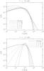 |
Fig. 1 κ- and n-distributions as functions of ℰ for T or τ = 107 K. |
2. The non-Maxwellian distributions
The term “non-Maxwellian electron distribution” refers to any distribution of electron
energies ℰ other than the Maxwellian distribution. The two widely used parametric
distributions are the κ-distributions
fκ(ℰ)dℰ (e.g., Owocki & Scudder 1983; Livadiotis
& McComas 2009) and the n-distributions
fn(ℰ)dℰ (e.g., Seely et al. 1987; Kulinová et al.
2011), defined respectively as  where
where
 =
=  and ℬn =
  are normalization constants,
kB ≈ 1.38 × 10⁻¹⁶ erg s-1 is the
Boltzmann constant, and κ ∈ ⟨3/2,∞),
n ∈ ⟨1,∞), and T are the parameters
of the distributions. We note that the κ-distribution can be defined in
several ways. Here, in Eq. (1), we use the
κ-distribution of the second kind (Livadiotis & McComas 2009). The Maxwellian distribution is a special case
recovered for κ-distribution with κ → ∞. It also
corresponds to the n-distribution with n = 1. The
κ- and n-distributions for various κ
and n are plotted in Fig. 1.
are normalization constants,
kB ≈ 1.38 × 10⁻¹⁶ erg s-1 is the
Boltzmann constant, and κ ∈ ⟨3/2,∞),
n ∈ ⟨1,∞), and T are the parameters
of the distributions. We note that the κ-distribution can be defined in
several ways. Here, in Eq. (1), we use the
κ-distribution of the second kind (Livadiotis & McComas 2009). The Maxwellian distribution is a special case
recovered for κ-distribution with κ → ∞. It also
corresponds to the n-distribution with n = 1. The
κ- and n-distributions for various κ
and n are plotted in Fig. 1.
The interpretation of T as the temperature is valid only for κ-distributions, where the mean energy ⟨ℰ⟩κ = (3/2)kBT is independent of κ and thus has the same value as for the Maxwellian distribution. For more details on the definition of temperature for the κ-distributions in the framework of nonextensive statistics (Tsallis 1988, 2009), the reader is referred to the work of Livadiotis & McComas (2009).
The mean energy ⟨ℰ⟩n for the n-distributions
depends on n,
⟨ℰ⟩n = (n/2 + 1)kBT.
For the n-distributions, the pseudo-temperature τ was
defined by Dzifčáková (1998) (3)so that
⟨ℰ⟩n = (3/2)kBτ,
giving τ the same meaning for n-distributions as
T for the Maxwellian or κ-distributions. To keep the
notation consistent with previously published papers, we will use T
and τ as the independent variables for the κ- and
n-distributions, respectively.
(3)so that
⟨ℰ⟩n = (3/2)kBτ,
giving τ the same meaning for n-distributions as
T for the Maxwellian or κ-distributions. To keep the
notation consistent with previously published papers, we will use T
and τ as the independent variables for the κ- and
n-distributions, respectively.
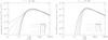 |
Fig. 2 Bremsstrahlung spectra for κ-distributions (left) and n-distributions (right). The spectra must be multiplied by the nenH factor to obtain the actual emissivity. |
 |
Fig. 3 Predicted quiet-Sun (T = 1 MK) bremsstrahlung spectra for κ-distributions (left) and n-distributions (right) at radio wavelengths. The spectra must be multiplied by the nenH factor to obtain the actual emissivity. |
3. The non-Maxwellian bremsstrahlung
3.1. Non-Maxwellian bremsstrahlung spectrum
The expressions for bremsstrahlung spectrum (wavelength-dependent emissivity) for the
non-Maxwellian κ- and n-distributions is obtained from
Eqs. (12) and (13) of Dudík et al. (2011) by
dropping the wavelength integral  where
w = hc/λkBT = E/kBT
is the scaled photon energy, λ is the wavelength, E the
corresponding photon energy, h ≈ 6.62 × 10⁻²⁷ erg s is the
Planck constant, and c ≈ 3 × 1010 cm s-1 is the
speed of light. The gff is the free-free Gaunt factor. The
value of C depends on the assumed chemical composition, ionization
balance, and electron density
where
w = hc/λkBT = E/kBT
is the scaled photon energy, λ is the wavelength, E the
corresponding photon energy, h ≈ 6.62 × 10⁻²⁷ erg s is the
Planck constant, and c ≈ 3 × 1010 cm s-1 is the
speed of light. The gff is the free-free Gaunt factor. The
value of C depends on the assumed chemical composition, ionization
balance, and electron density 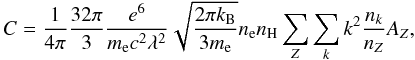 (6)where
k is the ionization degree of an ion of the element with proton number
Z whose abundance is AZ.
The Pff has units of
[erg cm-3 s-1 sr-1 Å-1]. The bremsstrahlung
spectrum for the non-Maxwellian κ- and n-distributions
is shown in Fig. 2 for
T = 107 K and τ = 107 K,
respectively. We used the Gaunt factor gff calculated by Sutherland (1998) and the ionization equilibria for the
κ- and n-distributions calculated by Dzifčáková (2002) and Dzifčáková (1998), respectively. For the Maxwellian (n = 1)
distribution, the ionization equilibrium of Mazzotta
et al. (1998) was used. The bremsstrahlung spectrum is only weakly dependent on
the ionization balance, because most of the contribution to emissivity comes from the most
abundant element, hydrogen (Sect. 3.2, Fig. 4). We used the coronal abundances for
Z ≦ 30 elements based on the works of Feldman et al. (1992), Grevesse & Sauval
(1998), and Landi et al. (2002), compiled
in the CHIANTI (Dere et al. 1997, 2009) sun_coronal_ext.abund file. We
note that the Gaunt factor gff is in the work of Sutherland (1998) scaled by the ionization energy and
thus depends on the ionization stage k and proton number
Z of the given element. Thus, the integration in Eqs. (4) and (5) with the Sutherland gff must be performed for
each ion separately.
(6)where
k is the ionization degree of an ion of the element with proton number
Z whose abundance is AZ.
The Pff has units of
[erg cm-3 s-1 sr-1 Å-1]. The bremsstrahlung
spectrum for the non-Maxwellian κ- and n-distributions
is shown in Fig. 2 for
T = 107 K and τ = 107 K,
respectively. We used the Gaunt factor gff calculated by Sutherland (1998) and the ionization equilibria for the
κ- and n-distributions calculated by Dzifčáková (2002) and Dzifčáková (1998), respectively. For the Maxwellian (n = 1)
distribution, the ionization equilibrium of Mazzotta
et al. (1998) was used. The bremsstrahlung spectrum is only weakly dependent on
the ionization balance, because most of the contribution to emissivity comes from the most
abundant element, hydrogen (Sect. 3.2, Fig. 4). We used the coronal abundances for
Z ≦ 30 elements based on the works of Feldman et al. (1992), Grevesse & Sauval
(1998), and Landi et al. (2002), compiled
in the CHIANTI (Dere et al. 1997, 2009) sun_coronal_ext.abund file. We
note that the Gaunt factor gff is in the work of Sutherland (1998) scaled by the ionization energy and
thus depends on the ionization stage k and proton number
Z of the given element. Thus, the integration in Eqs. (4) and (5) with the Sutherland gff must be performed for
each ion separately.
In the hard X-ray range, the spectrum is very sensitive to the high-energy tail of the distribution (Fig. 2). Even a very weak enhancement of this tail can greatly enhance the bremsstrahlung spectrum. For instance, for κ = 34, the bremsstrahlung emissivity at λ = 1 Å for T = 107 K is about a factor of 7.5 higher than the corresponding emissivity for the Maxwellian distribution. For κ = 5 the increase is by a factor of ~800, and for κ = 2 by a factor of ~6000. We note that for κ-distributions, the integrand in Eq. (4) falls slowly with increasing y for low values of κ. This is because the increased number of electrons in the high-energy tail of the κ-distribution is able to produce enhanced bremsstrahlung emission at short wavelengths.
For the n-distributions, the spectrum in the short-wavelength range decreases steeply (Fig. 2, right). We note here that the n-distribution can explain the dielectronic line intensities in flares. However, the n-distribution is a parametric distribution that describes well only the bulk of the distribution function during flares (Dzifčáková et al. 2011). In particular, the n-distributions do not contain the high-energy tail observed commonly during flares (e.g., Asai et al. 2009; Veronig et al. 2010; Zharkova et al. 2010; Guo et al. 2011). This high-energy tail then dominates the bremsstrahlung spectrum at the X-ray wavelengths and corresponding photon energies of tens of keV. Therefore, the decrease of the bremsstrahlung spectrum at these wavelengths predicted by Eq. (5) is not relevant for flare observations. On the other hand, the bremsstrahlung spectrum predicted by the n-distributions describes well the bremsstrahlung spectrum observed at longer wavelengths, which corresponds to the photon energies down to 4 keV (Kulinová et al. 2011).
Near its maximum, the bremsstrahlung spectra for both non-Maxwellian distributions mimic the shape of the distribution. With decreasing κ, the emissivity peak decreases and moves to longer wavelengths. The n-distributions show an opposite effect, with an increased peak of the emissivity (Fig. 2). In the long-wavelength range, the behavior of the bremsstrahlung spectrum for non-Maxwellian distributions essentially copies the Maxwellian bremsstrahlung spectrum. In the λ = 0.1–10 cm range, the curves are almost parallel (Fig. 3). Therefore, the non-Maxwellian distributions are not detectable by e.g. the off-limb observations of the solar corona with the ALMA radio instrument (Karlický et al. 2011). Interpreting the observed radio spectra under the assumption of e.g. a κ-distribution would only yield lower brightness temperature of the radio source compared to the one derived under the assumption of the Maxwellian (thermal) distribution. We note that Chiuderi & Chiuderi Drago (2004) studied the microwave radio emission originating in a model of the transition region characterized by a DEM and a κ-distribution. These authors calculated the radio transfer equation and obtained lower brightness temperatures compared to the Maxwellian distribution for all frequencies. However, their results are not directly comparable to ours, since we calculate only the emissivity from a unit volume of an optically thin, isothermal coronal plasmas, and not a radio transfer equation from the entire model atmosphere.
 |
Fig. 4 Comparison of the bremsstrahlung spectra calculated using the approach outlined in Sect. 3.1 (labeled “CHIANTI”) and the RHESSI SSW tree. Full line denotes the ratio of the purely hydrogen bremsstrahlung, Pff CHIANTI/Pff RHESSI, computed using the “CHIANTI” approach and the RHESSI software. Ratios of the bremsstrahlung due to all elements with Z ≦ 30 to the purely hydrogen bremsstrahlung, Pff/Pff,H, for the coronal abundances (dashed line) and photospheric abundances (dotted line) computed according to Eqs. (4)–(6) are compared to the multiplicative factor of 1.44 used in the RHESSI SSW (horizontal gray line). |
3.2. Comparison of the bremsstrahlung cross-sections used in solar physics
In Sect. 3.1, we studied the wavelength range extending over several spectral domains: hard X-rays, soft X-rays, and radio wavelengths. The SolarSoftWare (SSW) provides several methods to compute theoretical bremsstrahlung spectra at X-ray energies. These methods can be found in e.g. the CHIANTI and XRAY packages of the SSW tree. Because at the X-ray range the bremsstrahlung emission is strongly dependent on the assumed type of non-Maxwellian distribution, we now proceed to compare the methods available in the SSW tree. We tested their compatibility mainly in the ranges close to or outside their common use, i.e., between soft and hard X-ray energies (~0.1−10 keV). The crucial element is the bremsstrahlung cross-section or the free-free Gaunt factor.
In the soft X-ray range, the approach based on the Gaunt factors is adopted, whereas the
hard X-ray photon emission is usually calculated in terms of cross-sections. The Gaunt
factor is the multiplicative correction of the classical Kramers cross-section (e.g. Phillips et al. 2008), so one can write
 (7)where
σff(E,ℰ) is the cross-section differential
in the photon energy E in units of cm2 per unit
E,
α = 2πe2/hc
is the fine-structure constant, and
r0 = e2/mec2
is classical electron radius.
(7)where
σff(E,ℰ) is the cross-section differential
in the photon energy E in units of cm2 per unit
E,
α = 2πe2/hc
is the fine-structure constant, and
r0 = e2/mec2
is classical electron radius.
The Gaunt factors of Sutherland (1998) used in this paper are based on Karzas & Latter (1961) work, who assumed non-relativistic electrons moving in a pure Coulomb field of an unscreened nucleus. In the hard X-ray range, e.g. for the analysis of RHESSI data, the non-relativistic bremsstrahlung cross-section given in the first Born approximation (Haug 1997) for an unscreened nucleus is used (see brm_bremcross.pro routine in the SSW tree). This cross-section is sufficiently accurate up to semirelativistic electron energies (i.e., ℰ ≲ 300 keV) for low-Z nuclei, e.g., hydrogen and helium.
In order to make the comparison simple, we focused on the bremsstrahlung on the most abundant element – hydrogen and energies up to ~100 keV. The Sutherland (1998) and Haug (1997) hydrogen bremsstrahlung cross-sections agree to within about 5% in a broad range of initial electron energies, generally from ~10-3 to ~102 keV, and corresponding photon energies ~10-3 to ~102 keV, although separate ranges with a stronger deviation occur.
The comparison of the bremsstrahlung spectra calculated using the Haug (1997) and Sutherland (1998) cross-sections are presented in Fig. 4. Here, the comparison is shown for a representative sample of the κ- and n-distributions considered in this paper. The Pff CHIANTI and Pff,RHESSI corresponds to the bremsstrahlung from the purely hydrogen plasma (i.e., AZ = 0 for Z ≧ 2) calculated using Eqs. (4)–(6) and the RHESSI SSW, respectively. The spectra usually agree to within 10% in the photon energy range of E ≈ 10-2–3 × 101 keV for all distributions considered in this paper. The deviation rises at higher E for n-distributions. However, in this range, the bremsstrahlung spectrum for the n-distributions decreases very steeply by more than five orders of magnitude (Fig. 2, right), resulting in an increase of the relative numerical error.
In RHESSI SSW (f_thin_kappa.pro, f_thin_ndistr.pro, and also routines for power-law tails), the contribution from Z ≧ 2 elements is incorporated by using a multiplication factor of (1.2)2 = 1.44 to the hydrogen bremsstrahlung. Figure 4 shows the comparison of this predicted total bremsstrahlung with the one computed using Eqs. (4)–(6) using both the coronal and photospheric abundances for Z ≦ 30 elements as implemented in CHIANTI. We note that the contribution from higher-Z elements is expected to be negligible because of their very low abundances.
As shown in Fig. 4, for T or τ = 10 MK, and κ = 2 and 5, and n = 1 and 11, the multiplication factor is a good approximation only at very low photon energies E < 10-1 keV, with details depending on the type of the distribution because of the changes in the ionization equilibrium entering C in Eq. (6). A better approximation for coronal abundances for E < 1 keV would be a multiplication factor of 1.5. At higher E, deviations from the value of 1.44 occur. The situation is worst for n = 11. However, we note again that at photon energies of tens of keV, the bremsstrahlung spectrum for n-distributions decreases of very steeply for the assumed T or τ = 10 MK. Therefore, the deviation from the value of 1.44 due to the contribution of other elements will have only a small effect on the general behavior of the bremsstrahlung spectrum at these energies.
Our result that the Sutherland (1998) and Haug (1997) cross-sections and the corresponding bremsstrahlung spectra agree to within 5%, and 10%, respectively, is in contrast with the claim of Koch & Motz (1959) that the approach of non-relativistic Coulomb wave functions adopted for Sutherland’s Gaunt factors should not be valid for keV and higher initial electron energies.
We note that Seltzer & Berger (1986) tabulated a comprehensive set of bremsstrahlung cross-sections for electron energies 1 keV–1 GeV incident on neutral atoms with Z = 1−100. Those cross-sections are based on calculations by Pratt et al. (1977, 1981) who used a partial-wave method for screened nuclei. Seltzer & Berger (1986) extended the results by linear extrapolation to obtain the cross-section for hydrogen and also included bremsstrahlung produced in the field of atomic electrons. Taking the Seltzer & Berger (1986) cross-section only for atomic nucleus and ignoring the contribution of electron-electron bremsstrahlung produced in the field of atomic electrons yields agreement within the relative error of 5% with the Haug (1997) values in the ~1−50 keV range of initial electron energies (corresponding photon energies cover generally ~60% of the available range). However, the screening effects and the contribution of electron-electron bremsstrahlung produced in the field of atomic electrons, which are not included in Haug (1997) and Sutherland (1998), can be important for electron energies ℰ below 10 keV and always at low photon energies, i.e. E < 0.1ℰ (Seltzer & Berger 1986). We note that these effects are usually not considered in astrophysical applications. In the case of the Sun, this is because at coronal and flare temperatures hydrogen and helium are fully ionized and produce the greater part of the electron-ion bremsstrahlung. The contribution of other elements is directly proportional to their abundances (Eq. (6)). On the other hand, the screening effects can affect the bremsstrahlung produced in partially ionized hydrogen-helium plasma, e.g., in flare chromospheric footpoints. We also note that the contribution of electron-electron bremsstrahlung produced in the field of free electrons is important only at electron energies ℰ ≳ 200–300 keV (Haug 1975a,b; Kontar et al. 2007).
We are aware that a more general study of the free-free cross-sections including the screening effects and bremsstrahlung produced in the field of atomic electrons is needed. However, such a detailed study of the available cross-sections and their validity and applicability for astrophysical applications is out of the scope of this paper and is left for future work.
 |
Fig. 5 Free-bound spectra for κ-distributions (left column) and n-distributions (right column). The spectra must be multiplied by the nenH factor to obtain the actual emissivity. Two wavelength ranges are shown: λ = 0.1–1000 Å, same as in Fig. 2, to illustrate the general behavior (top row), and a close-up near the peak, λ = 3–10 Å (bottom row) to show the dependence of individual ionization edges on the shape of the distribution. |
 |
Fig. 6 Total continuum spectra, represented here by the sum of the contributions from bremsstrahlung and the free-bound continuum. Left: continuum for κ-distributions, right: continuum for the n-distributions. The spectra must be multiplied by the nenH factor to obtain the actual emissivity. |
4. The non-Maxwellian free-bound continuum
4.1. The free-bound continuum spectrum
The spectrum that arises from recombination transitions that in turn result in
k-times ionized ions of element Z with an electron on
an excited level i is given by (cf., derivation of Eq. (4.131) in Phillips et al. 2008)  (8)where
E = hc/λ = ℰ + Ii
is the energy of the emitted photon, Ii is
the ionization potential from the level i whose statistical weight is
gi, and
(8)where
E = hc/λ = ℰ + Ii
is the energy of the emitted photon, Ii is
the ionization potential from the level i whose statistical weight is
gi, and
 is the
ionization cross-section from the level i. Substituting the electron
distributions f(ℰ) from Eqs. (1) and (2), and summing through
all elements Z, their ions k and the excitation levels
i, the final expressions for the freebound continuum spectrum are
obtained
is the
ionization cross-section from the level i. Substituting the electron
distributions f(ℰ) from Eqs. (1) and (2), and summing through
all elements Z, their ions k and the excitation levels
i, the final expressions for the freebound continuum spectrum are
obtained  (9)for
the κ-distributions and
(9)for
the κ-distributions and 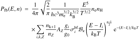 (10)for
the n-distributions. The calculated free-bound spectra are shown in Fig.
5. These spectra were calculated using the
ionization equilibrium files produced by Dzifčáková
(1998) and Dzifčáková (2002) and the
modified freebound.pro and freebound_ion.pro routines of
the CHIANTI package. The
cross-sections that are inserted into these routines are obtained from the works of Karzas & Latter (1961) and Verner & Yakovlev (1995). The modified routines
along with the ionization equilibrium files and other routines of the modification of
CHIANTI are available on demand from the authors.
(10)for
the n-distributions. The calculated free-bound spectra are shown in Fig.
5. These spectra were calculated using the
ionization equilibrium files produced by Dzifčáková
(1998) and Dzifčáková (2002) and the
modified freebound.pro and freebound_ion.pro routines of
the CHIANTI package. The
cross-sections that are inserted into these routines are obtained from the works of Karzas & Latter (1961) and Verner & Yakovlev (1995). The modified routines
along with the ionization equilibrium files and other routines of the modification of
CHIANTI are available on demand from the authors.
The most conspicuous feature is the disappearance of the ionization edges for n-distributions. This is because of the additional [(E − Ii)/kBT](n−1)/2 term in Eq. (10), which approaches zero for E → Ii. The short-wavelength side of the ionization edge then starts to be dominated by contributions of other ions. For example, for n = 3 the Mg xii edge is still visible as an abrupt change of the slope of the continuum (dotted line in Fig. 5, bottom right or Fig. 6, right). For n ≧ 5, the continuum is smooth without any noticeable local features.
On the other hand, the ionization edges are greatly increased for κ-distributions. Their general behavior is given by Eq. (9), but the details depend on κ and T through ionization equilibrium. While some of the ionization edges can be greatly increased for κ-distributions with given κ and T (e.g., Mg xii in Fig. 5, bottom left, for T = 107 K), others may be actually decreased at the same κ and T (e.g., Ni xxii and Fe xxii in the same image).
The relative height of the ionization edges with the type of the distribution reflects
the number of low-energy electrons that dominate the recombination processes. This is
because of the decrease of the cross-sections with the
increase of electron energy ℰ (e.g., Karzas &
Latter 1961). Thus, the rate of the radiative recombination is directly dependent
on the number of low-energy electrons, which is enhanced for
κ-distributions. On the other hand, there are very few low-energy
electrons for the n-distributions (Fig. 1), which results in the disappearance of the ionization edges for
n-distributions.
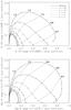 |
Fig. 7 Theoretical diagnostics plots for the κ-distributions from the ionization edges of Si and Mg. Top: ratios of the Si xiii and Si xiv edges to the total continuum at the wavelength of the edge. Bottom: the same as in top, but for Mg xi and Mg xii. The thin gray lines are isotherms connecting the points of constant log(T/K) for different κ. |
4.2. Diagnostics of the distribution from the continuum
Clearly, the heights of the ionization edges with respect to the total continuum can theoretically allow for diagnosing the type of the distribution. We note that here, the total continuum is represented by the sum of the contributions from bremsstrahlung and free-bound continuum (Fig. 6), because the two-photon continuum only has a negligible contribution (e.g., Phillips et al. 2008).
On one hand, the absence of ionization edges would immediately point to the presence of n-distributions. On the other hand, if the ionization edges do exist, their heights can be used to determine the presence of κ-distributions. As an example, we show the dependence of the height of the He-like and H-like ionization edges of Si and Mg on T and κ (Fig. 7). The height of the edge in Fig. 7 is measured relative to the total continuum at the wavelength of the edge, i.e., as the relative contribution of the photons emitted during the recombination process in a given ion to the local sum of the free-free and free-bound continua.
We note that using the He-like ions is advantageous, because they survive over a relatively wide temperature range, and an ionization edge of a corresponding H-like ion is nearby. However, the plots shown in Fig. 7 are only theoretical. This is because the ionization edge can in reality be overlapped by emission lines originating at similar temperatures. E.g., the Si xiii (λ = 5.086 Å) edge is located very close to a series of S xv lines, in particular to the 1s2 1S0 → 1s 2p 3P1 (λ = 5.067 Å) and 1s2 1S0 → 1s 2s 3S1 (λ = 5.101 Å) lines, whose contribution function has a maximum at log(T/K) = 7.1 for the Maxwellian distribution and 7.2 for the extreme non-Maxwellian case of κ = 2. On the other hand, the Si xiv edge at λ = 4.638 Å is, according to the CHIANTI database, located in a relatively uncrowded part of the spectrum. Because the relative height of this edge is always less than 0.11 for the Maxwellian distribution, this edge can be used to determine the maximum value of κ in e.g. the flaring plasma.
The Mg xi and Mg xii edges are more sensitive to the presence of the κ-distributions (Fig. 7bottom), but both these edges are overlapped by spectral lines. The Mg xii edge located at λ = 6.317 Å is obscured by the 1s2 1S0 → 1s 4p 1P1 (λ = 6.314 Å) transition in Al xiii as well as other Si xiiid transitions located less than 0.04 Å on both sides of the edge. The Mg xi edge at λ = 7.037 Å is located nearby the 1s 2S1/2 → 3p 2P3/2 (λ = 7.106 Å) transition in Mg xii, as well as several Si xiid and Ni xxvi transitions. Careful modeling of a high-resolution, high-quality spectrum would be needed to detect the κ-distributions from the Mg xi and Mg xii edges. This modeling would necessarily have to be accompanied by an EM-loci or DEM analysis (see e.g., Schmelz et al. 2009, 2011; Warren et al. 2011, for a recent application of these methods).
In a more general sense, the height of the ionization edges reflects the number of low-energy electrons in any electron energy distribution. If the true energy distribution in the observed plasma is unknown or time-dependent (e.g., due to instabilities, Karlický et al. 2012), the proposed diagnostic method can be used to sample the relative number of low-energy electrons in this distribution. To sample the higher energies in this unknown distribution, diagnostic methods involving lines formed at different energies (i.e., with different excitation treshholds) can be employed. Ratios of dielectronic to allowed emission lines even allow sampling discrete energies (e.g., Gabriel & Phillips 1979; Dzifčáková et al. 2008; Kulinová et al. 2011). The high-energy tail can be observed directly by e.g. RHESSI, taking the advantage of the bremsstrahlung emission. Combining the diagnostics from the continuum with diagnostics involving lines would form the basis of a method to sample any and the entire electron distribution in the flare plasma.
We also note that the height of the ionization edge can distinguish between the true n-distribution and the “moving Maxwellian” distribution (Maxwellian with a velocity drift, Karlický et al. 2012, Figs. 1–3 therein), which are very similar in the range of few keV, and therefore both can explain the observed intensities of dielectronic Si xiid lines during flares, but differ greatly in the low-energy end.
In Appendix A we present an application of the diagnostic method for κ-distributions to a more realistic scenario of a continuum spectrum emerging from a plasma that is mostly Maxwellian, but with the addition of a non-Maxwellian component.
5. Conclusions
We investigated the optically thin coronal and flare continuum spectrum caused by bremsstrahlung and recombination transitions arising from plasmas with non-Maxwellian electron κ- or n-distributions. The calculations of the non-Maxwellian continuum in this paper represent the completion of the spectral synthesis for non-Maxwellian distributions.
The general behavior of the bremsstrahlung spectrum for wavelengths shorter than the wavelength of the spectrum maximum is highly dependent on the assumed type of the distribution. Since the behavior of the spectrum is primarily influenced by the number of high-energy electrons, significant enhancement of the free-free continuum at flare temperatures and X-ray energies occur for κ-distributions. In contrast, the spectrum decreases very steeply for the n-distributions. For these distributions, the maximum of the bremsstrahlung spectrum is increased and shifted to shorter wavelengths, while for the κ-distributions, the maximum is decreased and shifted to longer wavelengths.
At millimeter radio wavelengths, corresponding to the ALMA range, the κ- and n-distributions are undetectable. The presence of these non-Maxwellian distributions would only affect the brightness temperature of the radio source.
The hydrogen bremsstrahlung spectrum calculated using the Sutherland (1998) free-free Gaunt factor is within 10% of the spectrum calculated using the Haug (1997) approach implemented in the RHESSI SolarSoftWare tree. For typical flare temperatures, the differences increase in the range of few tens of keV for n-distributions, but because the spectrum decreases very sharply for these energies, the resulting behavior of the spectrum would be influenced only weakly.
The height of the ionization edges in the free-bound continuum is also highly dependent on the assumed type of distributions. Because the height of the edges reflects the relative number of low-energy electrons, the edges increase greatly with decrease of κ, with details depending on temperature through the ionization equilibrium. The ionization edges disappear for n-distributions, resulting in a smooth free-bound continuum for n ≧ 5.
The height of the ionization edges can be used to derive the value of κ. We explored the diagnostic possibilities using He-like and H-like ions of Si and Mg. The diagnostics is difficult because of spectral lines in the immediate spectral neighborhood of the edges. Nevertheless, the Si xiv edge can still be used to detect the κ-distributions in flare plasma. Because the height of the ionization edges depends on the relative number of the low-energy electrons, they can provide a tool for sampling the low-energy end of the electron distribution that is otherwise not readily accessible from line spectra.
Online material
Appendix A: Is there a way to quantify the degree of departure of plasma from the Maxwellian distribution?
The diagnostic technique described in Sect. 4.2 provides a method to measure the κ of the distribution that governs the electrons in the plasma. In this appendix, we consider the case where the observed plasma is mostly Maxwellian. We demonstrate how the degree of departure from the purely Maxwellian plasma can then be quantified. To do this, we apply the diagnostic technique from Fig. 7 to the following case study.
We assume that the observed emission along the line-of-sight is originating in two emitting volumes. One of these volumes is characterized by a Maxwellian distribution, temperature T and the emission measure EM(Maxw). The other volume is characterized by a κ-distribution with a given κ, the same T, and a different EM(κ). The emerging continuum signal is then given by the sum of the contributions of the free-free and free-bound continua from these two volumes.
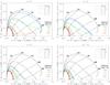 |
Fig. A.1 Determination of the apparent κ from the combination of a Maxwellian plasma and a plasma with a κ-distribution with known κ. The known κ is labeled in the title of each image in the panel. Black lines and their respective coding are the same as in Fig. 7. Colored lines denote the dependence of the relative height of the ionization edges on the emission measure ratio EM(Maxw)/EM(κ) = 10-2 (red), 10-1 (orange), 1 (green) and 10 (blue). Asterisks denote the points corresponding to log(T/K) = 6.8, 7.0, and 7.2. Except for the top left panel for κ = 2, these points are always close to the respective isotherms (gray lines). |
Then, using the diagnostic plots in Fig. 7 to determine κ leads, except at very low T, to higher apparent values of κ depending on the ratio EM(Maxw)/EM(κ) (Fig. A.1). For a plasma that is mostly Maxwellian, i.e., EM(Maxw)/EM(κ) ≪ 1, the diagnostics leads to almost Maxwellian plasma. That is, using the Si xiii and Si xiv edges for a combination of Maxwellian plasma and plasma with κ = 2, the height of the edges is consistent with Maxwellian plasma if EM(Maxw)/EM(κ) = 10-2 (red line in Fig. A.1top left). However, the apparent value of κ can be equal to ≈10 if the EM(Maxw)/EM(κ) is ten times higher, i.e., equal to 10-1 (orange line in Fig. A.1top left).
On the other hand, if the emission measure of the plasma with the κ-distribution is much greater than the EM(Maxw), then the diagnosed value of κ approaches the true value (Fig. A.1).
We can thus conclude that if the plasma has the same T, or at most a narrow DEM, any increase in the height of the ionization edge must be the consequence of the presence of κ-distributions.
We note here that the presented case study is fairly simple, because we assumed that the value of T is the same for the Maxwellian plasma and the plasma with a κ-distribution. Of course, the scenario can be complicated in many ways (e.g., diffferent T, or a multi-strand plasma characterized with a DEM and varying κ). In those cases, the diagnostics using only two ionization edges is clearly inappropriate and the observer would have to carefully check for the signatures of plasma multithermality, e.g., appearance of ionization edges or lines formed at higher or lower T.
We also note that if the Maxwellian and κ-distributed plasmas can be spatially resolved, the plot in Fig. 7 can be simply used for each spatial pixel separately and should lead to the correct results.
The same analysis as presented here could be also repeated for a combination of Maxwellian plasma and a plasma characterized with an n-distribution. However, then the ionization edges would be decreased with respect to the Maxwellian distribution, and therefore could prove to be much more difficult to be observed. For this reason, we chose to demonstrate the diagnostics using the κ-distributions.
Finally, we note that using RHESSI observations of the flare plasma, Kulinová et al. (2011) were able to resolve the contribution of the bresstrahlung produced by plasma with an n-distribution from the thermal component. This was possible because the bremsstrahlung from n-distributions manifests itself at energies of ≳4 keV, while the thermal component peaks at ≈7 keV. However, the closeness of these two components leads to large errors in determining n from RHESSI observations (Table A.7 in Kulinová et al. 2011).
Acknowledgments
This work was supported by Scientific Grant Agency, VEGA, Slovakia, Grant Nos. 1/0240/11, Grants Nos. 205/09/1705, 209/12/1652, and P209/12/0103 of the Grant Agency of the Czech Republic. J.D. also acknowledges support from Comenius University grant No. UK/57/2011. CHIANTI is a collaborative project involving the NRL (USA), RAL (UK), MSSL (UK), the Universities of Florence (Italy) and Cambridge (UK), and George Mason University (USA). It is a great spectroscopic database and software, and the authors are very grateful for its existence and availability.
References
- Anderson, S. W., Raymond, J. C., & van Ballegooijen, A. 1996, ApJ, 457, 939 [NASA ADS] [CrossRef] [Google Scholar]
- Asai, A., Nakajima, H., Shimojo, M., et al. 2009, ApJ, 695, 1623 [NASA ADS] [CrossRef] [Google Scholar]
- Brown, J. C. 1971, Sol. Phys., 18, 489 [NASA ADS] [CrossRef] [Google Scholar]
- Chiuderi, C., & Chiuderi Drago, F. 2004, A&A, 422, 331 [NASA ADS] [CrossRef] [EDP Sciences] [Google Scholar]
- Collier, M. R. 2004, Adv. Space Res., 33, 2108 [NASA ADS] [CrossRef] [Google Scholar]
- Culhane, J. L., Harra, L. K., James, A. M., et al. 2007, Sol. Phys., 243, 19 [Google Scholar]
- Dalla, S., & Ljepojevic, N. N. 1997, Phys. Plasmas, 4, 2052 [NASA ADS] [CrossRef] [Google Scholar]
- Dere, K. P., Landi, E., Mason, H. E., Monsignori Fossi, B. C., & Young, P. R. 1997, A&AS, 125, 149 [NASA ADS] [CrossRef] [EDP Sciences] [Google Scholar]
- Dere, K. P., Landi, E., Young, P. R., et al. 2009, A&A, 498, 915 [NASA ADS] [CrossRef] [EDP Sciences] [Google Scholar]
- Dialynas, K., Krimigis, S. M., Mitchell, D. G., et al. 2009, J. Geophys. Res., 114, A01212 [Google Scholar]
- Dudík, J., Kulinová, A., Dzifčáková, E., & Karlický, M. 2009, A&A, 505, 1255 [NASA ADS] [CrossRef] [EDP Sciences] [Google Scholar]
- Dudík, J., Dzifčáková, E., Karlický, M., & Kulinová, A. 2011, A&A, 529, A103 [NASA ADS] [CrossRef] [EDP Sciences] [Google Scholar]
- Dulk, G. A. 1985, ARA&A, 23, 169 [NASA ADS] [CrossRef] [Google Scholar]
- Dzifčáková, E. 1998, Sol. Phys., 178, 317 [NASA ADS] [CrossRef] [Google Scholar]
- Dzifčáková, E. 2000, Sol. Phys., 196, 113 [NASA ADS] [CrossRef] [Google Scholar]
- Dzifčáková, E. 2002, Sol. Phys., 208, 91 [NASA ADS] [CrossRef] [Google Scholar]
- Dzifčáková, E. 2006, Sol. Phys., 234, 243 [NASA ADS] [CrossRef] [Google Scholar]
- Dzifčáková, E., & Kulinová, A. 2010, Sol. Phys., 263, 25 [NASA ADS] [CrossRef] [Google Scholar]
- Dzifčáková, E., & Kulinová, A. 2011, A&A, 531, A122 [NASA ADS] [CrossRef] [EDP Sciences] [Google Scholar]
- Dzifčáková, E., & Mason, H. E. 2008, Sol. Phys., 247, 301 [NASA ADS] [CrossRef] [Google Scholar]
- Dzifčáková, E., & Tóthová, D. 2007, Sol. Phys., 240, 211 [NASA ADS] [CrossRef] [Google Scholar]
- Dzifčáková, E., Kulinová, A., Chifor, C., et al. 2008, A&A, 488, 311 [NASA ADS] [CrossRef] [EDP Sciences] [Google Scholar]
- Dzifčáková, E., Homola, M., & Dudík, J. 2011, A&A, 531, A111 [NASA ADS] [CrossRef] [EDP Sciences] [Google Scholar]
- Feldman, U., Mandelbaum, P., Seely, J. F., Doschek, G. A., & Gursky, H. 1992, ApJS, 81, 387 [NASA ADS] [CrossRef] [Google Scholar]
- Fletcher, L., Dennis, B. R., Hudson, H. S., et al. 2011, Space Sci. Rev., 159, 19 [NASA ADS] [CrossRef] [Google Scholar]
- Gabriel, A. H., & Phillips, K. J. H. 1979, MNRAS, 189, 319 [NASA ADS] [Google Scholar]
- Gaelzer, R., Ziebell, L. F., Viñas, A. F., Yoon, P. H., & Ryu, C.-M. 2008, ApJ, 677, 676 [NASA ADS] [CrossRef] [Google Scholar]
- Grevesse, N., & Sauval, A. J. 1998, Space Sci. Rev., 85, 161 [NASA ADS] [CrossRef] [Google Scholar]
- Guo, J., Liu, S., Fletcher, L., & Kontar, E. P. 2011, ApJ, 728, 4 [NASA ADS] [CrossRef] [Google Scholar]
- Haug, E. 1975a, Zeitschrift Naturforschung Teil A, 30, 1099 [Google Scholar]
- Haug, E. 1975b, Sol. Phys., 45, 453 [NASA ADS] [CrossRef] [Google Scholar]
- Haug, E. 1997, A&A, 326, 417 [NASA ADS] [Google Scholar]
- Holman, G. D., Sui, L., Schwartz, R. A., & Emslie, A. G. 2003, ApJ, 595, L97 [NASA ADS] [CrossRef] [Google Scholar]
- Holman, G. D., Aschwanden, M. J., Aurass, H., et al. 2011, Space Sci. Rev., 159, 107 [NASA ADS] [CrossRef] [Google Scholar]
- Karlický, M., Bárta, M., Dąbrowski, B. P., & Heinzel, P. 2011, Sol. Phys., 268, 165 [NASA ADS] [CrossRef] [Google Scholar]
- Karlický, M., Dzifčáková, E., & Dudík, J. 2012, A&A, 537, A36 [NASA ADS] [CrossRef] [EDP Sciences] [Google Scholar]
- Karzas, W. J., & Latter, R. 1961, ApJS, 6, 167 [NASA ADS] [CrossRef] [Google Scholar]
- Kašparová, J., & Karlický, M. 2009, A&A, 497, L13 [NASA ADS] [CrossRef] [EDP Sciences] [Google Scholar]
- Koch, H. W., & Motz, J. W. 1959, Rev. Mod. Phys., 31, 920 [NASA ADS] [CrossRef] [Google Scholar]
- Kontar, E. P., Emslie, A. G., Massone, A. M., et al. 2007, ApJ, 670, 857 [NASA ADS] [CrossRef] [Google Scholar]
- Kontar, E. P., Brown, J. C., Emslie, A. G., et al. 2011, Space Sci. Rev., 279 [Google Scholar]
- Krucker, S., & Lin, R. P. 2008, ApJ, 673, 1181 [NASA ADS] [CrossRef] [Google Scholar]
- Krucker, S., Battaglia, M., Cargill, P. J., et al. 2008, A&ARv, 16, 155 [Google Scholar]
- Kulinová, A., Kašparová, J., Dzifčáková, E., et al. 2011, A&A, 533, A81 [NASA ADS] [CrossRef] [EDP Sciences] [Google Scholar]
- Kurt, V. G., Svertilov, S. I., Yushkov, B. Y., et al. 2010, Astron. Lett., 36, 280 [NASA ADS] [CrossRef] [Google Scholar]
- Kuznetsov, A. A., Nita, G. M., & Fleishman, G. D. 2011, ApJ, 742, 87 [NASA ADS] [CrossRef] [Google Scholar]
- Landi, E., Feldman, U., & Dere, K. P. 2002, ApJS, 139, 281 [NASA ADS] [CrossRef] [Google Scholar]
- Le Chat, G., Issautier, K., Meyer-Vernet, N., et al. 2009, Phys. Plasmas, 16, 102903 [NASA ADS] [CrossRef] [Google Scholar]
- Le Chat, G., Issautier, K., Meyer-Vernet, N., & Hoang, S. 2011, Sol. Phys., 271, 141 [NASA ADS] [CrossRef] [Google Scholar]
- Leitner, M., Leubner, M. P., & Vörös, Z. 2011, Phys. A Stat. Mech. Appl., 390, 1248 [CrossRef] [Google Scholar]
- Leubner, M. P. 2004a, ApJ, 604, 469 [NASA ADS] [CrossRef] [Google Scholar]
- Leubner, M. P. 2004b, Phys. Plasmas, 11, 1308 [NASA ADS] [CrossRef] [Google Scholar]
- Leubner, M. P. 2005, ApJ, 632, L1 [NASA ADS] [CrossRef] [Google Scholar]
- Lin, R. P., & Hudson, H. S. 1971, Sol. Phys., 17, 412 [NASA ADS] [CrossRef] [Google Scholar]
- Lin, R. P., Dennis, B. R., Hurford, G. J., et al. 2002, Sol. Phys., 210, 3 [Google Scholar]
- Livadiotis, G., & McComas, D. J. 2009, J. Geophys. Res., 114, A11105 [NASA ADS] [CrossRef] [Google Scholar]
- Livadiotis, G., & McComas, D. J. 2010, ApJ, 714, 971 [NASA ADS] [CrossRef] [Google Scholar]
- Ljepojevic, N. N., & MacNiece, P. 1988, Sol. Phys., 117, 123 [NASA ADS] [CrossRef] [Google Scholar]
- Lu, Q., Zhou, L., & Wang, S. 2010, J. Geophys. Res., 115, A02213 [Google Scholar]
- Lu, Q., Shan, L., Shen, C., Zhang, T., Li, Y., & Wang, S. 2011, J. Geophys. Res., 116, A03224 [NASA ADS] [CrossRef] [Google Scholar]
- Maksimovic, M., Pierrard, V., & Lemaire, J. F. 1997a, A&A, 324, 725 [NASA ADS] [Google Scholar]
- Maksimovic, M., Pierrard, V., & Riley, P. 1997b, Geophys. Res. Lett., 24, 1151 [NASA ADS] [CrossRef] [Google Scholar]
- Maksimovic, M., Zouganelis, I., Chaufray, J.-Y., et al. 2005, J. Geophys. Res., 110, A09104 [NASA ADS] [Google Scholar]
- Mauk, B. H., Mitchell, D. G., McEntire, R. W., et al. 2004, J. Geophys. Res., 109, A09S12 [CrossRef] [Google Scholar]
- Mazzotta, P., Mazzitelli, G., Colafrancesco, S., & Vittorio, N. 1998, A&AS, 133, 403 [Google Scholar]
- Nieves-Chinchilla, T., & Viñas, A. F. 2008, J. Geophys. Res., 113, A02105 [Google Scholar]
- Owocki, S. P., & Scudder, J. D. 1983, ApJ, 270, 758 [NASA ADS] [CrossRef] [Google Scholar]
- Petkaki, P., & MacKinnon, A. L. 2007, A&A, 472, 623 [Google Scholar]
- Petkaki, P., & MacKinnon, A. L. 2011, Adv. Space Res., 48, 884 [NASA ADS] [CrossRef] [Google Scholar]
- Petkaki, P., Watt, C. E. J., Horne, R. B., & Freeman, M. P. 2003, J. Geophys. Res., 108, 12 [Google Scholar]
- Phillips, K. J. H., Feldman, U., & Landi, E. 2008, Ultraviolet and X-ray Spectroscopy of the Solar Atmosphere (Cambridge University Press) [Google Scholar]
- Pierrard, V. 2009, Planet. Space Sci., 57, 1260 [NASA ADS] [CrossRef] [Google Scholar]
- Pierrard, V. 2011, Space Sci. Rev., in press [Google Scholar]
- Pierrard, V., & Lazar, M. 2010, Sol. Phys., 267, 153 [NASA ADS] [CrossRef] [Google Scholar]
- Pierrard, V., Maksimovic, M., & Lemaire, J. 1999, J. Geophys. Res., 104, 17021 [NASA ADS] [CrossRef] [Google Scholar]
- Pierrard, V., Lazar, M., & Schlickeiser, R. 2011, Sol. Phys., 269, 421 [NASA ADS] [CrossRef] [Google Scholar]
- Pinfield, D. J., Keenan, F. P., Mathioudakis, M., et al. 1999, ApJ, 527, 1000 [NASA ADS] [CrossRef] [Google Scholar]
- Pratt, R. H., Lee, H. K., Tseng, C. M., et al. 1977, At. Data Nucl. Data Tables, 20, 175 [Google Scholar]
- Pratt, R. H., Lee, H. K., Tseng, C. M., et al. 1981, At. Data Nucl. Data Tables, 26, 477 [CrossRef] [Google Scholar]
- Prokhorov, D. A. 2009, A&A, 508, 69 [NASA ADS] [CrossRef] [EDP Sciences] [Google Scholar]
- Prokhorov, D. A., Durret, F., Dogiel, V., & Colafrancesco, S. 2009, A&A, 496, 25 [NASA ADS] [CrossRef] [EDP Sciences] [Google Scholar]
- Rhee, T., Ryu, C.-M., & Yoon, P. H. 2006, J. Geophys. Res., 111, A09107 [NASA ADS] [CrossRef] [Google Scholar]
- Ryu, C.-M., Rhee, T., Umeda, T., Yoon, P. H., & Omura, Y. 2007, Phys. Plasmas, 14, 100701 [NASA ADS] [CrossRef] [Google Scholar]
- Ryu, C.-M., Ahn, H.-C., Rhee, T., et al. 2009, Phys. Plasmas, 16, 062902 [NASA ADS] [CrossRef] [Google Scholar]
- Schmelz, J. T., Nasraoui, K., Rightmire, L. A., et al. 2009, ApJ, 691, 503 [NASA ADS] [CrossRef] [Google Scholar]
- Schmelz, J. T., Jenkins, B. S., Worley, B. T., et al. 2011, ApJ, 731, 49 [NASA ADS] [CrossRef] [Google Scholar]
- Scudder, J. D. 1992, ApJ, 398, 319 [NASA ADS] [CrossRef] [Google Scholar]
- Seely, J. F., Feldman, U., & Doschek, G. A. 1987, ApJ, 319, 541 [NASA ADS] [CrossRef] [Google Scholar]
- Seltzer, S. M., & Berger, M. J. 1986, At. Data Nucl. Data Tables, 35, 345 [Google Scholar]
- Sutherland, R. S. 1998, MNRAS, 300, 321 [NASA ADS] [CrossRef] [Google Scholar]
- Sylwester, J., Gaicki, I., Kordylewski, Z., et al. 2005, Sol. Phys., 226, 45 [NASA ADS] [CrossRef] [Google Scholar]
- Tsallis, C. 1988, J. Stat. Phys., 52, 479 [NASA ADS] [CrossRef] [MathSciNet] [Google Scholar]
- Tsallis, C. 2009, Introduction to Nonextensive Statistical Mechanics (New York: Springer) [Google Scholar]
- Vasyliunas, V. M. 1968, in Physics of the Magnetosphere, ed. R. D. L. Carovillano, & J. F. McClay, Astrophys. Space Sci. Lib., 10, 622 [Google Scholar]
- Verner, D. A., & Yakovlev, D. G. 1995, A&AS, 109, 125 [NASA ADS] [Google Scholar]
- Veronig, A. M., Rybák, J., Gömöry, P., et al. 2010, ApJ, 719, 655 [NASA ADS] [CrossRef] [Google Scholar]
- Viñas, A. F., Wong, H. K., & Klimas, A. J. 2000, ApJ, 528, 509 [NASA ADS] [CrossRef] [Google Scholar]
- Vocks, C., & Mann, G. 2003, ApJ, 593, 1134 [NASA ADS] [CrossRef] [Google Scholar]
- Vocks, C., Mann, G., & Rausche, G. 2008, A&A, 480, 527 [NASA ADS] [CrossRef] [EDP Sciences] [Google Scholar]
- Wannawichian, S., Ruffolo, D., & Kartavykh, Y. Y. 2003, ApJS, 146, 443 [NASA ADS] [CrossRef] [Google Scholar]
- Warmuth, A., Holman, G. D., Dennis, B. R., et al. 2009, ApJ, 699, 917 [NASA ADS] [CrossRef] [Google Scholar]
- Warren, H. P., Brooks, D. H., & Winebarger, A. R. 2011, ApJ, 734, 90 [NASA ADS] [CrossRef] [Google Scholar]
- Yasnov, L. V., & Karlický, M. 2009, Sol. Phys., 260, 363 [NASA ADS] [CrossRef] [Google Scholar]
- Yasnov, L. V., & Karlický, M. 2010, Sol. Phys., 264, 93 [NASA ADS] [CrossRef] [Google Scholar]
- Yoon, P. H., Rhee, T., & Ryu, C.-M. 2006, J. Geophys. Res., 111, A09106 [NASA ADS] [CrossRef] [Google Scholar]
- Zharkova, V. V., & Gordovskyy, M. 2006, ApJ, 651, 553 [NASA ADS] [CrossRef] [Google Scholar]
- Zharkova, V. V., Kuznetsov, A. A., & Siversky, T. V. 2010, A&A, 512, A8 [NASA ADS] [CrossRef] [EDP Sciences] [Google Scholar]
- Zharkova, V. V., Arzner, K., Benz, A. O., et al. 2011, Space Sci. Rev., 159, 357 [NASA ADS] [CrossRef] [Google Scholar]
- Zhitnik, I. A., Kuzin, S. V., Urnov, A. M., et al. 2005, Astron. Lett., 31, 37 [NASA ADS] [CrossRef] [Google Scholar]
- Zhou, A.-H., & Karlický, M. 1994, Sol. Phys., 153, 441 [NASA ADS] [CrossRef] [Google Scholar]
- Zouganelis, I. 2008, J. Geophys. Res., 113, A08111 [Google Scholar]
All Figures
|
Fig. 1 κ- and n-distributions as functions of ℰ for T or τ = 107 K. |
| In the text | |
|
Fig. 2 Bremsstrahlung spectra for κ-distributions (left) and n-distributions (right). The spectra must be multiplied by the nenH factor to obtain the actual emissivity. |
| In the text | |
|
Fig. 3 Predicted quiet-Sun (T = 1 MK) bremsstrahlung spectra for κ-distributions (left) and n-distributions (right) at radio wavelengths. The spectra must be multiplied by the nenH factor to obtain the actual emissivity. |
| In the text | |
|
Fig. 4 Comparison of the bremsstrahlung spectra calculated using the approach outlined in Sect. 3.1 (labeled “CHIANTI”) and the RHESSI SSW tree. Full line denotes the ratio of the purely hydrogen bremsstrahlung, Pff CHIANTI/Pff RHESSI, computed using the “CHIANTI” approach and the RHESSI software. Ratios of the bremsstrahlung due to all elements with Z ≦ 30 to the purely hydrogen bremsstrahlung, Pff/Pff,H, for the coronal abundances (dashed line) and photospheric abundances (dotted line) computed according to Eqs. (4)–(6) are compared to the multiplicative factor of 1.44 used in the RHESSI SSW (horizontal gray line). |
| In the text | |
|
Fig. 5 Free-bound spectra for κ-distributions (left column) and n-distributions (right column). The spectra must be multiplied by the nenH factor to obtain the actual emissivity. Two wavelength ranges are shown: λ = 0.1–1000 Å, same as in Fig. 2, to illustrate the general behavior (top row), and a close-up near the peak, λ = 3–10 Å (bottom row) to show the dependence of individual ionization edges on the shape of the distribution. |
| In the text | |
|
Fig. 6 Total continuum spectra, represented here by the sum of the contributions from bremsstrahlung and the free-bound continuum. Left: continuum for κ-distributions, right: continuum for the n-distributions. The spectra must be multiplied by the nenH factor to obtain the actual emissivity. |
| In the text | |
|
Fig. 7 Theoretical diagnostics plots for the κ-distributions from the ionization edges of Si and Mg. Top: ratios of the Si xiii and Si xiv edges to the total continuum at the wavelength of the edge. Bottom: the same as in top, but for Mg xi and Mg xii. The thin gray lines are isotherms connecting the points of constant log(T/K) for different κ. |
| In the text | |
|
Fig. A.1 Determination of the apparent κ from the combination of a Maxwellian plasma and a plasma with a κ-distribution with known κ. The known κ is labeled in the title of each image in the panel. Black lines and their respective coding are the same as in Fig. 7. Colored lines denote the dependence of the relative height of the ionization edges on the emission measure ratio EM(Maxw)/EM(κ) = 10-2 (red), 10-1 (orange), 1 (green) and 10 (blue). Asterisks denote the points corresponding to log(T/K) = 6.8, 7.0, and 7.2. Except for the top left panel for κ = 2, these points are always close to the respective isotherms (gray lines). |
| In the text | |
Current usage metrics show cumulative count of Article Views (full-text article views including HTML views, PDF and ePub downloads, according to the available data) and Abstracts Views on Vision4Press platform.
Data correspond to usage on the plateform after 2015. The current usage metrics is available 48-96 hours after online publication and is updated daily on week days.
Initial download of the metrics may take a while.