| Issue |
A&A
Volume 539, March 2012
|
|
|---|---|---|
| Article Number | A72 | |
| Number of page(s) | 10 | |
| Section | Planets and planetary systems | |
| DOI | https://doi.org/10.1051/0004-6361/201118223 | |
| Published online | 24 February 2012 | |
High-resolution imaging of young M-type stars of the solar neighbourhood: probing for companions down to the mass of Jupiter⋆
1 UJF-Grenoble 1 / CNRS-INSU, Institut de Planétologie et d’Astrophysique de Grenoble (IPAG) UMR 5274, 38041 Grenoble, France
e-mail: This email address is being protected from spambots. You need JavaScript enabled to view it.
2 Max Planck Institute for Astronomy, Königstuhl 17, 69117 Heidelberg, Germany
3 Department of Astronomy and Astrophysics, University of Toronto, 50 St. George Street, Toronto, Ontario, M5S 3H4, Canada
4 LESIA, CNRS/UMR-8109, Observatoire de Paris, UPMC, Université Paris Diderot, 5 place Jules Janssen, 92195 Meudon, France
Received: 7 October 2011
Accepted: 15 December 2011
Abstract
Context. High-contrast imaging is a powerful technique when searching for gas giant planets and brown dwarfs orbiting at separations greater than several AU. Around solar-type stars, giant planets are expected to form by core accretion or by gravitational instability, but since core accretion is increasingly difficult as the primary star becomes lighter, gravitational instability would be a probable formation scenario for still-to-find distant giant planets around a low-mass star. A systematic survey for such planets around M dwarfs would therefore provide a direct test of the efficiency of gravitational instability.
Aims. We search for gas giant planets orbiting late-type stars and brown dwarfs of the solar neighbourhood.
Methods. We obtained deep high-resolution images of 16 targets with the adaptive optic system of VLT-NACO in the L′ band, using direct imaging and angular differential imaging. This is currently the largest and deepest survey for Jupiter-mass planets around M-dwarfs. We developed and used an integrated reduction and analysis pipeline to reduce the images and derive our 2D detection limits for each target. The typical contrast achieved is about 9 mag at 0.5″ and 11 mag beyond 1″. For each target we also determine the probability of detecting a planet of a given mass at a given separation in our images.
Results. We derived accurate detection probabilities for planetary companions, taking orbital projection effects into account, with in average more than 50% probability to detect a 3 MJup companion at 10 AU and a 1.5 MJup companion at 20 AU, bringing strong constraints on the existence of Jupiter-mass planets around this sample of young M-dwarfs.
Key words: planets and satellites: atmospheres / brown dwarfs / stars: late-type / methods: data analysis / planetary systems / stars: rotation
Based on observations made with the NACO at VLT UT-4 at the Paranal Observatory under programme IDs 084.C-0739, 085.C-0675(A), 087.C-0413(A) and 087.C-0450(B).
© ESO, 2012
1. Introduction
The discovery of extrasolar planets around solar analogs, initiated by Mayor & Queloz (1995), has radically modified our understanding of planetary formation. The new models that strive to describe planetary formation mechanisms need observational constraints on planetary companions on a wide range of parameters, such as stellar mass, metallicity, planet mass, and orbital parameters. Notably, the most prolific methods for exoplanet detection, radial velocities and transits, only cover separations up to a few AU and barely reach the wide separation range where all the giant planets reside in the solar system. This range can be probed by direct high-resolution imaging. Only a few unambiguously planetary mass companions to stars (Chauvin et al. 2004; Marois et al. 2008; Kalas et al. 2008; Lagrange et al. 2010) were discovered by direct imaging, but each one of these detections proved extremely valuable for constraining formation models.
Until recently, core accretion (CA) was the preferred model for explaining both our solar system planets and the close-in giant planets found by radial velocity (RV) around solar-type stars. The recently imaged giant planets at large separations from their parent A-type stars (Marois et al. 2008; Kalas et al. 2008) challenge, however, this simple view, because they are very difficult to form in situ by CA, though Rafikov (2011) shows that under specific condition CA can form Jupiter-mass planets as far out as 40–50 AU. In the case of HR8799, this could account for the formation in situ of the three innermost planets, but Dodson-Robinson et al. (2009) claim that HR8799bcd formation by CA has to happen at closer separations and be followed by planet scattering at the observed separation, which would not create a stable system. They also claim that, instead, gravitational instability (GI) in a disc could produce the bcd planets in situ, while Kratter et al. (2010) argue that HR8799bcd can be formed by GI, but only at larger separation, and show that under certain conditions they can migrate to the separations where they are currently observed. However, the innermost planet of this system, HR8799e (Marois et al. 2010), appears at least as difficult to form by GI as the outermost planet HR8799b would be to form by CA, hinting that planetary formation models still need improvement to be able to account for the first multi-exoplanetary system directly imaged and badly need further observational constraints, especially in different mass ranges, before drawing any strong conclusion on the respective part they actually play in planetary formation.
Planetary mass objects could also form in the same way as stars, with Bate (2009) showing that a few objects as light as ~5 MJup can form by core fragmentation, possibly ending in a very high mass-ratio binary system, which looks a lot like a planetary system. Such a planetary-like binary system could also be formed by disc instabilities in a very massive primordial disc (Stamatellos et al. 2011), which could produce systems quite similar to 2M1207AB (Chauvin et al. 2004), together with numerous brown dwarfs and very low-mass stars.
The dependency of planetary formation modes on the stellar mass is an open field of investigation, with some observational clues that planetary masses, as well as disc masses, scale with stellar masses (e.g. Forveille et al. 2011; Scholz et al. 2006). Debris and transitional discs tracing planetary formation have even been detected around M dwarfs and brown dwarfs, with frequencies similar to (Plavchan et al. 2009) or even larger (Currie & Sicilia-Aguilar 2011) than around solar-type stars.
Boley (2009) identifies some indications of bi-modal giant planet formation, but many more detections are needed to confirm this scenario. In that framework, looking for gas giant planets around M-type stars offers a distinct opportunity to test planet formation mechanisms, as models predict that CA is very inefficient (Kennedy & Kenyon 2008, KK08). KK08 predict a rate of 1% for CA formed giant planets around M stars if the rate is 6% for G type stars) or “all but impossible” (Dodson-Robinson et al. 2009) in producing giant planets around those stars. The main reason is that there is not enough time to form cores with 5–10 M ⊕ before the gas in the protoplanetary disc is dissipated. On the contrary, GI can be quite efficient in forming giant planets around M stars, with semi-major axis typically larger than 20 AU, with Boss (2011) claiming that “even late M dwarf stars might be able to form gas giants on wide orbits”. This hints at the possibility that there are more giant planets at large separations around late-type stars than there are close-in ones.
From an observational point of view, most of the planets found so far around a still small number of M-type stars are fairly low-mass ( ≤ 0.1 MJup) ones, and in close orbits. The monitoring of M-type stars started recently, and these active stars are complicated targets for RV searches. The domain ≥ 3 AU is therefore largely unexplored by RV technique; however, the trend toward massive giant planets being less common around M stars than around more massive stars at short separations seems statistically robust (e.g. Forveille et al. 2011; Bonfils et al. 2011). The picture at the larger separations ( ≥ 10 AU) is less clear cut. First, RV survey show that planetary frequency around M dwarfs increases as separation increases (Bonfils et al. 2011). Secondly this trend is supported by evidence from micro-lensing surveys, with Gould et al. (2010) showing that the frequency of Jupiter (respectively Saturn) mass planets at ~10 AU is about 10% (respectively 20%), and correlates well with the extrapolation of RV surveys to large separations.
This separation range started being explored with direct adaptive optic (AO) imaging in the recent years, on few late type objects (17 out of 118 in the recent compilation of Nielsen & Close 2010), and with limited sensitivities (typically > 4 MJup). Other surveys targeting young late M stars and brown dwarfs were very sensitive to unequal mass binary systems (q ~ 0.2; Ahmic et al. 2007; Biller et al. 2011) but did not reach the mass ratio typical of planetary systems (q < 0.01), so did not probe the supposedly more numerous light giant planets ( ≤ 1 MJup) that are supposed to be more frequent at large separation around M dwarfs.
Target information.
The main limitation of high-resolution imaging of M-dwarfs is their intrinsic faintness, which makes it difficult to achieve good AO correction from the ground. Spatial observations (e.g. Bouy et al. 2003) and laser guide star observations (e.g. Biller et al. 2011) do mitigate this problem but make high-resolution deep observations of M dwarf more challenging than similar observations around solar-type stars. However, since most of the M dwarf flux is emitted in the infrared, the capabilities of VLT-NAOS AO system with the InfraRed Wave-Front Sensor (IRWFS) significantly broaden the sample of M dwarfs that can be used as a good quality natural guide star, thus enabling their observations at a high Strehl ratio from the ground. Given the very red spectral energy distribution (SED) of Jupiter-mass planets, typically Ks − L′ = 3.3 at 3 MJup and Ks − L′ > 6 at 1 MJup at 30 Myr (according to BT-SETTL 2010 models, Allard & Freytag 2010), observing in the L′ band offers a greatly enhanced sensitivity to the lowest mass planets. The additional capability of NACO to observe in the L′ range therefore makes NACO at the VLT a unique instrument for probing for planets around M dwarfs. The high spatial density of M-type stars in the solar neighbourhood makes it easier to build a good sample of young and nearby low-mass stars than it is for solar-type stars. Their youth ensures a more favourable contrast for planetary companions and their intrinsically low flux enable to probe much lower companion masses around M dwarfs than around any other stars for a given contrast. We therefore started a direct imaging survey in L′ with NACO to look for giant planets around young nearby M-dwarfs in stellar associations, and probe separations down to a few AU and masses down to ~0.5 MJup. We describe our sample and observations in Sect. 2, and describe our data analysis methods in Sect. 3. Our results are presented in Sect. 4.
2. The stars
2.1. Sample selection
We built a sample that is large enough to be statistically significant of young late-type stars close and young enough to ensure optimal detection and separation limits. We selected all late-type stars younger than 50 Myr (for early M stars) and 100 Myr (for ≥ M4V stars), closer than 45 pc, among the members of nearby young associations, identified notably by Torres et al. (2008); Lépine & Simon (2009); and Kiss et al. (2011). For the latest type targets, we furthermore kept only those brighter than Ks = 12, to have a good AO correction. We removed targets members of known low-contrast, seeing-resolved, close binary systems with separations between 0.5″ and 1.5″ that could confuse the wave front analysis and lower the quality of the AO correction. We ended up with a sample of 52 targets (46 M0-M5 and 6 M8+). We present here observations of 16 stars from this sample, detailed in Table 1, which were observed during our first observing nights for this programme.
2.2. Observations
Since low-mass stars are fainter in the visible and brighter in the infrared, we used NACO with its IRWFS to achieve good AO correction on these late-type targets. To lessen the contrast between stars and companions, we observed at 3.8 μm, in the L′ band, where planets are brighter than in the near infrared. Depending on the brightness and hour angle of each targets at the time of the observations, we conducted either classical imaging (9 targets) and pupil tracking observations (7 targets).
We observed 11 targets in L′ with NACO at VLT during the run 084.C-0739, from December 25 to December 29, 2009 under average conditions, with seeing varying from 0.6 to 1.2″ and with a few excursions down to 0.5″ and up to 1.5″. During run 085.C-0675(A), on July 28, 2010, 2 additional objects were observed under moderate seeing conditions ( ≥ 1″) and variable absorption. Three new objects were observed during run 087.C-0413(A) under excellent conditions, with seeing varying in the 0.4-0.8″ range. Finally we obtained new L′-band observation of one of our target with NACO at the VLT during run 087.C-0450(B) on September 1, 2011, with seeing conditions of ~0.8″.
All objects presented here were observed in L′ band with NACO, using the L27 camera, giving a 0.027″ per pixel sampling, and the “uncorrelated and high well depth” detector mode. As shown in Table 1, we recorded data cubes of 100 to 400 very short exposures (0.075 s to 0.4 s), at the same position, typically totalling 30–60 s time on target per cube. Several cubes were obtained, with a typical total exposure time of ~30 min, achieved following a four-position dither pattern to ensure correct background subtraction. The AO loop was closed on these relatively faint and red targets using the infrared-wave front sensor with the “JHK” dichroic.
2.3. Estimation of the age of the stars in the sample
To convert the observed companions fluxes into masses or to estimate the detection probability in terms of masses, one needs to use brightness-mass relations, which are strongly dependent on the age of the system.
2.3.1. Targets belonging to young moving groups
In this case the age determination is relatively straightforward since we can assume that a star has the age of its parent moving group. Following Torres et al. (2008) and references therein we assumed an age of 8 Myr for members of TW Hydrae, 12 Myr for βpic members, 30 Myr for Tucana-Horlogium members, and 70 Myr for AB Doradus members.
2.3.2. 2MASSJ044337.6+000205.2
This object is not known as a young moving group member, but is identified as a low-gravity M9 by Cruz et al. (2007) and as having lithium absorption (Reiners & Basri 2009). This implies the object is a brown dwarf below lithium-burning mass or a slightly higher mass star/brown dwarf that has not yet burned all its lithium. Using BT-SETTL models, it appears that this combination of spectral type and lithium absorption is only possible for an object younger than ~ 120 Myr. We therefore present detection probabilities both for a young age hypothesis of 50 Myr and an old age hypothesis of 120 Myr.
2.3.3. HIP114046/Gl887
This object is also not known as a young moving group member, which makes its age determination more challenging. Indeed, even if this very nearby M2 star (3.3 pc) is identified in Simbad as a pre-main sequence star, different age estimation methods give wildly different values. Pasinetti Fracassini et al. (2001) CADARS catalogue that compiles angular diameters gives very high radius estimates (respectively 0.62 and 0.56 R⊙), derived by Lacy (1977); Johnson & Wright (1983) from parallax and visual apparent magnitude. According to BT-SETTL models this would mean HIP114046 is aged about 30–50 Myr. However the corresponding near-infrared colours would not fit the 2MASS colours, and the near-infrared magnitudes would be more than one magnitude too bright. Using V,J,H,K magnitudes and the corresponding colours together with its spectral type of M2 (~3700 K), and comparing with BT-SETTL models, we find that HIP114046 is probably a 0.5–0.55 M⊙ star aged anywhere between 100 Myr and 10 Gyr, with a radius of approximately 0.35 R⊙. The strong discrepancy in radius with earlier work is difficult to explain but could be linked to the strong improvement of M dwarfs models in the last 30 years. According to Ehrenreich et al. (2011), this object is not very active in X ray (RX = −5.13), giving more weight to the hypothesis that the object is not very young. The high absolute proper motion of this star, also points toward an older age. On the opposite, the detection of lithium absorption (Torres et al. 2006) favours a very young age (below ~30 Myr), which is difficult to reconciliate with its apparent luminosity.
We try in the following to bring more quantitative constraints on the age of HIP114046 using gyrochronology (see Barnes 2003, for instance). There are vsin(i) measurements of rotational velocities on the star of 1.0 km s-1 by Nordström et al. (2004), where v is the rotational velocity at the equator and i the inclination of the axis of rotation with respect to the line of sight. Assuming the diameter of 0.35 R⊙ given by BT-SETTL models for HIP114046, and assuming various values for i, we used the relations between rotational periods and age given by Delorme et al. (2011) to derive the ages listed in Table 2. This indicates that HIP114046 is probably younger than 1 Gyr and is also compatible with a much younger age. We cannot derive a lower limit on the age of HIP114046 because the i > 45° hypothesis brings the rotation period within the range of relatively fast M dwarfs rotators that have not converged yet toward the clean age-period relation on which gyrochronology is grounded. Within this hypothesis, HIP114046 would be younger than the convergence time for early M dwarfs, but could not have its age more accurately measured by gyrochronology. Since the convergence time for early M-dwarfs has been measured by Delorme et al. (2011); Agüeros et al. (2011) to be about the age of the Hyades (~625 Myr Perryman et al. 1998), i > 45° would mean HIP114046 could have any age between 0 and ~625 Myr. In this article we present detection probabilities of HIP114046 both for a young age hypothesis of 100 Myr and a conservatively old age hypothesis of 2000 Myr.
Rotation periods and corresponding gyrochronological ages derived for HIP114046 assuming different values for the inclination angle i.
3. Data analysis
3.1. Image reduction
All images were reduced using the IDL pipeline developed for AO reduction at the Institut de Planétologie et d’Astrophysique de Grenoble (IPAG), that we describe in the following.
3.1.1. Bad pixels removal, flat-fielding and recentring
To achieve optimal flat-fielding and bad pixel removal, we acquire sky flats for each detector/dichroic/filter combination used for each run. The raw data are flat-fielded and bad pixels are removed using these twilight flat images. The background for each data cube is calculated from the median of all cubes observed within 250 s of the reduced cube and subtracted to each frame within a cube. The quality of these individual reduced frames is assessed to remove frames for which the AO loop was open or the AO correction was poorer than usual. This automatic selection process makes use of the cubes statistics of flux peak and total flux in the image to remove these lower quality frames. The remaining good-quality intra-cube frames are then accurately recentred using Moffat fitting, before each cube is collapsed to produce one image. Each of these collapsed image is then recentred again using Moffat fitting to ensure they all are centred at the same position.
3.1.2. Additional reduction steps for angular differential imaging
Seven of our targets were observed with the rotator off and at an hour angle that allowed sufficient field rotation (typically ≥ 25°) to use simple ADI reduction method (Marois et al. 2006) to remove the PSF of the central star.
We used several advanced variations on the ADI technique on each of these targets, namely smart ADI (Lagrange et al. 2010), LOCI (Lafrenière et al. 2007), and the new, slightly different method that we describe here, “weighted” ADI. Weighted-ADI is a variant of “smart” ADI. The references used to build the smart-ADI PSF for a given image are chosen with the constraint that the field must have rotated by a given angle with respect to the image, to mitigate the self-subtraction of possible companions. The n references closest in time to the image, with n a free parameter that we usually set to ten, are then median-combined to produce the PSF that will be subtracted from the image. Since the PSF evolve with time, a natural step beyond smart ADI is to weight each reference by a value related to the invert of the time span between image and reference before combining them. We used a weighted-ADI method working exactly as a smart ADI but for the use of  as a weight for each reference. As can be seen in Table 3, the method yields results that are slightly better than smart-ADI, and particularly interesting in case of moderate on-sky rotation ( ≤ 30°).
Median contrast achieved for ADI-compatible observations, ranked by field-rotation, at 5σ limit for short ( ≤ 0.5″) and large separation areas.
3.1.3. Additional reduction steps for classical imaging
Ten of our targets were observed in classical imaging mode, with field tracking on. For these we also independently used several subtraction methods, namely low-frequency spatial filtering (a sliding median filter with a box size of 4 × FWHM), subtraction of radial profile (for a given annulus centred on the primary, we subtract the median value of all pixels within the annulus), and subtraction of the image rotated by π.
For all targets, whether or not observed in ADI, a stacked image of the full NACO field of view, extended by the offset of the dither pattern was produced to search for background-limited large separation companions. Since most of our observations were windowed to 512 × 512 pixels, the resulting field was 19.5 × 19.5″, typically 400 AU by 400 AU on sky. In the case of 2M1207, the full 1024 × 1024 frame was read, resulting in a fourfold increase in the research area.
3.2. Companion detection tools
3.2.1. Automatic check for candidates
Given the different possible signatures of a companion in residual images of AO observations once reduced with the various ADI techniques, the trained human eye is usually the most efficient way of looking for companions in the speckle-dominated region close to the star. See Fig. 4 for an example of a target with a confirmed and a possible companion after ADI subtraction. However, searching by eye lacks objectivity and does not allow quantitative value to be obtained for the threshold above which potential companions are investigated. Additionally, in the background dominated region far from the central star, automatic routines can be more reliable than eyeballing to systematically look for low a signal-to-noise ratio (hereafter S/N) companions in this relatively large area.
To have an objective way of looking for companions in our final residual image we built an automatic detection routine that works as follows.
-
We create a detection map that is the residual imagemedian-boxed on three pixels.
-
The successive maxima of this detection map are investigated as a potential companions. This detection image is not used afterwards but enables us to distinguish between detections caused by remaining bad pixels or similar artefact from more reliable detections.
-
For each maximum the local background and noise are estimated as the median and the dispersion of pixels values within the intersection of two annuli in the initial residual image, one centred on the central star and another on the candidate itself.
-
The resulting S/N of the candidate on 1.5 × FWHM-diameter aperture is derived, and is tested against a user-defined S/N threshold.
-
If this test is passed, a Moffat fit on the core of the signal is carried out. This fit is severely constrained so that it does not differ wildly from the expected FWHM-wide Moffatian of the core of a true PSF and mitigate the effects of ADI self-subtraction, as described below.
-
A new S/N, using the flux of the Moffatian fit under a 1.5 × FWHM-diameter aperture centred on the peak of the flux, is derived.
-
If this S/N is higher than a given threshold, the candidate is pinpointed as a potential companion that needs to be confirmed by a visual inspection complemented by regular outputs from the fit, such as the χ2.
3.2.2. Visual check for candidates
Though the fit produces useful information regarding the shape of the detected sources, it is not reliable enough, especially in the speckle-dominated area, to use as a tool for final candidate selection. Our strategy was therefore to assist human inspection of residual images with the detection routine, which provided a map of the 3σ automatic detections and their corresponding fit parameters. The subsequent human inspection of these sources allowed retaining only the most credible candidates, usually corresponding to a S/N higher than ~5σ.
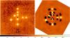 |
Fig. 1 Left: false colour image of fake planets injected at separation ranging from 0.27″ to 1.35″ in a cube with the same sky rotation as the science target. Right: residual image of these fake planets after weighted-ADI procedure were applied, simulating an on-sky rotation of 29°. Self-subtraction effects are visible as negatives “wings” around the fake planets. The rotation centre for the ADI procedure is marked by a black cross. A logarithmic scale is used. |
3.2.3. 2D detection limits maps
We took particular care to derive an accurate and meaningful detection limit map around each of our targets. The first step was to produce a noise map of each of our final residual image, by measuring the pixel noise within sliding square boxes of 5 × 5 pixels (typically ~ 1.5 × FWHM). This provides the noise per pixel and could be used directly to derive the peak value of a signal that would be above a given S/N threshold. However, since actual detections do not rely on a single pixel being above a S/N threshold, we preferred to derive the 5σ detection limit on a 1.5 × FWHM-diameter aperture, comparing the noise within the aperture to the flux of the unsaturated PSF of each target within the same aperture.
In the case of ADI-reductions, a second step was to correct these detection maps from the flux loss caused by self-subtraction. We created cubes of images of high-S/N fake planets with the same field rotation as the science images and applied the same ADI procedures as used for the science images. We compared the flux injected to the flux recovered by our detection pipeline on the final reduced fake planets images (see Fig. 1) to derive the actual flux loss due to self-subtraction in ADI-processing on a range of radius from the central star. Since these fake planet images are used to measure only self-subtraction effects, the central star is not included in the image. The effects of the central star residuals are already taken into account in the noise map produced in the previous step, where it dominates the local noise at short separations.
Finally, the detection limit in arbitrary detector unit was converted into a contrast in magnitudes by scaling it to the measured flux of the unsaturated science target. Figure 2 shows one instance of such a contrast map where the target is a close binary to illustrate the advantages of a 2D mapping approach over a 1D detection limit curve in a strongly asymmetrical case.
Such 2D contrast maps were produced for all targets and for all the reduction techniques used. Tables 3 and 4 give the median of the contrast achieved in each image both for a close separation area (<18.5 pixels = 0.5″) and a wider separation area (>18.5 pixels and < 100 pixels = 2.7″). Inner pixels for which there was not enough rotation to find a suitable PSF reference either in LOCI or sADI/wADI were removed from the statistics of all reduction modes. Computing values over a large area rather than over thin annuli and using the same pixels for each set of image, provides robust statistics to quantitatively compare different reduction techniques. These tables present detection limits obtained with a single set of ADI and LOCI parameters, and slightly better detection limits (typically by ≤ 0.3 mag ) can be obtained by manually fine tuning the parameters for each target, especially when using LOCI. We carried out such optimised analysis each time we had a hint that a potential candidate companion could be visible, but since the overall sensitivity gain was modest, we chose to present the more self-consistent detection limits obtained with a single set of parameters for all targets.
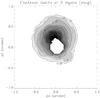 |
Fig. 2 Final contrast map for the GJ3305AB system. Contours identify magnitudes of contrast at 5σ achieved at a given position. The white area in the centre shows the position of the primary where no contrast was measurable and the dark zone slightly on the north is the higher noise area induced by GJ3305B. North is up and east left. |
Median contrast achieved at 5σ limit over a short ( ≤ 0.5″) separation area and a large separation area for targets observed with classical AO imaging (without ADI mode).
4. Results
4.1. Especially interesting targets
We describe a few specifically interesting objects case by case, notably two targets around which we identified candidate companions, none of which were physically associated with the central star.
4.1.1. 2M1139/TWA26
Our automatic detection routine identified a source 13σ above local background, at a separation ρ = 13.4″ and a position angle θ = 196° from 2M1139, at RA = 11:39:50.8 and Dec = −31:59:34.8.
A check of 2MASS images shows an H = 15.5 object at the position of our L′ detection. Since this object was also detected in USNO optical images, where it appears much brighter than the central star, it is obviously too blue and too bright to be a lower mass companion of 2M1139. This was further confirmed by its proper motion which is not compatible with the proper motion, of 2M1139, at more than 10σ.
4.1.2. The GJ3305 AB system
GJ3305B.
GJ3305 has been identified by Kasper et al. (2007) as a low-contrast close binary. Figure 4 shows the reduced image side-to-side with the residual map after simple ADI subtraction. GJ3305B appears clearly in both images at a PA of 19.2° and a separation of 0.27″. Its Airy rings are visible in the residual image up to the 6th, a telltale sign of the effectiveness of the primary subtraction. By combining archive data of GJ3305AB shown in Table 5 with our L′ observations we have seven independent astrometric measurements of GJ3305B. Since they are relatively regularly sampling a significant fraction of the full orbit, we attempted a Levenberg-Marquardt fit of an orbit for the system. We fixed the mass of this 12 Myr-old βPictoris moving group system to 0.85 + 0.5 = 1.35 M⊙ using stellar evolution models from Baraffe et al. (2003). Though we do not have enough astrometric points to derive accurate orbital parameters, the fit consistently converged towards solutions where the orbit is seen nearly edge-on (i ~ 93°), with low eccentricity (e ~ 0.05), a resulting period of 20–25 years, and a semi-major axis of 8–9 AU, see Fig. 3. Since only about one third of the orbital period is covered by observations, the uncertainties are high, and it is not currently possible to accurately constrain the mass of the system.
Position angle and separation of GJ3305B over the years.
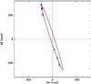 |
Fig. 3 Best fit for GJ3305B orbit projected on the sky in black, corresponding to a period of 21.5 yr, and eccentricity of 0.06, a semi-major axis of 8.5 AU, and an inclination of 93.2°. Observational astrometric points are in blue and the periastron is highlighted in green. |
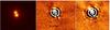 |
Fig. 4 Left: final stacked false-colour image of GJ3305AB from 2009 December data, in L′. North is up and east is to the left. Logarithmic scale is used. Centre: residual image of GJ3305AB from 2009 December data, after GJ3305A is subtracted by simple ADI. GJ3305B and the candidate companion are highlighted with green circles. Linear scale is used. Right: residual image of GJ3305AB from 2011 September data, after GJ3305A is subtracted by simple ADI. No source is detected at the 2009 position of the 2009 source. The position expected for this source in case it was a background object is highlighted by a green circle. Linear scale is used. North is up and east to the left. |
Candidate companion to GJ3305AB.
Another interesting source was identified around GJ3305AB in December 26, 2009 images, at a PA of 224 ± 2° and a radius of 0.38″ from GJ3305A. Since this source sits opposite to GJ3305B and between its Airy rings, it is located in a relatively clean area of the residual map, and the automatic detection routine identifies it as a 6 to 11σ detection in all the different residuals maps produced with the different ADI techniques. It was, however, located very close to the second Airy ring of the primary, and could be a speckle. Though it is likely this 2009 source was affected by speckle noise on the Airy ring, it was significantly above this local noise, and the presence of ADI negative signatures around it supported it as a real on-the-sky source rather than a speckle artefact.
The resulting contrast with the primary in L′ is around nine magnitudes, far too faint to be detected at similar separations in all but one of the earlier dataset of GJ3305, the 2004 December 15, NACO L′ data from which GJ3305B was initially identified. We retrieved the data from the ESO archive and reduced it. Unfortunately given the lower exposure time and the now superseded ADI techniques used for these observations, the noise at the position -assuming it is physically associated- of the faint candidate companion was higher than its expected signal and could not be used to confirm the detection. In the hypothesis that this object is a background source, the proper motion of GJ3305 is too low and not radial enough (RA = +46 mas yr-1 and Dec = − 65 mas yr-1) to bring the source out of the speckle-dominated area, where it would have been detectable. Since we also could not either rule out this hypothesis on the basis of archive data, further observations were necessary.
These observations were carried out with NACO at the VLT on September 1, 2011 and reduced following the ADI procedures described in Sect. 3. The exposure time, rotation, and the resulting detection limits for these new observations were slightly higher than those achieved on the 2009 data with which the candidate companion was identified. No source is detected in 2011 in the – small – area compatible with the orbital motion of a 11 AU planetary companion to GJ3305AB. This source is therefore not a planetary companion. A faint source is located close to the position expected if the 2009 detection was a background object. However, the flux measured on this source in 2011 is ~0.7 mag fainter than the flux of the 2009 candidate, raising doubt about the physical nature of both detections. As a consequence, these data cannot establish whether the 2009 candidate was a background object or a speckle noise bump, but they allow it to be excluded as a planetary companion. The residual images at both dates are shown in Fig. 4.
4.1.3. AU Mic/HIP102409
AU Mic. is known to harbour a edge-on debris disc (Song et al. 2002) which has been imaged using HST/ACS coronography down to 7.5 AU (Krist et al. 2005). Their HST images show no significant trace of gravitational perturbation of the disc by a large planetary body at close separation. We derived accurate detection probabilities as described in Sect. 4.2 and show that our data are able to exclude any presence of a planetary companion as light as 0.6 MJup beyond 20 AU with >90% confidence (see Fig. 5), and improves on the previous non-detections by Krist et al. (2005) and Kasper et al. (2007). Since our detection limits show some sensitivity down to Saturn mass objects, below the lowest masses available in the AMES-DUSTY model grid (0.5 MJup), we extrapolated values between 0.3 MJup and 0.5 MJup, resulting in higher uncertainties in this mass range.
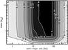 |
Fig. 5 Planetary detection probability around AU Mic. Numbers on the contours indicate the detection probability, taking the projection effects into account that could hid a planet in the line of sight of the central star on a fraction of its orbit. The semi-major axis values are therefore in real AU and not in projected AU. |
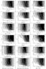 |
Fig. 6 Detection probability as a function of the mass and semi-major axis of the planets obtained with the MESS code (see text), for all the targets. |
4.2. Constraints on the existence of planetary mass companions
To evaluate the giant-planet detection probability around the targets in our survey, we used the MESS code (Bonavita et al. 2012). For each star, the code generates 103 orbits per grid point in a mass versus semi-major axis (SMA) grid with a sampling of 0.5 AU in SMA axis and 0.5 Mjup in mass. The orbits are randomly oriented in space, and the eccentricities were also randomly generated with a uniform distribution (with e < 0.6). For each random event, the code then evaluated the projected separation and the position of the planet on the projected orbit at the time of the observation. With this approach we could consider projection effects, and then constraint the actual semi-major axis of the planets, instead of the projected separation, while also using the whole spatial information coming from the 2D detection limit maps evaluated in Sect. 3.2.3. The mass limits are obtained by translating these flux detection limits into mass using the COND-base models (Allard et al. 2001; Baraffe et al. 2003) for temperatures below 1700 K and DUSTY-based models (Chabrier et al. 2000) for higher temperatures. The mass of the artificial planet is then compared to the detectable mass at that position on the detection map, and the fraction of orbits at each grid point that turn out to be detectable then correspond to the probability of detection at that grid point.
The resulting detection probability for each target are shown in Fig. 6. Figure 7 illustrates the mass-detection limits of the full survey, by averaging the 14 mass-detection probabilities maps of our targets with an accurate age measurment, and therefore excluding HIP114046 and 2M0443. The decreasing detection probability for a very large semi-major axis reflects the possibility that such objects can be observed within our 19.5 × 19.5″ field of view only on a fraction of their orbit and for a favourable combination of excentricity and angle of sight. Using the full 52-star sample, these limits could be used to derive constraints on the existence of giant planets around late-type stars and consequently on planetary formation models around low-mass stars. However, the sub-sample of 16 stars we present here is too small to derive meaningful statistics, so more observations are needed to bring it to a more statistically robust size.
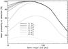 |
Fig. 7 Summary of the detection probabilities of the survey for a range of companion masses, obtained by averaging the detection probabilities of the 14 targets with an accurate age determination. The semi-major axis values are therefore in real AU, not projected AU. |
5. Conclusion
We presented the results of the deepest imaging survey of young M dwarfs to date, using L′ imaging with NACO at VLT. After developing a dedicated reduction and analysis pipeline, we achieved detections limits in average down to 1.5 MJup beyond 20 AU and up to 100–200 AU, and 3 MJup at 10 AU. On the closest and latest targets, we achieved detection limits well below the mass of Jupiter beyond 10 AU, therefore actually starting to probe (on 5 objects) the mass/separation range where planets around M dwarfs are supposed to be be more frequent (Gould et al. 2010; Bonfils et al. 2011), but found none. We also probed the high planetary mass range (M < 13 MJup) at close separations, reaching planetary sensitivity at 5 AU or less on nine out of our 16 targets. In spite of these deep observations, we found only one planetary companion, 2M1207B, discovered by Chauvin et al. (2004), in this sample of young M dwarfs. Unfortunately, our sample is currently too small to derive meaningful constraints on the existence of giant planets around late type stars, beyond the simple statement that giant planets more massive than 1 MJup are not common. With the same statistical limitations, our data also support the “brown dwarfs desert” hypothesis (Halbwachs et al. 2000) down to the lowest brown dwarf masses, since we find no brown dwarfs companions, while our survey had on average more than 95% de-projected sensitivity to brown dwarfs beyond 15 AU and could discover a fraction of them as close as 5 AU from the central star. Further deep observations in L′ of such targets are needed to increase our statistical significance and to put stronger constraints on formation models around low-mass stars.
Acknowledgments
We acknowledge financial support from the French Programme National de Planétologie (PNP, INSU) and from the French National Research Agency (ANR) through the GuEPARD project grant ANR10-BLANC0504-01. P.D. was financed by a grant from the Del Duca foundation. We thank David Lafrenière for his precious help with the LOCI code. This research has made use of the VizieR catalogue access tool, of the SIMBAD database, and of Aladin, operated at the CDS, Strasbourg. We thank the referee for her/his accurate comments.
References
- Agüeros, M. A., Covey, K. R., Lemonias, J. J., et al. 2011, ApJ, 740, 110 [NASA ADS] [CrossRef] [Google Scholar]
- Ahmic, M., Jayawardhana, R., Brandeker, A., et al. 2007, ApJ, 671, 2074 [NASA ADS] [CrossRef] [Google Scholar]
- Allard, F., & Freytag, B. 2010, Highlights of Astronomy, 15, 756 [Google Scholar]
- Allard, F., Hauschildt, P. H., Alexander, D. R., Tamanai, A., & Schweitzer, A. 2001, ApJ, 556, 357 [NASA ADS] [CrossRef] [Google Scholar]
- Baraffe, I., Chabrier, G., Barman, T. S., Allard, F., & Hauschildt, P. H. 2003, A&A, 402, 701 [NASA ADS] [CrossRef] [EDP Sciences] [Google Scholar]
- Barnes, S. A. 2003, ApJ, 586, 464 [NASA ADS] [CrossRef] [Google Scholar]
- Bate, M. R. 2009, MNRAS, 392, 590 [NASA ADS] [CrossRef] [Google Scholar]
- Bergfors, C., Brandner, W., Janson, M., et al. 2010, A&A, 520, A54 [NASA ADS] [CrossRef] [EDP Sciences] [Google Scholar]
- Biller, B., Allers, K., Liu, M., Close, L. M., & Dupuy, T. 2011, ApJ, 730, 39 [NASA ADS] [CrossRef] [Google Scholar]
- Boley, A. C. 2009, ApJ, 695, L53 [NASA ADS] [CrossRef] [Google Scholar]
- Bonavita, M., Chauvin, G., Desidera, S., et al. 2012, A&A, 537, A67 [NASA ADS] [CrossRef] [EDP Sciences] [Google Scholar]
- Bonfils, X., Delfosse, X., Udry, S., et al. 2011, A&A, submitted [Google Scholar]
- Boss, A. P. 2011, ApJ, 731, 74 [NASA ADS] [CrossRef] [Google Scholar]
- Bouy, H., Brandner, W., Martín, E. L., et al. 2003, AJ, 126, 1526 [NASA ADS] [CrossRef] [Google Scholar]
- Chabrier, G., Baraffe, I., Allard, F., & Hauschildt, P. 2000, ApJ, 542, 464 [NASA ADS] [CrossRef] [Google Scholar]
- Chauvin, G., Lagrange, A.-M., Dumas, C., et al. 2004, A&A, 425, L29 [NASA ADS] [CrossRef] [EDP Sciences] [MathSciNet] [Google Scholar]
- Cruz, K. L., Reid, I. N., Kirkpatrick, J. D., et al. 2007, AJ, 133, 439 [NASA ADS] [CrossRef] [Google Scholar]
- Currie, T., & Sicilia-Aguilar, A. 2011, ApJ, 732, 24 [NASA ADS] [CrossRef] [Google Scholar]
- Delorme, P., Collier Cameron, A., Hebb, L., et al. 2011, MNRAS, 413, 2218 [NASA ADS] [CrossRef] [Google Scholar]
- Dodson-Robinson, S. E., Veras, D., Ford, E. B., & Beichman, C. A. 2009, ApJ, 707, 79 [NASA ADS] [CrossRef] [Google Scholar]
- Ehrenreich, D., Lecavelier Des Etangs, A., & Delfosse, X. 2011, A&A, 529, A80 [NASA ADS] [CrossRef] [EDP Sciences] [Google Scholar]
- Forveille, T., Bonfils, X., Lo Curto, G., et al. 2011, A&A, 526, A141 [NASA ADS] [CrossRef] [EDP Sciences] [Google Scholar]
- Gould, A., Dong, S., Gaudi, B. S., et al. 2010, ApJ, 720, 1073 [NASA ADS] [CrossRef] [Google Scholar]
- Halbwachs, J. L., Arenou, F., Mayor, M., Udry, S., & Queloz, D. 2000, A&A, 355, 581 [NASA ADS] [Google Scholar]
- Johnson, H. M., & Wright, C. D. 1983, ApJS, 53, 643 [NASA ADS] [CrossRef] [Google Scholar]
- Kalas, P., Graham, J. R., Chiang, E., et al. 2008, Science, 322, 1345 [NASA ADS] [CrossRef] [PubMed] [Google Scholar]
- Kasper, M., Apai, D., Janson, M., & Brandner, W. 2007, A&A, 472, 321 [NASA ADS] [CrossRef] [EDP Sciences] [Google Scholar]
- Kennedy, G. M., & Kenyon, S. J. 2008, ApJ, 673, 502 [NASA ADS] [CrossRef] [Google Scholar]
- Kiss, L. L., Moór, A., Szalai, T., et al. 2011, MNRAS, 411, 117 [NASA ADS] [CrossRef] [Google Scholar]
- Kratter, K. M., Murray-Clay, R. A., & Youdin, A. N. 2010, ApJ, 710, 1375 [NASA ADS] [CrossRef] [Google Scholar]
- Krist, J. E., Ardila, D. R., Golimowski, D. A., et al. 2005, AJ, 129, 1008 [NASA ADS] [CrossRef] [Google Scholar]
- Lacy, C. H. 1977, ApJS, 34, 479 [NASA ADS] [CrossRef] [Google Scholar]
- Lafrenière, D., Marois, C., Doyon, R., Nadeau, D., & Artigau, É. 2007, ApJ, 660, 770 [NASA ADS] [CrossRef] [Google Scholar]
- Lagrange, A.-M., Bonnefoy, M., Chauvin, G., et al. 2010, Science, 329, 57 [NASA ADS] [CrossRef] [PubMed] [Google Scholar]
- Lépine, S., & Simon, M. 2009, AJ, 137, 3632 [NASA ADS] [CrossRef] [Google Scholar]
- Marois, C., Lafrenière, D., Doyon, R., Macintosh, B., & Nadeau, D. 2006, ApJ, 641, 556 [Google Scholar]
- Marois, C., Macintosh, B., Barman, T., et al. 2008, Science, 322, 1348 [NASA ADS] [CrossRef] [PubMed] [Google Scholar]
- Marois, C., Zuckerman, B., Konopacky, Q. M., Macintosh, B., & Barman, T. 2010, Nature, 468, 1080 [NASA ADS] [CrossRef] [PubMed] [Google Scholar]
- Mayor, M., & Queloz, D. 1995, Nature, 378, 355 [NASA ADS] [CrossRef] [Google Scholar]
- Nielsen, E. L., & Close, L. M. 2010, ApJ, 717, 878 [NASA ADS] [CrossRef] [Google Scholar]
- Nordström, B., Mayor, M., Andersen, J., et al. 2004, A&A, 418, 989 [NASA ADS] [CrossRef] [EDP Sciences] [Google Scholar]
- Pasinetti Fracassini, L. E., Pastori, L., Covino, S., & Pozzi, A. 2001, A&A, 367, 521 [NASA ADS] [CrossRef] [EDP Sciences] [Google Scholar]
- Perryman, M. A. C., Brown, A. G. A., Lebreton, Y., et al. 1998, A&A, 331, 81 [NASA ADS] [Google Scholar]
- Plavchan, P., Werner, M. W., Chen, C. H., et al. 2009, ApJ, 698, 1068 [NASA ADS] [CrossRef] [Google Scholar]
- Rafikov, R. R. 2011, ApJ, 727, 86 [NASA ADS] [CrossRef] [Google Scholar]
- Reiners, A., & Basri, G. 2009, ApJ, 705, 1416 [NASA ADS] [CrossRef] [Google Scholar]
- Scholz, A., Jayawardhana, R., & Wood, K. 2006, ApJ, 645, 1498 [NASA ADS] [CrossRef] [Google Scholar]
- Song, I., Weinberger, A. J., Becklin, E. E., Zuckerman, B., & Chen, C. 2002, AJ, 124, 514 [NASA ADS] [CrossRef] [Google Scholar]
- Stamatellos, D., Maury, A., Whitworth, A., & André, P. 2011, MNRAS, 413, 1787 [NASA ADS] [CrossRef] [Google Scholar]
- Torres, C. A. O., Quast, G. R., da Silva, L., et al. 2006, A&A, 460, 695 [NASA ADS] [CrossRef] [EDP Sciences] [Google Scholar]
- Torres, C. A. O., Quast, G. R., Melo, C. H. F., & Sterzik, M. F. 2008, in Young Nearby Loose Associations, ed. B. Reipurth, 757 [Google Scholar]
All Tables
Rotation periods and corresponding gyrochronological ages derived for HIP114046 assuming different values for the inclination angle i.
Median contrast achieved for ADI-compatible observations, ranked by field-rotation, at 5σ limit for short ( ≤ 0.5″) and large separation areas.
Median contrast achieved at 5σ limit over a short ( ≤ 0.5″) separation area and a large separation area for targets observed with classical AO imaging (without ADI mode).
All Figures
|
Fig. 1 Left: false colour image of fake planets injected at separation ranging from 0.27″ to 1.35″ in a cube with the same sky rotation as the science target. Right: residual image of these fake planets after weighted-ADI procedure were applied, simulating an on-sky rotation of 29°. Self-subtraction effects are visible as negatives “wings” around the fake planets. The rotation centre for the ADI procedure is marked by a black cross. A logarithmic scale is used. |
| In the text | |
|
Fig. 2 Final contrast map for the GJ3305AB system. Contours identify magnitudes of contrast at 5σ achieved at a given position. The white area in the centre shows the position of the primary where no contrast was measurable and the dark zone slightly on the north is the higher noise area induced by GJ3305B. North is up and east left. |
| In the text | |
|
Fig. 3 Best fit for GJ3305B orbit projected on the sky in black, corresponding to a period of 21.5 yr, and eccentricity of 0.06, a semi-major axis of 8.5 AU, and an inclination of 93.2°. Observational astrometric points are in blue and the periastron is highlighted in green. |
| In the text | |
|
Fig. 4 Left: final stacked false-colour image of GJ3305AB from 2009 December data, in L′. North is up and east is to the left. Logarithmic scale is used. Centre: residual image of GJ3305AB from 2009 December data, after GJ3305A is subtracted by simple ADI. GJ3305B and the candidate companion are highlighted with green circles. Linear scale is used. Right: residual image of GJ3305AB from 2011 September data, after GJ3305A is subtracted by simple ADI. No source is detected at the 2009 position of the 2009 source. The position expected for this source in case it was a background object is highlighted by a green circle. Linear scale is used. North is up and east to the left. |
| In the text | |
|
Fig. 5 Planetary detection probability around AU Mic. Numbers on the contours indicate the detection probability, taking the projection effects into account that could hid a planet in the line of sight of the central star on a fraction of its orbit. The semi-major axis values are therefore in real AU and not in projected AU. |
| In the text | |
|
Fig. 6 Detection probability as a function of the mass and semi-major axis of the planets obtained with the MESS code (see text), for all the targets. |
| In the text | |
|
Fig. 7 Summary of the detection probabilities of the survey for a range of companion masses, obtained by averaging the detection probabilities of the 14 targets with an accurate age determination. The semi-major axis values are therefore in real AU, not projected AU. |
| In the text | |
Current usage metrics show cumulative count of Article Views (full-text article views including HTML views, PDF and ePub downloads, according to the available data) and Abstracts Views on Vision4Press platform.
Data correspond to usage on the plateform after 2015. The current usage metrics is available 48-96 hours after online publication and is updated daily on week days.
Initial download of the metrics may take a while.