| Issue |
A&A
Volume 538, February 2012
|
|
|---|---|---|
| Article Number | A56 | |
| Number of page(s) | 8 | |
| Section | Astronomical instrumentation | |
| DOI | https://doi.org/10.1051/0004-6361/201118476 | |
| Published online | 01 February 2012 | |
Advances in the interpretation and analysis of lunar occultation light curves⋆
1
National Astronomical Research Institute of Thailand,
191 Siriphanich Bldg., Huay Kaew Rd., Suthep,
Muang,
Chiang Mai
50200,
Thailand
e-mail: andrea@narit.or.th
2
European Southern Observatory, Karl-Schwarzschild-Str. 2, 85748
Garching bei München,
Germany
Received:
18
November
2011
Accepted:
23
December
2011
Context. The introduction of fast 2D detectors and the use of very large telescopes have significantly advanced the sensitivity and accuracy of the lunar occultation technique. Recent routine observations at the ESO Very Large Telescope have yielded hundreds of events with results, especially in the area of binary stars, which are often beyond the capabilities of any other techniques.
Aims. With the increase in the quality and in the number of the events, subtle features in the light curve patterns have occasionally been detected which challenge the standard analytical definition of the lunar occultation phenomenon as diffraction from an infinite straight edge. We investigate the possible causes for the observed peculiarities.
Methods. We have evaluated the available statistics of distortions in occultation light curves observed at the ESO VLT, and compared it to data from other facilities. We have developed an alternative approach to model and interpret lunar occultation light curves, based on 2D diffraction integrals describing the light curves in the presence of an arbitrary lunar limb profile. We distinguish between large limb irregularities requiring the Fresnel diffraction formalism, and small irregularities described by Fraunhofer diffraction. We have used this to generate light curves representative of several limb geometries, and attempted to relate them to some of the peculiar data observed.
Results. We conclude that the majority of the observed peculiarities is due to limb irregularities, which can give origin both to anomalies in the amplitude of the diffraction fringes and to varying limb slopes. We investigate also other possible effects, such as detector response and atmospheric perturbations, finding them negligible. We have developed methods and procedures that for the first time allow us to analyze data affected by limb irregularities, with large ones bending the fringe pattern along the shape of the irregularity, and small ones creating fringe amplitude perturbations in comparison to the ideal fringe pattern.
Conclusions. The effects of a variable limb slope can be satisfactorily corrected. More complex limb irregularities could be fitted in principle with a grid search based on the standard analytical model, however this method is time consuming and does not lead to unique solutions. The incidence of the limb perturbations is relatively small, but its significance is increased with the use of very large telescopes due both to the footprint at the lunar limb and to the increased sensitivity. In general, we recommend to observe occultations using sub-pupils. This will be a necessary requirement with the next generation of extremely large telescopes.
Key words: techniques: high angular resolution / occultations / Moon
© ESO, 2012
1. Introduction
Lunar occultations (LO) were first suggested as a high angular resolution technique capable of measuring stellar angular diameters already one century ago. The geometrical optics approach suggested by MacMahon (1908) was shown to be incorrect by Eddington (1908) who pointed out the role played by diffraction. The computational and technical requirements involved were such that the first suggestion to use the amplitude of the diffraction fringes to measure angular diameters and the first record of a light curve were published only decades later (Williams 1939; Whitford 1939). At that time, the measurement of small amplitude changes at frequencies close to 1 kHz posed a challenge, and further observations remained scarce (Evans 1951; Evans et al. 1953). LO started to be widely employed both at optical and near-IR wavelengths only in the 1970s and quickly picked up pace. A catalogue by White & Feierman (1987) listed LO-derived angular diameters for 124 stars. The serendipitous discovery of close binary and multiple stars by LO was a less anticipated but equally prolific line of results. In particular, we note the series of over 6000 LO events recorded by Evans et al. (1986, and references therein).
The following decade saw a marked increase of results from high angular resolution measurements (cf. Richichi et al. 2005), but by then other techniques such as long-baseline interferometry had begun to be competitive. Indeed, although simple and efficient, LO suffer from the drawbacks of being fixed-time events of randomly selected sources and not being easily repeated. Nevertheless, the technique continued to progress, with important improvements in data analysis and technology. Richichi (1989) introduced a method for the maximum-likelihood recovery of the brightness profile of arbitrarily complex source geometries. Methods were introduced to deal with slow-varying scintillation (Richichi et al. 1992), and the use of fast read-out of sub-windows in near-IR array was started (Richichi et al. 1996). This latter approach, which greatly improves the sensitivity by eliminating much of the background noise and fluctuations present in data from aperture photometers, has now been systematically implemented at the ESO VLT, where Richichi et al. (2011, and references therein) have obtained several hundreds of light curves with unprecedented accuracy. Combining a limiting sensitivity close to K = 12.5 mag and an angular resolution close to one milliarcsecond (mas), LO at a very large telescope are arguably the most powerful high angular resolution technique available at present.
Throughout this century of developments and progress in the LO technique, one assumption has remained essentially unchanged: the lunar limb is assumed to be an infinite straight edge. However, the quality of the LO data that can be obtained today is challenging this assumption. In this paper, we review both qualitatively and quantitatively the peculiarities observed in some of the light curves from the large sample of data obtained at the VLT with ISAAC, presently the best telescope and instrument combination for LO work.
First, we introduce the mathematical representation of LO light curves, both by the classical analytical formulae for diffraction by a straight edge, and by the general wave optics formalism. We employ this latter to simulate realistic situations such as non-straight edges. Subsequently we focus our attention on two main issues: perturbations to the fringe amplitudes and changes in fringe frequency. We are able to explain, and partly correct, many of the observed peculiarities. We comment on the frequency with which these peculiarities can affect LO light curves and provide recommendations on how to minimize them.
2. Occultation light curves and limb irregularities
It is well known that the lunar surface is rugged and therefore the issue of the effects of lunar mountains was raised already in the early history of LO. The computations involved were significantly complex and simplifications had to be made. Diercks & Hunger (1952) found that, depending on the scale of the limb irregularities, in extreme cases the resulting occultation light curves could be significantly altered. Evans (1970) continued with more work under simple geometrical scenarios, and concluded that although the effects could be significant in principle, their incidence was in practice negligible as demonstrated by his extensive observational experience:“the whole problem might turn out to be of rather minor importance”.Using basic considerations on the scale and distribution of limb irregularities, Murdin (1971) arrived at similar conclusions. Since then, the issue has remained essentially untouched.
The geometry of an occultation is schematically represented in Fig. 1. The Moon moves over a background star with vector motion VM, and SD and SR mark the points of disappearance and reappearance. PA and CA are the position and contact angles, respectively. The lunar limb might have a local slope, denoted by the angle ψ. The effective rate of lunar motion will thus be VMcos(CA + ψ), and the source will be scanned along the angle PA + ψ.
The local slope describes the situation when a smooth mountain slope moves in the line of sight. Other structures as small as a few meters, e.g. large boulders, also affect the fringe pattern. In order to model arbitrary shapes of the lunar limb we adopt a semi-analytic formalism permitting to calculate the two-dimensional fringe pattern on the surface of the Earth as a function of the limb profile. Computing the fringe pattern on the ground generates a more easily interpreted graphic image of the problem than the discussion of individual light curves in the past.
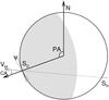 |
Fig. 1 Geometry of a lunar occultation and associated quantities. |
The analytical expression for the diffraction of the star light at the lunar limb is given
by Fresnel diffraction when the Moon is regarded as an infinite straight edge. The amplitude
V(x) of the light wave on the surface of
the Earth can be written as (Glindemann 2011)
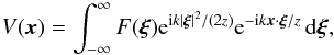 (1)omitting
a factor 1/(iλz). We denote by z the distance to the Moon
(≈ 3.8 × 10⁸ m), by F(ξ) the
limb profile as a function of the two-dimensional coordinate vector
ξ = (ξ,ζ) and by λ the
wavelength. Figure 2 displays an example for a limb
profile. In general, V(x) is a complex
function and we denote its phase by φ(x).
(1)omitting
a factor 1/(iλz). We denote by z the distance to the Moon
(≈ 3.8 × 10⁸ m), by F(ξ) the
limb profile as a function of the two-dimensional coordinate vector
ξ = (ξ,ζ) and by λ the
wavelength. Figure 2 displays an example for a limb
profile. In general, V(x) is a complex
function and we denote its phase by φ(x).
It is straightforward to compute the intensity of the diffraction pattern as a function of
the coordinate vector x on the ground as 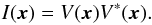 (2)Extensions
to the case of non-monochromatic and non-point like sources are possible by convolution
expressions that we do not pursue here.
(2)Extensions
to the case of non-monochromatic and non-point like sources are possible by convolution
expressions that we do not pursue here.
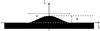 |
Fig. 2 The irregularity of the lunar limb as a simple structure proportional to 1+cos above the limb. The limb profile is given by the function F(ξ,ζ) that is zero in the black area and unity elsewhere. Two cases were investigated, one with w = 200 m and h = 25 m, the other with w = 12.5 m and h = 1.5 m. |
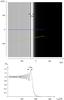 |
Fig. 3 2D diffraction pattern of a perfectly straight edge for
λ = 2.2 μm on the surface of the Earth
(top) as a function of the coordinate (x,y) on the
ground, and two light curves (bottom) scanned perpendicular to the
fringe pattern with local limb slopes of 0° (blue line) and of about 10° (yellow
line). The light curves display different fringe spacing depending on the angle of the
scan. Note that the diffraction pattern scales
with |

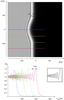 |
Fig. 4 Same as Fig. 3, for a large limb irregularity of about 25 × 200 m (see Fig. 2). The light curves (bottom) are scanned at different locations along the fringe pattern, coded by colours. For clarity, the light curves are shifted with respect to each other. The large irregularity disturbs the ideal pattern by bending it along its profile, modifying the measured fringe spacing as a function of local slope ψ. The inset displays an example of two selected light curves with different fringe spacing taken at y = 0 and at y = −50 m. The local slope ψ at y = −50 m (yellow line) affects the fringe spacing in the same way as the tilted scan in Fig. 3 (also in yellow). |
We simplify the description by replacing the function F(ξ) by Fe(ξ) + Fi(ξ), the sum of two functions: the straight edge and the irregularity. This is displayed in Fig. 2 where the straight edge fills the half-plane ζ < 0, and the irregularity, proportional to 1+cos, is placed on top, centered at ξ = 0. Naturally, this approach can be applied to any kind of irregularity. The diffraction integral in Eq. (1) can then be split into the sum of two integrals.
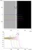 |
Fig. 5 Same as Fig. 4, for a smaller limb irregularity of about 1.5 × 12.5 m (see Fig. 2). An irregularity of this size and shape perturbs the ideal fringe pattern by adding a faint ring structure to it so that the light curves display different fringe amplitudes depending on the exact location of the scan. |
To compute the diffraction pattern of the irregularity
Fi(ξ), which is a small opaque
obstacle, we apply the Babinet principle (Born & Wolf 1970), stating that the diffraction pattern of this opaque obstacle is the same as
that of an infinite opaque screen with an opening shaped like
Fi(ξ). The only difference is
that the diffraction amplitude undergoes a phase shift of π. We consider
this by replacing Fi(ξ) by
−Fi(ξ) under the integral,
yielding 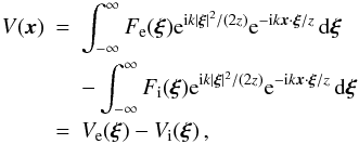 (3)when
we now think of Fi(ξ) as a small
opening with the shape of the irregularity in an otherwise opaque screen.
(3)when
we now think of Fi(ξ) as a small
opening with the shape of the irregularity in an otherwise opaque screen.
While the diffraction pattern of the straight edge is well known, producing fringes on the Earth with a spacing between the first maximum and the first minimum of about 13 m in the near infrared (see Fig. 3), the diffraction amplitude Vi(ξ) of an irregularity depends on its size and shape. Figures 4 and 5 show the effects on the diffraction patterns for different sizes of limb irregularities similar to that of Fig. 2. Different locations of the irregularity are represented by the colored horizontal lines. The motion of the Moon over the background star is equivalent to a telescope on the ground scanning the patterns, in our figures horizontally from left to right. Light curves are then recorded as a function of time, with typical rates of ≈ 0.5 m/ms. We remark that the slightly wiggly appearance of the curves in the figures is merely due to numerical approximations, and does not affect the conclusions.
2.1. Large and small irregularities
As long as the size ξ0 of the structure on the Moon is much
larger than  ,
i.e. much larger than 25 m in the near infrared, the Fresnel approximation, Eq. (3), has to be applied, and one finds that the
fringe pattern resembles more or less that of a straight edge bent along the shape of the
profile as displayed in Fig. 4.
,
i.e. much larger than 25 m in the near infrared, the Fresnel approximation, Eq. (3), has to be applied, and one finds that the
fringe pattern resembles more or less that of a straight edge bent along the shape of the
profile as displayed in Fig. 4.
However, if ξ0 is much smaller than
,
the quadratic phase term under the second integral in Eq. (3) can be neglected. Then the so-called Fresnel number
 /
is much smaller than unity and we move from Fresnel diffraction to Fraunhofer diffraction,
when a Fourier transform provides the diffraction amplitude
Vi(ξ). For a 25-m structure
the typical diffraction pattern displays very benign diffraction rings – akin to an Airy
disk – with a diameter of about 130 m. Compared to the diffraction pattern of the straight
edge with fringes spaced by 13 m, the diffraction pattern of the small structure varies
much slower in amplitude Vi(ξ)
and phase φi(x). We will see
below that these diffraction rings are irrelevant for the combined diffraction pattern.
/
is much smaller than unity and we move from Fresnel diffraction to Fraunhofer diffraction,
when a Fourier transform provides the diffraction amplitude
Vi(ξ). For a 25-m structure
the typical diffraction pattern displays very benign diffraction rings – akin to an Airy
disk – with a diameter of about 130 m. Compared to the diffraction pattern of the straight
edge with fringes spaced by 13 m, the diffraction pattern of the small structure varies
much slower in amplitude Vi(ξ)
and phase φi(x). We will see
below that these diffraction rings are irrelevant for the combined diffraction pattern.
Computing the product of the sum of the amplitudes and their complex conjugate as in
Eq. (2) we obtain the intensity of the
diffraction pattern of the lunar limb as  (4)composed
of the diffraction pattern of the straight edge
|Ve(x)|2, the
diffraction pattern of the irregularity
|Vi(x)|2 and
a mixed term. For a structure on the Moon that is much smaller than 25 m, i.e. for
NF ≪ 1, the diffraction pattern of the limb is governed by
that of the straight edge
|Ve(x)|2 and by the mixed
term, which adds a faint ring structure in form of half circles, as displayed in
Fig. 5. The spacing of these rings is the same as
the spacing of the fringes. The additional term
|Vi(x)|2,
which is the diffraction pattern of the irregularity alone, adds only negligible intensity
to the pattern. If the structure is further reduced in size the faint ring structure fades
away until it disappears. It should be stressed that the spacing between the rings is
independent of the size and form of the structure as long as it is much smaller
than .
(4)composed
of the diffraction pattern of the straight edge
|Ve(x)|2, the
diffraction pattern of the irregularity
|Vi(x)|2 and
a mixed term. For a structure on the Moon that is much smaller than 25 m, i.e. for
NF ≪ 1, the diffraction pattern of the limb is governed by
that of the straight edge
|Ve(x)|2 and by the mixed
term, which adds a faint ring structure in form of half circles, as displayed in
Fig. 5. The spacing of these rings is the same as
the spacing of the fringes. The additional term
|Vi(x)|2,
which is the diffraction pattern of the irregularity alone, adds only negligible intensity
to the pattern. If the structure is further reduced in size the faint ring structure fades
away until it disappears. It should be stressed that the spacing between the rings is
independent of the size and form of the structure as long as it is much smaller
than .
This effect is intuitively comprehensible since the small structure could be regarded as emitting spherical waves that, in combination with the diffraction at the edge, creates a ring structure in the intensity.
In Fig. 5, light curves of different scans through the diffraction pattern are displayed. Due to the overlap of the fringe pattern with the ring structure, the first maximum of the resulting fringe pattern increases with distance from the center. The second scan (yellow curve), about 25 m from the center shows a relative maximum. This corresponds to the first maximum of the ring structure adding intensity to the maximum of the fringe pattern. The influence of the irregularity disappears at about 40-50 m from the center when the additional ring structure becomes too faint. Note that for small irregularities the local slope ψ is not very helpful for the interpretation of the shape of the fringe pattern.
Moving to larger structures, the ring structure becomes more and more dominant, bending the whole fringe pattern eventually. One can no longer distinguish the influence of the three terms in Eq. (4). They combine in such a way, that the resulting fringe pattern is bent along the lunar limb as displayed in Fig. 4. Then there are only small increases of the first maximum, that we shall call overshoots, but their location and strength depend on the exact shape of the irregularity. However, in this case the variable fringe spacing is the more dominant effect which is well known and can be explained by the local slope ψ.
In conclusion, both varying fringe spacing and overshoot of the maxima of the fringe pattern can be explained by irregularities of the lunar limb. Very small structures tend to produce overshoots and larger structures cause varying fringe spacing due to fringe pattern that are bent along the profile of the irregularity. The influence of small irregularities disappears about 50 m from the center as already concluded by Diercks & Hunger (1952).
3. The nature and incidence of peculiarities in LO light curves
From the observations mentioned in Sect. 1, we have a database of over 2000 light curves. Most of them were obtained with a few combinations of different telescopes and instruments, and are therefore highly homogeneous. They have all been analyzed with the same suite of specifically designed software (Richichi et al. 1996). For our purposes we have selected two samples, with large and comparable numbers of observed events. On one side, we considered the TIRGO 1.5 m and the Calar Alto 1.2 m telescopes, each equipped with an InSb single pixel detector. We will denote this sample as TICA. On the other side, we considered the ESO VLT equipped with the ISAAC array detector operated in burst mode. In both cases mostly a broad band K filter was used, and occasionally other near-IR broad or narrow band filters. In particular at the VLT, sources with K ≲ 3.5 mag were observed with narrow-band filters to avoid saturation. The TICA set covers the years from 1985 to 2001. The instrumentation and the data have been reported in several papers, the most recent of which was Richichi & Roccatagliata (2005). The VLT data cover the period 2006 to current, with the most recent paper by Richichi et al. (2011). Many of the VLT data that we use for our statistics are not yet published. Table 1 reports the main statistics for the two sets under consideration. Two main kinds of anomalies have been observed, which we have already denoted as fringe overshoot and variable rate.
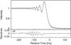 |
Fig. 6 Light curve (dots) for IRC−30355, and the best fit by a point source (solid line). The intensity has been normalized and time is counted from the moment of geometrical disappearance. The fringes show the overshoot effect discussed in the text. |
Statistics of two large LO samples.
3.1. Perturbations of fringe amplitude
Equation (1) prescribes that the diffraction fringes will have a maximum contrast for an unresolved source. This maximum contrast is defined by the details of the telescope, filter and integration time used, and can be computed quite accurately in the fitting process. This is a critical feature of LO, since it is precisely on the basis of the fringe contrast that angular diameters are measured. In a few cases however, it has been observed that actual fringes can have a higher contrast (hence our term overshoot) than the maximum theoretically possible. An example is provided in Fig. 6, for IRC−30355 reported by Richichi et al. (2011) as unresolved. It can be seen that the observed fringes exceed the contrast of the model light curve over most of the diffraction pattern, but not at the first fringe. In other cases, the overshoot has been seen to affect the first one or two fringes, but not the rest of the pattern. There is a marked correlation of this effect with the signal-to-noise ratio (SNR) of the light curve (and in turn, with the brightness of the source): it is present in 1.3% of the light curves with SNR < 50, and and in 6% of those with 50 < SNR < 500. This is consistent with a constant statistical distribution of limb irregularities, and with fringe amplitude distortions which are at most 2%, and more likely ≤1%, of the unocculted stellar signal.
3.2. Perturbations of fringe rate
The theory also predicts that, for a fixed apparent rate of motion of the limb as a straight edge, the fringe maxima and minima have a very precise position in time. Again, this is a critical feature since it represents a sort of internal clock allowing us to determine accurately the so-called limb slope. This can amount to several degrees, and ignoring it would lead to errors in the determination of the position angle and projected separation of binaries. Cases are present in our database, and have also been reported by other authors, in which the fringe positions cannot be fitted by a single value of the lunar rate of motion. Until now, no satisfactory fits could be performed for such data. One example is provided in Fig. 7, 2MASS 18015464-2529273 observed using the fast readout of a sub-window of an array detector (Richichi et al. 2011). The contact angle was −67°, leading to a slow rate of motion and covering a longer than usual section of the lunar limb. It can be noted that the rate changes appear to affect only a restricted portion around −300 ms, but light curves have been observed in which wider parts of the fringe pattern were affected. We note that the variable rate effect seems correlated with the contact angle. The median CA of the whole VLT sample is 28°, but the 21 events which exhibit this effect have a median CA of 65° (all angles modulo 90). This strengthens the view that the cause of this effects are slope changes along the lunar limb. By contrast, the overshoot effect is not correlated with the CA: the light curves exhibiting this effect have a median value of 31°, comparable to the whole sample.
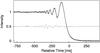 |
Fig. 7 A light curve with variable rate effects: 2MASS 18015464-2529273. The data (dots) have been normalized in intensity and time is counted from the moment of geometrical disappearance. The solid line is the best fit with the fixed-rate light curve of a point source. The dashed line shows the fit residuals, shifted by 0.5 units. More details in the text. |
3.3. Dependence on telescope size
As shown in Table 1, data obtained at the VLT are on average of higher SNR than the TICA ones. This is obvious when one considers the larger collecting area, and the reduction of the background afforded by pixel masking in array detectors. Another important, although less obvious, advantage is that a very large mirror will average out more turbulence cells, and therefore scintillation is greatly reduced. This is a limiting source of noise especially for bright stars.
It is then perhaps not surprising that a higher fraction of peculiarities are observed in the VLT data, considering that better SNR will lead to reveal smaller effects. Indeed, the probability of detecting possible fringe overshoots clearly increases with SNR, and the variable rate phenomenon will also depend on SNR at least when the smaller fringes are affected.
We also suggest another cause for the higher incidence of peculiarities in the VLT data, namely the fact that a larger telescope will be affected by irregularities from a longer section of the lunar limb. The ratio of the telescope diameters in the two cases is about 6, and the VLT diameter is smaller but yet comparable to what we have defined as a characteristic size of limb irregularities in Sect. 2. If this is the case, LO might present even more issues with telescopes in the 30–40 m class such as those planned for the generation of extremely large telescopes. The correct approach on telescopes of these sizes could be to divide the pupil in many areas and observe independently in each of them. This would provide the additional bonus of being able to observe simultaneously in different band-passes and to eliminate wavelength dependent sources of noise and perturbation. Suggestions to use sub-pupils were already presented e.g. by Takato (2003), and opto-mechanics with this capability is already encountered in modern instrumentation, e.g. in wavefront sensors for adaptive optics or in sparse aperture masking (Lacour et al. 2011).
4. Analysis of light curves with limb effects
Our knowledge of the lunar limb is still insufficient to be included as an a priori
information in the analysis LO light curves. Limb profiles are known from solar eclipses,
from ground-based and space imagery, and from grazing occultation events. The first two have
insufficient resolution: scales of  as obtained in the very best
ground-based images only address features above 200 m, significantly larger than those
affecting light curves as described in Sect. 2. A large
photographic survey which was converted into limb profiles by Watts (1963) also falls in this category: while very useful to improve the
accuracy of event prediction, it cannot reveal small changes of limb slopes. The dedicated
Clementine space mission provided some of the best maps of the Moon, but it was not complete
and had resolutions of 100 m at best on the lunar surface. Grazing occultations are indeed
valuable to map the lunar profile on scales of meters, however the limb coverage is mostly
confined to the polar regions and in any case largely incomplete (depending not only on the
lunar latitude but also on libration), with significant uncertainties on the exact location,
and not readily available. Thus, only a posteriori analysis of light curve irregularities is
possible in practice.
as obtained in the very best
ground-based images only address features above 200 m, significantly larger than those
affecting light curves as described in Sect. 2. A large
photographic survey which was converted into limb profiles by Watts (1963) also falls in this category: while very useful to improve the
accuracy of event prediction, it cannot reveal small changes of limb slopes. The dedicated
Clementine space mission provided some of the best maps of the Moon, but it was not complete
and had resolutions of 100 m at best on the lunar surface. Grazing occultations are indeed
valuable to map the lunar profile on scales of meters, however the limb coverage is mostly
confined to the polar regions and in any case largely incomplete (depending not only on the
lunar latitude but also on libration), with significant uncertainties on the exact location,
and not readily available. Thus, only a posteriori analysis of light curve irregularities is
possible in practice.
4.1. Limb distortions
From the arguments given in Sect. 2 and illustrated in Figs. 4 and 5, we conclude that an irregularly shaped lunar limb profile can give rise under specific circumstances to the fringe overshoot that is occasionally observed in real data. For example, we show in Fig. 8 a comparison between the light curves for an ideal straight limb and one similar to that of Fig. 2, about 80 m wide and 10 m high. The effect is remarkably similar to the overshoot illustrated in Fig. 6.
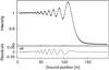 |
Fig. 8 Light curve for a monochromatic point source and an ideal straight lunar limb (solid line). The dots are the light curve for an arbitrary irregular limb. Note the similarity with Fig. 6. |
Unfortunately, while we can give an explanation for the effect, we are not able to provide a general method to retrieve the originating limb irregularities, apart from a time consuming trial-and-error process. In fact, there is no univocal correspondence and similar overshoot effects could be produced by different limb profiles.
Limb irregularities can give rise to decreased fringe amplitudes, i.e. undershoots, as well. During data analysis, however, only prominent increased amplitudes of the first fringe will stand out as non-physical as mentioned in Sect. 3.1, and this led us to concentrate on overshoots. The possible perturbation of fringe amplitudes in general can in principle bias the derivation of stellar diameters. In our experience, however, the overshoot or in general any fringe amplitude perturbation affects only a part of the train of fringes: sometimes the first fringe only is affected, other times only higher order fringes are perturbed. On the contrary, in the case of a resolved stellar disc, all fringe amplitudes are decreased consistently according to precise ratios. Therefore, it is in principle possible to safely discriminate between the effects of limb irregularities and of resolved stellar diameters.
4.2. Variable limb slope
A simplified case of limb irregularities is that of a variable limb slope. We have
assumed that the limb can indeed be well approximated by a straight edge, with a slope
ψ as mentioned in Sect. 2. Its
effect can be visualized as our telescope scanning through the patterns of Figs. 4 and 5 at an angle
ψ from the horizontal direction. We now consider that the slope varies
along the limb position. Therefore, as the star scans the lunar limb, our telescope scans
the diffraction pattern along a curved line, and the lunar rate
VL varies according to
 (5) We
approach this problem by letting the slope vary over n steps in a range
[ψ1,ψ2] ,
and by dividing the light curve into m sections. We have modified our
light curve fitting program, in order to generate a grid of
n × m models and to select at each light curve section
the slope which provides the best fit in the χ2 sense. This
requires of course also the generation of a proper noise model, which we construct as
described by Richichi et al. (1996).
(5) We
approach this problem by letting the slope vary over n steps in a range
[ψ1,ψ2] ,
and by dividing the light curve into m sections. We have modified our
light curve fitting program, in order to generate a grid of
n × m models and to select at each light curve section
the slope which provides the best fit in the χ2 sense. This
requires of course also the generation of a proper noise model, which we construct as
described by Richichi et al. (1996).
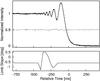 |
Fig. 9 The same light curve as shown in Fig. 7, now fitted with a variable limb slope as described in the text. Bottom: plot of the local limb slope as a function of time. |
The result of this approach is shown in Fig. 9 for the case of 2MASS 18015464-2529273 previously considered in Sect. 3. The top panel shows the composite fit, which is now quite satisfactory with the normalized χ2 improving from 3.2 (Fig. 7) to 1.4. The bottom part of Fig. 9 shows the recovered ψ(t) function. We experimented with various combinations of n,m and their range of variations, finding little dependence of χ2. The specific fit shown here was obtained letting VL vary by ±5% in 10 steps, and dividing the whole light curve in 40 sections where however only the sections between t = [−400,−200] ms were used for the fit, i.e. only 7 sections.
It can be seen that changes of ≈2° over 200 ms, or just under 50 m at the lunar limb, are sufficient to explain the observed peculiarities in the light curve considered here. In our experience with other light curves affected by similar problems, changes of up to 10° were observed. So far we have considered only the case of point like sources, but the method can be extended also to resolved sources without significant bias of the results since the resolved nature of a source is reflected mainly in the amplitude of the fringes and not in their position. We have also applied successfully this novel approach in the analysis of close binaries affected by variable limb slopes.
4.3. Other factors
We have considered also additional factors that could potentially cause small
perturbations of the measured fringe patterns. Atmospheric turbulence generates speckles
in images taken at high spatial and temporal resolution. For our conditions at the VLT, we
expect speckles with a characteristic angular size of about
 and temporal time scales of
about 50 ms, depending on atmospheric conditions. Our occultation frames recorded with
ISAAC have a pixel size of
and temporal time scales of
about 50 ms, depending on atmospheric conditions. Our occultation frames recorded with
ISAAC have a pixel size of  , and integration times of
3.2 ms. Therefore we expect some spatial averaging of speckles, and persistence over
several frames. To test this effect, sequences of simulated consecutive images of a point
source were generated (courtesy of M. Le Louarn) under realistic Paranal atmospheric
parameters, in noiseless conditions. The sequences consisted of many seconds of stellar
signal with the same pixel size, subarray dimensions and integration time as our data. We
applied the same masking procedure and examined different sections of 0.5 s duration, as
in our LO analysis. We found that speckle noise is about 50 times lower than the best
conditions in our observations (and possibly even lower due to numerical noise in the
simulations), and thus negligible in our data.
, and integration times of
3.2 ms. Therefore we expect some spatial averaging of speckles, and persistence over
several frames. To test this effect, sequences of simulated consecutive images of a point
source were generated (courtesy of M. Le Louarn) under realistic Paranal atmospheric
parameters, in noiseless conditions. The sequences consisted of many seconds of stellar
signal with the same pixel size, subarray dimensions and integration time as our data. We
applied the same masking procedure and examined different sections of 0.5 s duration, as
in our LO analysis. We found that speckle noise is about 50 times lower than the best
conditions in our observations (and possibly even lower due to numerical noise in the
simulations), and thus negligible in our data.
Another potential factor is the detector response, e.g. flat-fielding. Standard flat-field data, i.e. in full format and with long integration times, show fluctuations over a 32 × 32 array that are largely inferior to the typical read-out and photon noise. However, detectors such as the one used in ISAAC are not specified by the manufacturer and not characterized for the fast subarray mode that we employ. We have analyzed seven sequences of frames taken on the sky near the Moon, with the same burst mode and under the same conditions as our occultations. We have extracted from each 3 sections of 0.5 s as mentioned above, using a typical extraction mask. A light curve is affected by fringe overshoot if several points have intensity consistently deviating in excess of the model prediction for a point-source. Therefore, considering the typical fringe widths, and also that atmospheric coherence times at K are typically 50 ms or slower, we have rebinned our sequences to 22.4 ms (7 frames). We have then computed relative changes between pairs of consecutive, rebinned frames. The result is that, over the whole sample of sequences, the relative changes never exceed 1:3000 (average 1:7000). This is one order of magnitude more accurate than our best cases, and we are thus satisfied that the detector response in burst mode is not a major cause of the observed light curve peculiarities.
Finally, we have considered the potential effect of the slightly curved lunar limb, as opposed to the standard perfectly straight limb (Eq. (1)). Richichi (1990) provided a semi-analytical investigation over small angular sizes and found that in geometrical terms the difference between a straight and a curved limb cannot be detected for SNR ≲ 5 × 10³. In order to assess precisely the effect with our wave optics formalism, a numerical accuracy far superior to what we had readily available would be required. However, a quick comparison of the radius of curvature of the lunar limb (≈900″, or about 1.74 × 10⁶ m) with the structure of Fig. 2 is sufficient to convince us that any effect of the curved lunar limb would be orders of magnitude less than the perturbations shown in Figs. 4 and 5, and in practice negligible.
5. Conclusions
Lunar occultations (LO) observations at a very large telescope, such as the recent campaigns at the VLT with ISAAC (Richichi 2011, and references therein) have demonstrated a sensitivity of K ≈ 12 mag. In turn, SNRs for bright sources are routinely above 100, with values close to 500 in the best cases and showing the potential to reach 103 with more modern detectors.
Such high quality light curves are sometimes affected by small perturbations with respect to the expected models, which point to deviations of the lunar limb from the hypothesis of a straight infinite edge. Investigations of lunar limb effects were carried out by several authors already many decades ago, who found that perturbations of the light curves were possible and could be significant in special configurations, albeit generally unlikely as confirmed also by the then available observations. Such investigations, however, were significantly hampered by the numerical complexity of the equations and simplifications had to be introduced.
We have now taken advantage of the computational power easily available at present, to compute directly the light curves for any desired shape of the lunar limb from the general wave optics equations. We confirm earlier qualitative conclusions (e.g. Diercks & Hunger 1952) on the scale and influence of limb irregularities. In particular, we find that small structures (scales ≲25 m) are mainly responsible for changes in the fringe amplitudes, while structures ≳100 m are mainly affecting the fringe frequency. We have inspected and compared two large samples of homogeneous LO data, obtained at small and very large telescopes. We find that the frequency of anomalies in the light curves is higher for the latter, an occurrence that we explain on the basis of the higher average SNR as well as of the larger telescope footprint on the lunar limb. At extremely large telescopes, the ultimate performance of the method could be significantly hampered unless ad hoc observing solutions are adopted, such as the use of independent sub-pupils and their a posteriori recombination.
Most of the observed anomalies can be classified either as a fringe overshoot or as variable limb slope. Both can be reproduced by our formalism, however we are able to suggest a method to deal systematically only with the latter. In this case, the limb profile can be reliably estimated. In the case of the fringe overshoot we do not have a general solution for the limb profile. Concerning the fringe amplitudes, in principle a grid search can yield a profile which will be consistent with the observed perturbations, however the solution is not necessarily unique. A knowledge of the limb profile on the scale of ten meters would be required, which is at present not possible. Fringe amplitudes can be perturbed also in the opposite direction, i.e. decreased instead of increased. However, considering the required coherent decrease on all fringes, we conclude that this effect does not lead to fictitiously resolved angular diameters.
Acknowledgments
We thank M. Le Louarn for generating the simulated sequences of stellar images.
References
- Born, M., & Wolf, E. 1970, Principles of Optics (Oxford: Pergamon Press) [Google Scholar]
- Diercks, H., & Hunger, K. 1952, ZAp, 31, 182 [NASA ADS] [Google Scholar]
- Eddington, S. A. 1908, MNRAS, 69, 178 [NASA ADS] [Google Scholar]
- Evans, D. S. 1951, MNRAS, 111, 64 [NASA ADS] [Google Scholar]
- Evans, D. S. 1970, MNRAS, 75, 589 [NASA ADS] [Google Scholar]
- Evans, D. S., Heydenrych, C. R., & van Wyk, V. N. 1953, MNRAS, 113, 781 [NASA ADS] [Google Scholar]
- Evans, D. S., Edwards, D. A., Frueh, M., McWilliam, A., & Sandmann, W. H. 1985, AJ, 90, 2360 [NASA ADS] [CrossRef] [Google Scholar]
- Evans, D. S., McWilliam, A., Sandmann, W. H., & Frueh, M. 1986, AJ, 92, 1210 [NASA ADS] [CrossRef] [Google Scholar]
- Glindemann, A. 2011, Principles of Stellar Interferometry (Berlin Heidelberg: Springer-Verlag) [Google Scholar]
- Lacour, S., Tuthill, P., Amico, P., et al. 2011, A&A, 532, A72 [NASA ADS] [CrossRef] [EDP Sciences] [Google Scholar]
- MacMahon, P. A. 1908, MNRAS, 69, 126 [Google Scholar]
- Murdin, P. 1971, ApJ, 169, 615 [NASA ADS] [CrossRef] [Google Scholar]
- Richichi, A. 1989, A&A, 226, 366 [NASA ADS] [Google Scholar]
- Richichi, A. 1990, Ph.D. Thesis, University of Florence [Google Scholar]
- Richichi, A., & Roccatagliata, V. 2005, A&A, 433, 305 [NASA ADS] [CrossRef] [EDP Sciences] [Google Scholar]
- Richichi, A., Di Giacomo, A., Lisi, F., & Calamai, G. 1992, A&A, 265, 535 [NASA ADS] [Google Scholar]
- Richichi, A., Baffa, C., Calamai, G., & Lisi, F. 1996, AJ, 112, 278 [NASA ADS] [CrossRef] [Google Scholar]
- Richichi, A., Percheron, I., & Khristoforova, M. 2005, A&A, 431, 773 [NASA ADS] [CrossRef] [EDP Sciences] [Google Scholar]
- Richichi, A., Chen, W. P., Fors, O., & Wang, P. F. 2011, A&A, 532, A101 [NASA ADS] [CrossRef] [EDP Sciences] [Google Scholar]
- Takato, N. 2003, SPIE, 4841, 622 [NASA ADS] [CrossRef] [Google Scholar]
- Watts, C. B. 1963, Astron. Papers Amer. Ephem., 17, 1 [Google Scholar]
- White, N. M., & Feierman, B. H. 1987, AJ, 94, 751 [NASA ADS] [CrossRef] [Google Scholar]
- Whitford, A. E. 1939, ApJ, 89, 472 [NASA ADS] [CrossRef] [Google Scholar]
- Williams, J. D. 1939, ApJ, 89, 467 [NASA ADS] [CrossRef] [Google Scholar]
All Tables
All Figures
|
Fig. 1 Geometry of a lunar occultation and associated quantities. |
| In the text | |
|
Fig. 2 The irregularity of the lunar limb as a simple structure proportional to 1+cos above the limb. The limb profile is given by the function F(ξ,ζ) that is zero in the black area and unity elsewhere. Two cases were investigated, one with w = 200 m and h = 25 m, the other with w = 12.5 m and h = 1.5 m. |
| In the text | |
|
Fig. 3 2D diffraction pattern of a perfectly straight edge for
λ = 2.2 μm on the surface of the Earth
(top) as a function of the coordinate (x,y) on the
ground, and two light curves (bottom) scanned perpendicular to the
fringe pattern with local limb slopes of 0° (blue line) and of about 10° (yellow
line). The light curves display different fringe spacing depending on the angle of the
scan. Note that the diffraction pattern scales
with |
| In the text | |
|
Fig. 4 Same as Fig. 3, for a large limb irregularity of about 25 × 200 m (see Fig. 2). The light curves (bottom) are scanned at different locations along the fringe pattern, coded by colours. For clarity, the light curves are shifted with respect to each other. The large irregularity disturbs the ideal pattern by bending it along its profile, modifying the measured fringe spacing as a function of local slope ψ. The inset displays an example of two selected light curves with different fringe spacing taken at y = 0 and at y = −50 m. The local slope ψ at y = −50 m (yellow line) affects the fringe spacing in the same way as the tilted scan in Fig. 3 (also in yellow). |
| In the text | |
|
Fig. 5 Same as Fig. 4, for a smaller limb irregularity of about 1.5 × 12.5 m (see Fig. 2). An irregularity of this size and shape perturbs the ideal fringe pattern by adding a faint ring structure to it so that the light curves display different fringe amplitudes depending on the exact location of the scan. |
| In the text | |
|
Fig. 6 Light curve (dots) for IRC−30355, and the best fit by a point source (solid line). The intensity has been normalized and time is counted from the moment of geometrical disappearance. The fringes show the overshoot effect discussed in the text. |
| In the text | |
|
Fig. 7 A light curve with variable rate effects: 2MASS 18015464-2529273. The data (dots) have been normalized in intensity and time is counted from the moment of geometrical disappearance. The solid line is the best fit with the fixed-rate light curve of a point source. The dashed line shows the fit residuals, shifted by 0.5 units. More details in the text. |
| In the text | |
|
Fig. 8 Light curve for a monochromatic point source and an ideal straight lunar limb (solid line). The dots are the light curve for an arbitrary irregular limb. Note the similarity with Fig. 6. |
| In the text | |
|
Fig. 9 The same light curve as shown in Fig. 7, now fitted with a variable limb slope as described in the text. Bottom: plot of the local limb slope as a function of time. |
| In the text | |
Current usage metrics show cumulative count of Article Views (full-text article views including HTML views, PDF and ePub downloads, according to the available data) and Abstracts Views on Vision4Press platform.
Data correspond to usage on the plateform after 2015. The current usage metrics is available 48-96 hours after online publication and is updated daily on week days.
Initial download of the metrics may take a while.