| Issue |
A&A
Volume 538, February 2012
|
|
|---|---|---|
| Article Number | A13 | |
| Number of page(s) | 11 | |
| Section | Stellar atmospheres | |
| DOI | https://doi.org/10.1051/0004-6361/201118210 | |
| Published online | 26 January 2012 | |
VLT/X-shooter observations and the chemical composition of cool white dwarfs⋆,⋆⋆
Astronomický ústav, Akademie věd České republiky, Fričova 298,
25165
Ondřejov
Czech Republic
e-mail: kawka@sunstel.asu.cas.cz; vennes@sunstel.asu.cas.cz
Received: 5 October 2011
Accepted: 14 November 2011
We present a model atmosphere analysis of cool hydrogen-rich white dwarfs observed at the Very Large Telescope (VLT) with the X-shooter spectrograph. The intermediate-dispersion and high signal-to-noise ratio of the spectra allowed us to conduct a detailed analysis of hydrogen and heavy element line profiles. In particular, we tested various prescriptions for hydrogen Balmer line broadening parameters and determined the effective temperature and surface gravity of each star. The spectra of three objects (NLTT 1675, 6390, and 11393) show heavy elements (Mg, Al, Ca, or Fe). Our abundance analysis revealed a relatively high iron-to-calcium ratio in NLTT 1675 and NLTT 6390. We also present an analysis of spectropolarimetric data obtained at the VLT using the focal reducer and low dispersion spectrograph (FORS). We establish strict upper limits to the magnetic field strengths in three of the DAZ white dwarfs and determine the longitudinal magnetic field strength in the DAZ NLTT 10480. The class of DAZ white dwarfs comprises objects that are possibly accreting material from their immediate circumstellar environment and the present study helps to establish the class properties.
Key words: white dwarfs / stars: atmospheres / stars: abundances / stars: magnetic field
Based on observations collected at the European Organisation for Astronomical Research in the Southern Hemisphere, Chile under programme ID 080.D-0521, 082.D-0750, 083.D-0540, 084.D-0862 and 086.D-0562.
Appendices are available in electronic form at http://www.aanda.org
© ESO, 2012
1. Introduction
The first studies of heavy elements in cool hydrogen-rich (DA) white dwarfs were restricted to a few cases, i.e., the cool white dwarf G74-7 (Lacombe et al. 1983) and the ZZ Ceti star G29-38 (Koester et al. 1997) because of the rarity of these stars. Diffusion timescales in cool DA white dwarfs are relatively short (Paquette et al. 1986), and heavy elements were not expected to be detectable in the photosphere of these objects. Therefore, heavy elements such as calcium in G74-7 must be continuously supplied from an external source. Incidentally, Zuckerman & Becklin (1987) reported an infrared excess in G29-38, and Graham et al. (1990) showed that the excess is caused by the presence of circumstellar dust. The detection of heavy elements (Mg, Ca, Fe) in the atmosphere of G29-38 by Koester et al. (1997) strengthened the link between atmospheric contaminants and the presence of circumstellar material.
Surveys of white dwarfs conducted using high-dispersion spectrographs mounted on large aperture telescopes (e.g., Zuckerman et al. 1998, 2003; Koester et al. 2005) have shown that in contrast to earlier assessments, a significant fraction of DA white dwarfs, labeled DAZ white dwarfs, are contaminated with elements heavier than helium. Within a sample of ~100 DA white dwarfs that are not in close binary systems, Zuckerman et al. (2003) showed that ≈25% of the stars exhibit photospheric heavy element lines. For the majority of stars in their sample, only calcium lines are observed, but in some cases other elements such as magnesium, iron, aluminium, and silicon are also detected.
Our study of cool white dwarfs in the revised NLTT catalogue (Salim & Gould 2003) unveiled new cases of external contaminations. The stars were selected using a reduced proper motion diagram combined with optical and infrared colours (Kawka et al. 2004) resulting in a catalogue of ≈400 objects, only about half of which had previously been spectroscopically confirmed as white dwarfs. Although the NLTT catalogue is deemed incomplete at low Galactic latitude and far south (see Lépine & Shara 2005), it still contains many stars that remain largely unstudied. More complete catalogues utilizing the Digital Sky Surveys, such as the LSPM catalogue of stars with proper motions greater than 0.15′′ yr-1 (Lépine & Shara 2005) have been compiled and complement the NLTT catalogue where it is incomplete.
Kawka & Vennes (2006) conducted low-dispersion spectroscopic observations of white dwarf candidates from the NLTT catalogue and listed 49 new objects including 30 DA white dwarfs, three DAZ white dwarfs including NLTT 43806, and 16 non-DA white dwarfs. In follow-up observations of NLTT 43806, Zuckerman et al. (2011) obtained high signal-to-noise ratio (S/N) and high-dispersion spectra showing it to harbour a weak magnetic field.
In this work, we present intermediate-dispersion and high S/N spectroscopy and a model atmosphere analysis of new DAZ white dwarfs that were selected from the New Luyten Two-Tenths (NLTT) catalogue. These new objects complement the few hydrogen-rich white dwarfs that have been scrutinized for heavy elements other than calcium. We presented a first report of this programme with the analysis of the coolest DAZ in our sample (NLTT 10480; Kawka & Vennes 2011). The X-shooter spectrum of NLTT 10480 showed Zeeman-split calcium and hydrogen lines that revealed a surface magnetic field of Bs = 0.519 ± 0.004 MG. At the present time, only three other magnetic DAZ white dwarfs are known: G77-50 (Farihi et al. 2011), NLTT 43806 (Zuckerman et al. 2011), and LTT 8381 (Koester et al. 2009). Apart from these four magnetic DAZ white dwarfs, two more white dwarfs with helium-dominated atmospheres that are contaminated with heavy elements have also been shown to be weakly magnetic: G165-7 (Dufour et al. 2006) and LHS 2534 (Reid et al. 2001). Potter & Tout (2010) and Nordhaus et al. (2011) proposed that magnetic fields in white dwarfs may be generated during the common-envelope phase of interacting binaries. Applying this model to the case of G77-50, Farihi et al. (2011) proposed that the presence of a weak field in this star may be the result of a past common-envelope episode with a planetary component during the white dwarf’s formative years.
In Sect. 2, we describe our observations obtained at the European Southern Observatories (ESO) using the New Technology Telescope (3.6-m) and the Very Large Telescopes (VLTs) as well as the 4-m telescope at Cerro Tololo Inter-American Observatory (CTIO). Section 3 presents our model atmosphere analysis including details of the model structure (Sect. 3.1) and heavy-element line profile (Sect. 3.2) calculations. Using these models, we determine the effective temperature and surface gravity for each star (Sect. 3.3), and measure their heavy element abundance (Sect. 3.4). The stellar radial velocities and kinematics, and estimates of the magnetic field strengths are presented in Sects. 3.5 and 3.6, respectively. We summarize and discuss some implications of our results in Sect. 4.
2. Observations
2.1. Spectroscopy
Log of spectroscopic observations.
We first observed objects from the present sample during a programme aimed at identifying new white dwarfs in the NLTT catalogue. NLTT 6390 and NLTT 11393 were observed with the focal reducer and low dispersion spectrograph (FORS1) attached to the 8 m UT2 (Kueyen) at Paranal Observatory on UT 2007 November 1 and 3 as part of our spectropolarimetric survey of white dwarfs. The purpose of these observations was to confirm the nature of the observed sample of stars and to search for weak magnetic fields. We used the 600B grism combined with a slit-width of 1 arcsec that provided a resolution of 6 Å and a spectral range from 3780 Å to 6180 Å. The observations consisted of a sequence of two consecutive exposures. In the first exposure, the Wollaston prism was rotated to −45° followed by a second exposure where the Wollaston prism was rotated to +45°, from which we extracted the flux and circular polarization spectra.
As part of our identification programme, we observed NLTT 23966 with the R-C spectrograph attached to the 4 m telescope at CTIO on UT 2008 February 25. We used the KPGL2 (316 lines per mm) grating with the WG360 filter to block out the second order contamination. We set the slit-width to 1.5 arcsec, which provided a spectral resolution of ~8 Å and a spectral range of 3820 to 7500 Å. The spectra were flux calibrated with the flux standard GD 108. We also selected a sample of spectroscopically confirmed hydrogen-rich white dwarfs from the NLTT catalogue, including NLTT 23966, for spectropolarimetric observations with the aim of searching for weak magnetic fields. The white dwarf NLTT 23966 was observed with the FORS2 attached to the 8 m UT1 (Antu) at Paranal Observatory on UT 2010 Jan. 23. We used the 1200R grism with the order blocking filter GG435 and 2k × 4k MIT CCD. The slit-width was set to 1 arcsec which resulted in a spectral resolution of ~3 Å and a spectral range from 5810 Å to 7290 Å. The observations were carried out in the same way as for NLTT 6390 and NLTT 11393 with the FORS1 spectrograph, with one sequence consisting of two consecutive exposures with the Wollaston prism rotated 90° between the two exposures. Two sequences were obtained for NLTT 23966.
The white dwarf NLTT 1675 was first observed with the ESO Faint Object Spectrograph and Camera (EFOSC2) attached to the 3.6 m New Technology Telescope (NTT) at La Silla Observatory on UT 2009 August 24. We used grism 11, which has 300 lines per mm and a blaze wavelength of 4000 Å. The slit-width was set to 1 arcsec, which resulted in a spectral resolution of ~14 Å and a spectral range from 3700 Å to 7250 Å. We also observed NLTT 11393 using this setup on UT 2008 October 21. The observations were carried out at the parallactic angle and flux calibrated with the flux standard Feige 110.
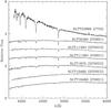 |
Fig. 1 Identification spectra, fλ versus λ, normalized at λ = 5500 Å and shifted up for clarity. |
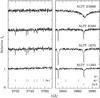 |
Fig. 2 X-shooter spectra covering iron (left) and calcium (right) lines in four cool, hydrogen-rich white dwarfs from the NLTT catalogue. Photospheric calcium lines are observed in three stars, while iron was only observed in NLTT 1675 and 6390. In contrast to our initial report (Kawka et al. 2011), our new X-shooter spectra show that NLTT 23966 is devoid of calcium. The possible identification of aluminium is reported for NLTT 1675. |
Line identifications.
Figure 1 shows the low-dispersion identification spectra of the five cool hydrogen-rich white dwarfs for which higher dispersion spectra were obtained with VLT/X-shooter, including the identification spectra of the cool magnetic DAZ NLTT 10480 that was analyzed by Kawka & Vennes (2011). The low dispersion spectra of these stars showed the Ca iiλ3933 Å line and were therefore selected for follow-up high-dispersion observations with X-shooter. In the case of NLTT 23966, the Ca iiλ3933 Å line seen in the CTIO spectrum was the result of background noise.
Following-up on our low-dispersion spectroscopic observations, we obtained a set of echelle spectra for all five objects (including NLTT 10480) using the X-shooter spectrograph attached to the UT2 (Kueyen) at Paranal Observatory (Vernet et al. 2011). The spectra were obtained with the slit-width set to 0.5, 0.9, and 0.6 arcsec for the UVB, VIS, and NIR arms, respectively. This set-up delivered a resolving power of 9100 for UVB, 8800 for VIS, and 6200 for NIR.
Figure 2 shows X-shooter spectra of NLTT 1675, 6390, 11393, and 23966. Photospheric lines of calcium, iron, and aluminium are marked. Table 1 summarizes our spectroscopic observations and Table 2 lists the line identifications and equivalent width measurements in the X-shooter spectra. The observations of NLTT 10480 were originally presented in Kawka & Vennes (2011).
2.2. Photometry
Photometric and astrometric properties of the sample
We searched for photometric measurements using VizieR. The Two Micron All Sky Survey (2MASS) listed infrared JHK magnitudes, but only the J magnitude data were of acceptable quality. For NLTT 6390, 11393, and 23966, we used the acquisition images from the X-shooter observations to estimate a V magnitude. The X-shooter acquisition images for NLTT 1675 were unusable. To set the zero point for these magnitudes, we used 11 acquisition images of Feige 110 obtained between UT 2010 Dec. 10 and 2011 Jan. 1. We employed the atmospheric extinction table of Patat et al. (2011).
For NLTT 1675, we also attempted to measure a V magnitude from the EFOSC2 acquisition images, although both acquisition images appear to have been taken through thin clouds and the final magnitudes are unreliable. Fortunately, Sloan Digital Sky Survey (SDSS) photometry is available for NLTT 1675 and we used these measurements to determine a V magnitude. We then derived a best-fit model spectrum to SDSS photometry and convolved this model with the V bandpass (Bessell 1990) providing us with an estimate of the V magnitude.
Table 3 lists the photometric and proper motion measurements for each star.
3. Analysis
We measured the stellar effective temperature, surface gravity, photospheric composition, and magnetic field strength using a model atmosphere and line profile analysis. We also derived the age and kinematics of each star.
3.1. Model atmospheres and spectral syntheses
We extended our grid of model atmospheres for cool hydrogen-rich white dwarfs employed in Kawka & Vennes (2011) to encompass the effective temperature range 4900 ≤ Teff ≤ 8000 K in 100 K steps and the surface gravity range 7.0 ≤ log g ≤ 8.75 in steps of 0.25 dex. The models are in convective and radiative equilibrium. All relevant species (H, H+, H2,
 ,
,
 ) were included in the statistical equilibrium equation, with electrons contributed by identifiable trace elements (e.g., calcium) included in the charge conservation equation. However, in the warmer models that are relevant to the present study (Teff ≥ 6000) electrons are contributed mostly by the ionization of hydrogen atoms. The H2-H and H-H collision-induced absorptions in the far Lyα wing (see Kowalski & Saumon 2006) are included using opacity tables from Rohrmann et al. (2011). Synthetic colours as well as detailed hydrogen and heavy element line profiles are computed using the model structures. Table A.1 lists some photometric properties of these models. The colour indices at shorter wavelengths were affected by the Lyα collision-induced absorption.
The calculation of synthetic line profiles of hydrogen deserves further attention. The full-width at half maximum (FWHM) for resonant levels computed by Ali & Griem (1965, 1966), the AG formalism, assuming “resonance” interaction (∝ R-3) is  (1)where, for example, the lower (l) and upper (u) levels were taken as 1s and 2p in Ali & Griem (1965, 1966), with gl/gu = 1/3 and the oscillator strength flu = 0.4162, providing a FWHM for the 2p level of 2.4 × 10⁻⁸ rad s-1 cm3.
Bergeron et al. (1991) proposed to apply this formalism to principal quantum numbers l = 1 and u by taking gl/gu = (l/u)2 and flu as the total oscillator strength between principal quantum numbers l = 1 and u. This formalism offers a means of estimating the total width of the level u that includes the s, p, d contributions, i.e., resonant and non-resonant levels. Figure 3 shows the Balmer line widths calculated by summing the lower (u) and upper (u′) level widths Γ3 = Γ3,u + Γ3,u′. In this formalism, the total width is dominated by the u = 2 width, while the contribution of the upper level u′ to the width decreases with increasing values of u′.
A comparison with the calculations of Barklem et al. (2000a) for Hα, β, and γ, and Allard et al. (2008) for Hα shows that the total line width is not accurately represented by this generalisation of the AG formalism. Figure 3 shows that the two formalisms behave differently along the line series. Although the Ali & Griem (1965, 1966) values are nearly constant (when expressed in rad s-1), the width computed by Barklem et al. (2000a) triples in magnitude between Hα and γ. The Ali & Griem (1965, 1966) calculations are dominated by 2p level width and are based on the resonance 1s–2p transition, while the widths tabulated by Barklem et al. (2000a) rely on the np-md formalism for the n − m transition and their calculations employ the “dispersive-inductive” (van der Waals) interaction (∝ R-6) in addition to the “resonance” interaction.
Consequently, the AG formalism may be improved by adopting a van de Waals term of the form (see Kurucz & Avrett 1981)  (2)where T4 = T/104. The total line width is then obtained by adding the resonance (Ali & Griem 1965, 1966) and van der Waals terms Γ = Γ3 + Γ6. Figure 3 shows that the resulting line width increases along the series, although the widths calculated by Barklem et al. (2000a) remain considerably larger.
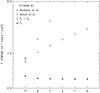 |
Fig. 3 Self-broadening parameter Γ for members of the Balmer line series. The widths (Γ3) from Ali & Griem (1965, 1966) follow a markedly different trend than widths from Barklem et al. (2000a). Improvements are obtained by adding a van der Waals term (Γ6) to Ali & Griem (1965, 1966): Γ3 + Γ6. |
Barklem et al. (2000a) also determined validity limits for the quasi-static framework of 35, 13, and 8 Å for Hα, β, and γ, respectively, at T = 4665 K, revealing potential difficulties with higher members of the Balmer line series.
To assess any possible systematic errors in the measurement of stellar parameters based on Balmer line profiles, we explored three different approaches to calculating synthetic Balmer line spectra. In the first approach, the Balmer line profiles from Hα to the series limit were computed using widths from Ali & Griem (1965, 1966) ΓAG alone, while in the second approach we combined AG and van der Waals widths, ΓAG,vdW. In the last approach, the line profiles from Hα to Hγ were computed using widths from Barklem et al. (2000a), ΓBPO, multiplied by factors of 0.75 and 1.0, again to assess uncertainties, while the upper Balmer lines were computed using ΓAG,vdW. The Voigt profiles including Doppler and self-broadening were convolved with Stark-broadened profiles from Lemke (1997).
3.2. Heavy element line profiles
The dominant broadening mechanism at ~6000 K is collision with hydrogen atoms, but the effect of Stark broadening is also included as it contributes significantly at ~8000 K.
For the broadening of Mg i, Al i, Ca i, and Ca ii lines caused by collisions with hydrogen atoms, we employed the coefficients of Barklem et al. (2000b), where the FWHM of the Lorentzian profiles is given by 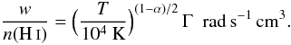 (3)For example, we adopted log Γ = −7.562 for Ca iλ4226 and log Γ = −7.76 for Ca H&K at T = 10 000 K, and α = 0.238 for Ca iλ4226 and α = 0.223 for Ca H&K. Stark broadening widths for Ca i and Ca ii lines were obtained from Dimitrijević & Sahal-Bréchot (1999) and Dimitrijević & Sahal-Bréchot (1992), respectively. Additional parameters (Stark and collisions with hydrogen) were obtained from the compilation of Kurucz & Bell (1995).
Hydrogen molecules provide ≲20% of the gas pressure in some layers of the models at Teff = 6000 K and a negligible fraction at 8000 K. Consequently, the effect of collisions with molecules is not considered further.
3.3. Effective temperature and surface gravity measurements
Fitting the V − J colour index to synthetic colours (Table A.1) constrains the effective temperature of the cool white dwarfs (Table 4). Within the error bars, the cooler objects are at Teff ≈ 6000 K, while NLTT 23966 is hotter with Teff ≈ 7600 K. These preliminary colour-based estimates are corroborated by our detailed Balmer line analysis.
We simultaneously constrained Teff and log g by fitting the X-shooter spectra with the model grids using χ2 minimization techniques. All lines up to the series limit, H8/9 for the cooler stars and H10 for NLTT 23966, are included in the analysis, but we excluded the Hϵ/Ca H blend in the three cooler stars. Figure 4 compares the Balmer line profiles of the four white dwarfs with the best-fit model spectra that were calculated using ΓAG,vdW.
Figure 5 illustrates the range of effective temperatures and surface gravities attained for the sample when employing different broadening parameters. Values connected with thin grey lines were obtained using either ΓAG alone (upper points), or ΓAG,vdW (lower points). The values connected with full black lines were obtained using ΓBPO (Hα,β,γ) combined with ΓAG,vdW for the upper Balmer lines (lower points), or reduced 0.75 × ΓBPO values combined with ΓAG,vdW (upper points). The derived parameters are compared to evolutionary cooling tracks (Benvenuto & Althaus 1999), allowing estimates of the mass and cooling age of each object.
The average mass of the three cooler stars computed using ΓAG,vdW line widths, is 0.53 M⊙. Similarly, the average mass is 0.57 M⊙ using the combination ΓBPO × 0.75/ΓAG,vdW. On the other hand, the average mass of 0.96 M⊙, obtained using ΓAG, appears improbably high, while the average mass of 0.44 M⊙, obtained using the combination ΓBPO/ΓAG,vdW, appears improbably low. Higher (lower) values of the surface gravity (hence density) are derived as a compensation for using smaller (larger) values of Γ. Considering the uncertainties in Γ, it seems appropriate to adopt an average mass near 0.6 M⊙ (see Tremblay et al. 2010) for the three cooler stars.
However, the surface gravity, hence mass, of NLTT 23966 is only marginally affected by variations in the self-broadening Γ value because of the dominant effect of Stark broadening at higher temperatures. The higher than average mass estimated for NLTT 23966 may also be attributed to the approximate treatment of convection in current model calculations (Tremblay et al. 2011).
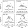 |
Fig. 4 Balmer line fits of X-shooter spectra using the line-broadening prescription ΓAG,vdW (see text). With the exception of NLTT 23966, the Hϵ/Ca H blend is excluded from the line fitting. |
Table 4 lists the adopted effective temperature and surface gravity of the cool white dwarfs. As a compromise, we adopted the average of the values obtained using model spectra calculated with ΓAG,vdW or ΓBPO × 0.75. Individual white dwarf masses were calculated following Benvenuto & Althaus (1999).
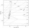 |
Fig. 5 Range of parameters (Teff vs. log g) determined for a sample of four cool hydrogen-rich white dwarfs using three different prescriptions for hydrogen line broadening (see text). The measured parameters are compared to evolutionary tracks from Benvenuto & Althaus (1999) with masses ranging from 0.3 to 1.0 M⊙, and ages ranging from 1 to 5 Gyr. An age discontinuity is apparent ~0.45 M⊙ because of the different core composition adopted for models with M ≤ 0.4 M⊙ (He) and M ≥ 0.5 M⊙ (C/O). |
Stellar properties.
3.4. Abundance of heavy elements
The abundances were computed at log g = 8.0 and Teff = 6000 ± 100 K for the cooler stars, and at log g = 8.25 and Teff = 7800 ± 100 K for NLTT 23966. Table 5 lists the measurements obtained by fitting the spectra with models of varying composition; the quoted errors include the (mild) effect of varying the temperature by ± 100 K, and the upper limits are taken at 99% certainty (2.6σ). However, the magnesium and aluminium abundances are based on ~2σ detections and higher S/N spectra would be required to improve the quality of these measurements. On the other hand, a strict upper limit to the calcium abundance in NLTT 23966 shows that its atmosphere is devoid of heavy elements. Figure 6 shows the various metal lines detected in NLTT 1675 compared to the best-fit model spectra.
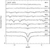 |
Fig. 6 X-shooter spectra of NLTT 1675 compared to the best fit model. The wavelength scale is centred on the values indicated on the right. The top two spectra show the weak Al i lines, followed by spectra showing Mg i lines around 3838 Å and 3832 Å and Fe i lines around 3740 Å and 3720 Å. Finally, the bottom three spectra show the Ca i and Ca ii lines. |
3.5. Radial velocity measurements, kinematics, and ages
We measured radial velocities νr = 15.0,83.2,64.2, and 66.4 km s-1 for NLTT 1675, 6390, 11393, and 23966, respectively. We estimated the error to be 5.0 km s-1 based on the scatter in individual line measurements and the expected precision of a R ~ 9000 spectrograph. Taking into account the expected gravitational redshift of the white dwarfs (based on the spectroscopically determined parameters), the actual velocities of the stars are ν = −16.5 ± 5.8,58.3 ± 5.8,40.9 ± 5.4, and 25.4 ± 5.4 km s-1 for NLTT 1675, 6390, 11393, and 23966, respectively.
Table 6 lists the cooling age, absolute magnitude, distance, and Galactic space velocities of the sample. The ages were computed using the evolutionary models of Benvenuto & Althaus (1999) and the absolute magnitudes were calculated using our model grid and radii from Benvenuto & Althaus (1999). The photometric distances were calculated using the apparent (Table 3) and absolute (Table 6) Johnson V magnitudes. Finally, the Galactic velocity components UVW were calculated using Johnson & Soderblom (1987). The lag in V suggest that the white dwarfs belong to the old thin disk (Sion et al. 1988; Pauli et al. 2003, 2006).
Age, distance, and kinematics.
3.6. Magnetic field strengths
A lack of splitting at the instrument resolution (R ~ 9000) imposes a limit on the magnetic field strength. Setting a limit of approximately one-third of a resolution element on the putative magnetic broadening of narrow line cores caused by Zeeman splitting: 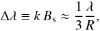 (4)where k = 4.67 × 10⁻¹³λ2 geff, λ is the wavelength in Å, Bs is the average surface field in G, and geff is the effective Landé factor (=
  and
and  for Ca K and H, respectively). For example, using the Ca K line observed in NLTT 1675, we estimate a limit on the magnetic field strength of Bs ≲ 17 kG. However, this effect could be confused with the effect of stellar rotation.
We obtained VLT/FORS spectropolarimetry for three stars (NLTT 6390, 11393, and 23966) in addition to NLTT 10480. We calculated the mean longitudinal magnetic (Bl in G) field using the weak-field approximation (Angel et al. 1973)  (5)where ν = V/I is the degree of circular polarization, F ≡ I is the total spectral flux, and dF/dλ is the flux gradient. First, we fitted the observed Balmer line profiles with model spectra to determine the best-fit line profiles. We then used these line profiles to calculate the flux gradient and determine the longitudinal magnetic field. To measure the longitudinal field strength for NLTT 6390 and NLTT 11393, we used Hβ to Hδ and for NLTT 23966 we used Hα.
Table 7 lists the longitudinal field measurements for three stars (NLTT 6390, 11393, and 23966) from this paper and for the cool white dwarf NLTT 10480 (Kawka & Vennes 2011). The quoted errors are 1σ. Using the Balmer lines, no fields stronger than ~5 to ~20 kG are detected in NLTT 6390, 11393, and 23966, but we measured a longitudinal field strength Bl = −200.4 ± 124.0 kG in NLTT 10480, which is barely a 2σ detection. The large uncertainty in Bl is mostly due to the weakness of the Balmer lines (Hβ, γ and δ) in NLTT 10480, but a measurement based on the calcium lines appears to be more reliable.
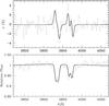 |
Fig. 7 Circular polarization (top) and flux (bottom) spectra of NLTT 10480. The observed circular polarization spectrum is compared to a model polarization spectrum at Bl = 212 kG (top). |
Equation (5) includes only the first term of a Taylor expansion that is used to calculate ν. This is valid where the Zeeman splitting is small relative to the line width. For Ca H&K in NLTT 10480, the Zeeman splitting is fully resolved, hence we need to include the second term of the Taylor expansion as described in Mathys & Stenflo (1986) (6)By fitting the Ca H&K circular polarization spectrum depicted in Kawka & Vennes (2011), we measured a longitudinal field of −212 ± 50 kG in NLTT 10480. Figure 7 shows the best-fit model circular polarization and flux spectra to the observed FORS spectra of NLTT 10480. A reasonable match is achieved between the model and observed spectra, except for the left σ component of the CaII λ3968 Å line, which appears stronger than the model. This is an improvement over the Balmer line measurements, but it still has a significantly larger uncertainty than the measurements obtained for the other white dwarfs in the sample. This is mainly because of the low S/N in the spectral region containing the Ca ii lines. Combining the measurement of the surface field of 519 ± 4 kG (Kawka & Vennes 2011) and the Ca H&K measurement of the longitudinal field in NLTT 10480 suggests an inclination ≲ 59°, in agreement with the angle of 60 ± 3° inferred from the strength of the calcium Zeeman-split lines determined in Kawka & Vennes (2011).
Magnetic field measurements (FORS).
4. Summary and discussion
We have presented a detailed model atmosphere analysis of high-quality spectroscopy of a sample of cool DA white dwarfs. We have shown that the atmospheres of NLTT 1675, NLTT 6390, and NLTT 11393 are contaminated with heavy elements. However, we have also shown that, in contrast to the DAZ white dwarf NLTT 10480, none of these three new DAZ white dwarfs harbour a magnetic field. We also refined our analysis of the magnetic field in NLTT 10480 and confirmed our original results (Kawka & Vennes 2011).
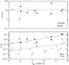 |
Fig. 8 Abundance ratio of iron with respect to calcium versus the effective temperature (top). The best fitting line that excludes NLTT 43806 is also shown. The abundance of iron and calcium versus the effective temperature (bottom), upper limits are not shown. The best fitting lines for iron (full line) and calcium (dashed line) are shown. |
Figure 8 shows the abundances of iron and calcium relative to hydrogen for a sample of cool DAZ white dwarfs, including those from the present sample, and the corresponding abundance ratio of iron with respect to calcium (Fe/Ca). The published abundance measurements were taken from Zuckerman et al. (2003) and Kawka et al. (2011), and from Farihi et al. (2011), Kawka & Vennes (2011), and Zuckerman et al. (2011) for the three magnetic white dwarfs, G77-50, NLTT 10480, and NLTT 43806, respectively. Table B.1 lists the selected measurements. The Fe/Ca abundance ratio appears to be constant as a function of temperature with an average of ⟨ Fe/Ca ⟩ = 13.1 and a dispersion of σ = 0.33 dex. The linear fit to the data excludes NLTT 43806, which has a Fe/Ca abundance ratio of ≈1.3 (Zuckerman et al. 2011), making it significantly iron-poor compared to the rest of the sample. Similarly, Fe/Al is ≈0.6 in NLTT 43806, while it is ≈4.5 in NLTT 1675. Both calcium and iron abundances exhibit an increase as a function of temperature, but the scatter in the iron abundance measurements (σ ~ 0.31 dex) is smaller than that of calcium (σ ~ 0.95 dex). It is possible that higher S/N and higher dispersion spectra of objects apparently devoid of iron would uncover even lower iron abundances and thereby increase the scatter in the measurements. In summary, the Fe/Ca abundance fraction is ~10 compared to ≈14 in the Sun. The Mg/Ca abundance fraction of NLTT 1675, NLTT 6390, G77-50, and NLTT 43806 range between ≈6 and ≈30.
Inferred accretion rates  (g s-1).
We have calculated the accretion rates assuming a steady state between accretion and diffusion for magnesium, aluminium, calcium, and iron. We have used the diffusion timescales and mass of the convective zone of Koester (2009). For aluminium, we used the diffusion timescale log τAl = 4.23 that Zuckerman et al. (2011) adopted for NLTT 43806, which is a star with temperature and surface gravity similar to our sample of DAZ white dwarfs. Table 8 lists the accretion rates for the NLTT 1675, 6390, and 11393. For objects with upper limits to their abundances, such as NLTT 23966, we listed the corresponding upper limits to the accretion rates. The observed abundance ratios relative to calcium in meteorites (C1 chondrites) or in the Sun (Grevesse et al. 2007) are log Mg/Ca,log Al/Ca,log Fe/Ca = 1.23, 0.10, and 1.15, respectively. Our sample appears to conform with these ratios. Following sample trends, magnesium and iron may well be present in NLTT 11393 but slightly below detection limits in our spectra.
For the whole sample, the observed calcium and iron abundances follow the expected temperature trend assuming a constant accretion rate over cooling ages (see Koester & Wilken 2006), although the trend appears steeper. The calcium and iron abundances increase by 0.32 dex and 0.4 dex per 1000 K interval, respectively, compared to the predicted increases of 0.26 dex and 0.27 dex per 1000 K interval assuming uniform accretion over the sample. This steeper trend suggests that the accretion flow onto white dwarfs may slightly diminish with time, or that the actual particle flux at the bottom of the convection zone may be underestimated in cooler, i.e., older white dwarfs.
Prior to this study, five DAZ white dwarfs with Teff ≲ 6000 K had been known, of which two of these, NLTT 43806 (Kawka & Vennes 2006) and NLTT 10480 (Kawka & Vennes 2011) had been discovered as part of our spectroscopic observations of white dwarf candidates from the rNLTT catalogue. In this paper, we have added three more cool DAZ white dwarfs to this important sample of accreting objects. We emphasize the notably high incidence of magnetism among this small sample of stars: three out of the eight DAZ white dwarfs cooler than ≈6000 K (G77-50, NLTT 43806 and NLTT 10480) are weakly magnetic. This incidence is markedly higher than previously estimated (Kawka et al. 2007; Liebert et al. 2003).
Following an inquiry by M. Jura, we found that sodium is not detected in any of our spectra. We calculated upper limits ranging from log(Na/H) = –9.5 to –9.0 or 2 to 10 times the solar Na/Ca ratio.
Online material
Appendix A: Synthetic Johnson and Sloan colours
Selected synthetic colours.
Appendix B: Abundance measurements
Abundance measurements of cool white dwarfs.
Acknowledgments
S.V. and A.K. are supported by GA AV grant numbers IAA300030908 and IAA301630901, respectively, and by GA ČR grant number P209/10/0967. A.K. also acknowledges support from the Centre for Theoretical Astrophysics (LC06014). We thank the referee, D. Koester, for helpful suggestions. This research has made use of the VizieR catalogue access tool, CDS, Strasbourg, France. This publication makes use of data products from the Two Micron All Sky Survey, which is a joint project of the University of Massachusetts and the Infrared Processing and Analysis Center/California Institute of Technology, funded by the National Aeronautics and Space Administration and the National Science Foundation.
References
- Ali, A. W., & Griem, H. R. 1965, Phys. Rev., 140, 1044 [NASA ADS] [CrossRef] [Google Scholar]
- Ali, A. W., & Griem, H. R. 1966, Phys. Rev., 144, 366 [NASA ADS] [CrossRef] [Google Scholar]
- Allard, N. F., Kielkopf, J. F., Cayrel, R., & van’t Veer-Menneret, C. 2008, A&A, 480, 581 [NASA ADS] [CrossRef] [EDP Sciences] [Google Scholar]
- Angel, J. R. P., McGraw, J. T., & Stockman, H. S., Jr. 1973, ApJ, 184, L79 [NASA ADS] [CrossRef] [Google Scholar]
- Barklem, P. S., Piskunov, N., & O’Mara, B. J. 2000a, A&A, 363, 1091 [NASA ADS] [Google Scholar]
- Barklem, P. S., Piskunov, N., & O’Mara, B. J. 2000b, A&AS, 142, 467 [NASA ADS] [CrossRef] [EDP Sciences] [MathSciNet] [PubMed] [Google Scholar]
- Benvenuto, O. G., & Althaus, L. G. 1999, MNRAS, 303, 30 [NASA ADS] [CrossRef] [Google Scholar]
- Berger, L., Koester, D., Napiwotzki, R., Reid, I. N., & Zuckerman, B. 2005, A&A, 444, 565 [NASA ADS] [CrossRef] [EDP Sciences] [Google Scholar]
- Bergeron, P., Wesemael, F., & Fontaine, G. 1991, ApJ, 367, 253 [NASA ADS] [CrossRef] [Google Scholar]
- Bessell, M. S. 1990, PASP, 102, 1181 [NASA ADS] [CrossRef] [Google Scholar]
- Dimitrijević, M. S., & Sahal-Bréchot, S. 1992, Bull. Astron. Belgrade, 145, 83 [NASA ADS] [Google Scholar]
- Dimitrijević, M. S., & Sahal-Bréchot, S. 1999, A&AS, 140, 191 [NASA ADS] [CrossRef] [EDP Sciences] [Google Scholar]
- Dufour, P., Bergeron, P., Schmidt, G. D., et al. 2006, ApJ, 651, 1112 [NASA ADS] [CrossRef] [Google Scholar]
- Farihi, J., Dufour, P., Napiwotzki, R., & Koester, D. 2011, MNRAS, 413, 2559 [NASA ADS] [CrossRef] [Google Scholar]
- Graham, J. R., Matthews, K., Neugebauer, G., & Soifer, B. T. 1990, ApJ, 357, 216 [NASA ADS] [CrossRef] [Google Scholar]
- Grevesse, N., Asplund, M., & Sauval, A. J. 2007, Space Sci. Rev., 130, 105 [Google Scholar]
- Johnson, D. R. H., & Soderblom, D. R. 1987, AJ, 93, 864 [NASA ADS] [CrossRef] [Google Scholar]
- Kawka, A., & Vennes, S. 2006, ApJ, 643, 402 [NASA ADS] [CrossRef] [Google Scholar]
- Kawka, A., & Vennes, S. 2011, A&A, 532, A7 [NASA ADS] [CrossRef] [EDP Sciences] [Google Scholar]
- Kawka, A., Vennes, S., & Thorstensen, J. R. 2004, AJ, 127, 1702 [NASA ADS] [CrossRef] [Google Scholar]
- Kawka, A., Vennes, S., Schmidt, G. D., Wickramasinghe, D. T., & Koch, R. 2007, ApJ, 654, 499 [NASA ADS] [CrossRef] [Google Scholar]
- Kawka, A., Vennes, S., Dinnbier, F., Cibulková, H., & Németh, P. 2011, AIP Conf. Ser., 1331, 238 [NASA ADS] [CrossRef] [Google Scholar]
- Koester, D. 2009, A&A, 498, 517 [NASA ADS] [CrossRef] [EDP Sciences] [Google Scholar]
- Koester, D., & Wilken, D. 2006, A&A, 453, 1051 [NASA ADS] [CrossRef] [EDP Sciences] [Google Scholar]
- Koester, D., Provencal, J., & Shipman, H. L. 1997, A&A, 230, L57 [NASA ADS] [Google Scholar]
- Koester, D., Rollenhagen, K., Napiwotzki, R., et al. 2005, A&A, 432, 1025 [NASA ADS] [CrossRef] [EDP Sciences] [Google Scholar]
- Koester, D., Voss, B., Napiwotzki, R., et al. 2009, A&A, 505, 441 [NASA ADS] [CrossRef] [EDP Sciences] [Google Scholar]
- Kowalski, P. M., & Saumon, D. 2006, ApJ, 651, L137 [Google Scholar]
- Kurucz, R. L., & Avrett, E. H. 1981, SAO Spec. Rep., 391 [Google Scholar]
- Kurucz R., & Bell B. 1995, Atomic Line Data Kurucz CD-ROM No. 23 (Cambridge MA: Smithsonian Astrophysical Observatory) [Google Scholar]
- Lacombe, P., Wesemael, F., Fontaine, G., & Liebert, J. 1983, ApJ, 272, 660 [NASA ADS] [CrossRef] [Google Scholar]
- Lemke, M. 1997, A&AS, 122, 285 [NASA ADS] [CrossRef] [EDP Sciences] [Google Scholar]
- Lépine, S., & Shara, M. M. 2005, AJ, 129, 1483 [NASA ADS] [CrossRef] [Google Scholar]
- Liebert, J., Bergeron, P., & Holberg, J. B. 2003, AJ, 125, 348 [NASA ADS] [CrossRef] [Google Scholar]
- Mathys, G., & Stenflo, J. O. 1986, A&A, 168, 184 [NASA ADS] [Google Scholar]
- Nordhaus, J., Wellons, S., Spiegel, D. S., Metzger, B. D., & Blackman, E. G. 2011, Proc. National Academy of Science, 108, 3135 [Google Scholar]
- Paquette, C., Pelletier, C., Fontaine, G., & Michaud, G. 1986, ApJS, 61, 197 [NASA ADS] [CrossRef] [Google Scholar]
- Patat, F., Moehler, S., O’Brien, K., et al. 2011, A&A, 527, A91 [NASA ADS] [CrossRef] [EDP Sciences] [Google Scholar]
- Pauli, E.-M., Napiwotzki, R., Altmann, M., et al. 2003, A&A, 400, 877 [NASA ADS] [CrossRef] [EDP Sciences] [Google Scholar]
- Pauli, E.-M., Napiwotzki, R., Heber, U., Altmann, M., & Odenkirchen, M. 2006, A&A, 447, 173 [NASA ADS] [CrossRef] [EDP Sciences] [Google Scholar]
- Potter, A. T., & Tout, C. A. 2010, MNRAS, 402, 1072 [NASA ADS] [CrossRef] [Google Scholar]
- Reid, I. N., Liebert, J., & Schmidt, G. D. 2001, ApJ, 550, L61 [NASA ADS] [CrossRef] [Google Scholar]
- Rohrmann, R. D., Althaus, L. G., & Kepler, S. O. 2011, MNRAS, 411, 781 [NASA ADS] [CrossRef] [Google Scholar]
- Salim, S., & Gould, A. 2003, ApJ, 582, 1011 [NASA ADS] [CrossRef] [Google Scholar]
- Sion, E. M., Fritz, M. L., McMullin, J. P., & Lallo, M. D. 1988, AJ, 96, 251 [NASA ADS] [CrossRef] [Google Scholar]
- Skrutskie, M. F., Cutri, R. M., Stiening, R., et al. 2006, AJ, 131, 1163 [NASA ADS] [CrossRef] [Google Scholar]
- Tremblay, P.-E., Bergeron, P., Kalirai, J. S., & Gianninas, A. 2010, ApJ, 712, 1345 [NASA ADS] [CrossRef] [Google Scholar]
- Tremblay, P.-E., Ludwig, H.-G., Steffen, M., Bergeron, P., & Freytag, B. 2011, A&A, 531, L19 [NASA ADS] [CrossRef] [EDP Sciences] [Google Scholar]
- Vernet, J., Dekker, H., D’Odorico, S., et al. 2011, A&A, 536, A105 [NASA ADS] [CrossRef] [EDP Sciences] [Google Scholar]
- Zuckerman, B., & Becklin, E. E. 1987, Nature, 330, 138 [NASA ADS] [CrossRef] [Google Scholar]
- Zuckerman, B., & Reid, I. N. 1998, ApJ, 505, L143 [NASA ADS] [CrossRef] [Google Scholar]
- Zuckerman, B., Koester, D., Reid, I. N., & Hünsch, M. 2003, ApJ, 596, 477 [NASA ADS] [CrossRef] [Google Scholar]
- Zuckerman, B., Koester, D., Dufour, P., et al. 2011, ApJ, 739, 101 [NASA ADS] [CrossRef] [Google Scholar]
All Tables
All Figures
|
Fig. 1 Identification spectra, fλ versus λ, normalized at λ = 5500 Å and shifted up for clarity. |
| In the text | |
|
Fig. 2 X-shooter spectra covering iron (left) and calcium (right) lines in four cool, hydrogen-rich white dwarfs from the NLTT catalogue. Photospheric calcium lines are observed in three stars, while iron was only observed in NLTT 1675 and 6390. In contrast to our initial report (Kawka et al. 2011), our new X-shooter spectra show that NLTT 23966 is devoid of calcium. The possible identification of aluminium is reported for NLTT 1675. |
| In the text | |
|
Fig. 3 Self-broadening parameter Γ for members of the Balmer line series. The widths (Γ3) from Ali & Griem (1965, 1966) follow a markedly different trend than widths from Barklem et al. (2000a). Improvements are obtained by adding a van der Waals term (Γ6) to Ali & Griem (1965, 1966): Γ3 + Γ6. |
| In the text | |
|
Fig. 4 Balmer line fits of X-shooter spectra using the line-broadening prescription ΓAG,vdW (see text). With the exception of NLTT 23966, the Hϵ/Ca H blend is excluded from the line fitting. |
| In the text | |
|
Fig. 5 Range of parameters (Teff vs. log g) determined for a sample of four cool hydrogen-rich white dwarfs using three different prescriptions for hydrogen line broadening (see text). The measured parameters are compared to evolutionary tracks from Benvenuto & Althaus (1999) with masses ranging from 0.3 to 1.0 M⊙, and ages ranging from 1 to 5 Gyr. An age discontinuity is apparent ~0.45 M⊙ because of the different core composition adopted for models with M ≤ 0.4 M⊙ (He) and M ≥ 0.5 M⊙ (C/O). |
| In the text | |
|
Fig. 6 X-shooter spectra of NLTT 1675 compared to the best fit model. The wavelength scale is centred on the values indicated on the right. The top two spectra show the weak Al i lines, followed by spectra showing Mg i lines around 3838 Å and 3832 Å and Fe i lines around 3740 Å and 3720 Å. Finally, the bottom three spectra show the Ca i and Ca ii lines. |
| In the text | |
|
Fig. 7 Circular polarization (top) and flux (bottom) spectra of NLTT 10480. The observed circular polarization spectrum is compared to a model polarization spectrum at Bl = 212 kG (top). |
| In the text | |
|
Fig. 8 Abundance ratio of iron with respect to calcium versus the effective temperature (top). The best fitting line that excludes NLTT 43806 is also shown. The abundance of iron and calcium versus the effective temperature (bottom), upper limits are not shown. The best fitting lines for iron (full line) and calcium (dashed line) are shown. |
| In the text | |
Current usage metrics show cumulative count of Article Views (full-text article views including HTML views, PDF and ePub downloads, according to the available data) and Abstracts Views on Vision4Press platform.
Data correspond to usage on the plateform after 2015. The current usage metrics is available 48-96 hours after online publication and is updated daily on week days.
Initial download of the metrics may take a while.