| Issue |
A&A
Volume 537, January 2012
|
|
|---|---|---|
| Article Number | L6 | |
| Number of page(s) | 4 | |
| Section | Letters | |
| DOI | https://doi.org/10.1051/0004-6361/201118571 | |
| Published online | 16 January 2012 | |
The narrow, inner CO ring around the magnetic Herbig Ae star HD 101412⋆
1 Department of Astronomy, University of Michigan, Ann Arbor, MI 48109-1090, USA
e-mail: This email address is being protected from spambots. You need JavaScript enabled to view it.
2 Leibniz-Institut für Astrophysik Potsdam (AIP), An der Sternwarte 16, 14482 Potsdam, Germany
3 Istituto Nazionale di Astrofisica, Osservatorio Astronomico di Trieste, via Tiepolo 11, 34143 Trieste, Italy
4 European Southern Observatory, Karl-Schwarzschild-Str. 2, 85748, Garching bei München, Germany
Received: 3 December 2011
Accepted: 23 December 2011
Abstract
We describe and model emission lines in the first overtone band of CO in the magnetic Herbig Ae star HD 101412. High-resolution CRIRES spectra reveal unusually sharp features which suggest the emission is formed in a thin disk centered at 1 AU with a width 0.32 AU or less. A wider disk will not fit the observations. Previous observations have reached similar conclusions, but the crispness of the new material brings the emitting region into sharp focus.
Key words: stars: individual: HD 101412 / stars: pre-main sequence / stars: magnetic field / stars: variables: general / circumstellar matter / protoplanetary disks
Based on observations obtained at the European Southern Observatory (ESO programme 087.C-0124(A)).
© ESO, 2012
1. Introduction
The star HD 101412 (V1052 Cen) has been referred to in numerous papers as a Herbig Ae star. It has an infrared excess, and a disk (cf. Fedele et al. 2008).
HD 101412 is most unusual in having resolved, magnetically split spectral lines which reveal a surface field modulus that varies between 2.5 to 3.5 kG (Hubrig et al. 2010). Salyk et al. (2011a) have surveyed molecular emission in a variety of young stellar objects. They found the emission to be much more subdued in Herbig Ae/Be stars than their cooler congeners, the T Tauri stars. This was true for HD 101412 as well, which was among the 25 Herbig Ae/Be stars they discussed. One exception, however, was the molecule CO2, which had a very large flux in HD 101412; indeed, only one T Tauri star had a higher CO2 flux.
In this Letter, we report observations of lines in the first overtone (v = 2 → 0) band of carbon monoxide (CO) in HD 101412. This feature has been the subject of previous studies (cf. Najita et al. 1996, and references therein), leading to conclusions in general agreement with those presented here.
Wheelwright et al. (2010) studied this band in 7 upper main-sequence stars with masses from 6 to 43 M⊙, significantly larger than that of HD 101412, ca. 2.5 M⊙ (Hubrig et al. 2009). Individual lines were not resolved, but models were constructed to fit the band head. The fits constrained the CO emission within limits of a few tenths of an AU (inner) to up to 8 AU (outer).
2. Observations and reductions
We present observations made with the ESO CRIRES spectrometer (Käufl et al. 2004) using a slit width of 0.2 arcsec. The achieved resolution was determined from weak telluric lines, and is slightly above 90 000. The signal to noise is difficult to obtain empirically because of strong and myriad weak telluric features. Local tests of the rms fluctuations in 1 to 3 Å regions (10 to 30 pixels) yield S/N between 100 and 200, averaging 153.
We discuss observations in two CRIRES regions, 2290–2301 nm, and 2303–2313.5 nm, made on 5 April 2011 at rotational phase 0.94 (Hubrig et al. 2011). The first of these regions contains the band head of  (henceforth, CO will mean this isotopologue). This head is located at 2292.8976 nm, the position of the rotational line R(51): (v′′ = 0,J′′ = 51 → v′ = 2,J′ = 52). (Note: The double prime refers to the lower level.)
Stellar (rest) wavelengths were determined using telluric and identified atomic stellar features, primarily C i, Mg i and Si i lines. These lines were measured in other CRIRES regions, covering 1065–1105 and 1585–1550 nm. The transformation to rest stellar wavelengths was then applied to the CO regions.
Telluric features were removed using hot standard stars with large rotational velocities, observed at comparable zenith distances. For the CO features, this procedure introduced both noise, and artifacts; it was necessary to judge the position of the continuum in both the target and standard stars. The minimum of the central M-feature is particularly sensitive to this subjective judgment (see Fig. 1).
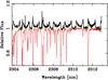 |
Fig. 1 The black spectrum shows CO emission lines R(20) (right) to R(27) (left) in HD 101412 after removal of telluric lines using the standard (red) star, HR 4537, j Cen. |
3. The CO emission lines and band head
3.1. Optically thick or thin?
We assume an optically thin emitting gas as a reasonable approximation. This is based on the sharpness of the profiles shown in Figs. 1 and 2. Self-absorption would smooth the sharp edges of the M-shaped profiles, filling in the centers, and spilling intensity over at the sides (edges) of the profiles. Additionally, we obtain a good fit to the band head using this assumption (Fig. 3). We can also make an estimate of the optical depth from the excess CO emission above the stellar continuum, using stellar parameters from Cowley et al. (2010) and Hubrig et al. (2009). The method is similar to that discussed by Salyk et al. (2011b), though we use a toroidal geometry for the emitting region rather than a slab. Plausible assumptions lead to an optical depth of 0.04 for R(20)1.
3.2. An empirical fit
All observations discussed here are in the R-branch of the first overtone band of the (X2Σ + ) ground electronic state of CO. Identifications of molecular features, and temperature-dependent predictions are based on the data file coxx.asc (Kurucz 1993). Only lines were considered. All others were assumed to be too weak to be relevant, or outside our limited observational regions.
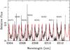 |
Fig. 2 Observed CO R(20)–R(27) in black. The observations are those of Fig. 1 (black). We subtracted unity, and scaled the remainder vertically to fit the observations. R-branch labels are written above the M-shaped profiles. Rest wavelengths of these lines correspond to the inner vertex of the M’s. R(19) is at the extreme right, but only the violet edge of the observed profile is seen. Several sharp spikes may be attributed to imperfect removal of the telluric features that may be seen in the standard star spectrum of Fig. 1. Red shows calculated molecular features for a temperature of 2500 K. |
Emission spectra (Figs. 2 and 3) were calculated with the help of Kurucz’s data. We assumed that emission flux profiles can be represented by Gaussian functions with central intensity I ∝ gfλ-3exp − χu/kT, where gf and χu are the oscillator strength and the excitation potential of the upper level of the CO transitions. We adopted T = 2500 K.
In many cases (see Sect. 4), one can determine a rotational temperature from the relative intensities of the individual lines (cf. Brittain et al. 2009). However, the relative intensities of R(20)–R(27) hardly change from T = 2000 to 3000 K, the range we believe appropriate (see below). A first calculation, using a single Gaussian profile for each line placed the emissions in the middle of the observed M-shaped profiles. Carr (2005) discusses the canonical, disk-model M-shaped profile. We eventually adopted a set of 21 Gaussians for each line, with 0.0666 nm FWHM (0.04 nm 1/e-width). They were weighted appropriately to reproduce the observed profiles (red, Fig. 2). The Gaussian at the center, therefore had the lowest weight. Other choices for the FWHM and number of Gaussians could give similar results. The fit is thus cosmetic, apart from the central wavelength matches, and the overall profile widths of the calculated features. These match very well the molecular wavelengths and the expected widths (see Sect. 4).
The velocity half-widths of the Gaussians, for a mean wavelength of 2309 nm is 47.8 km s-1. This value, uncertain by ≈ 2%, is in agreement with the Keplerian velocity 47.1 km s-1 used below in a disk-model fit to the profiles.
The strongest lines in the region of Fig. 2 are R(20)–R(27). However, higher-order lines, with wavelengths increasing for R(n > 51) fill in some of the region between the stronger features. These R(n > 51) lines diminish in intensity for increasing values of n.
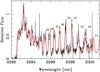 |
Fig. 3 First overtone band head with partially cosmetic fit. The assumed splitting and relative intensities (within a given M-shaped line) of the multiple Gaussian profiles are the same as in Fig. 2. The overall distribution of intensities is somewhat better fit by assuming T = 2500 K rather than 2000 or 3000 K. |
Figure 3 shows the region of the band head. Values of J′′ are written over the centers of the M-shaped profiles. Because of convergence to the head, vertical “sides” of the profiles approach one another, coincide, and eventually cross. Additionally, close to the head, transitions in the R-branch leading “away” (to the red) from the head (e.g. R(52)...R(56)) overlap and are of comparable intensity to the lines with R-values below that of the head, R(51).
The badly-blended head is reasonably well fit by the multi-Gaussian model. This indicates that the assumed profiles remain a good approximation for rotational lines somewhat higher than R(39). However, the relative importance of these higher-series lines diminishes rapidly. The R(51) line is 3.3 times weaker than R(31) at 2500 K.
The overall shape of the head region is more sensitive to the rotational temperature than the region of Fig. 2. By-eye fits to the observed features were best for temperatures between 2000 and 3000 K. The plot is for 2500 K, with an uncertainty of several hundred degrees.
4. A model emission ring
In this section we discuss a physical model to reproduce the M-shaped profiles. The code is far simpler than those used in some cited studies (e.g. Salyk et al. 2011b). The simplification is possible because we assume (1) the emitting gas is optically thin, (2) in pure Keplerian rotation, and (3) unobscured by the star or a dust disk.
The relevant code calculates the profile of a single emission line, and has not been adapted for multiple emissions, such as those shown in Figs. 2 and 3.
We constructed a two-dimensional model of the emission region, consisting of a set of 81 concentric rings, each with 288 emitting gas elements. They are all in Keplerian rotation around a 2.5 M⊙ star. The rings may be placed at arbitrary radial distances from the star. We assume that each element emits a Gaussian profile with a FWHM of 0.0666 nm.
A model that marginally fits the observations, has rings centered at 1 AU, spaced by 0.004 AU. This gives a disk 0.32 AU wide. A wider disk, at 1 AU, gives a profile that is too broad and rounded at the peaks to fit the observations. Indeed a single ring would produce an entirely satisfactory fit.
According to Fedele et al. (2008) the disk plane is 10° from the line of sight. Since cos(10°) = 0.985, we ignore the inclination, apart from the assumption that it must be enough for the emitting ring to be visible. A cosine factor may easily be incorporated, should future work reveal a larger inclination to the line of sight. Contributions from the 81 × 288 elements are Doppler shifted, added linearly, and scaled vertically to fit the observations.
Figure 4 shows a fit of the ring model to the rotational line R(20). The 81 rings are centered at 1 AU, and are separated by 0.001 AU.
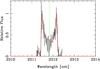 |
Fig. 4 Model fit (red) to the R(20) profile shown in Fig. 2. A thin, vertical line (green) marks the rest wavelength of R(20). The model is virtually a single ring, since rin = 0.96 and rout = 1.04 AU. |
Salyk et al. (2011b) stacked a number of their profiles in order to increase the signal to noise. We have attempted this in Fig. 5. The abscissa is rendered in velocity space. Plots have been scaled vertically for an optimum fit. The overall shape of the composite profile (black) is well fit by the model, apart from the low regions near the center of the “M” (thick, red). It is unclear how significant this is. We noted earlier the sensitivity of this portion of the profile to subjective judgments of the continuum location.
Additional emission is seen at the foot of the violet (or negative-V) side of the M-shaped profile. This is surely due to R-branch lines, R(J′′), where J′′ > 51. There is no provision in the model for this effect.
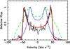 |
Fig. 5 Model fit to a composite of R(20) through R(27) of Fig. 2. The same parameters used for the fit of Fig. 4 (thick, red) give excellent agreement for the composite. Two additional curves illustrate profiles that would result from a wider disk (see text). |
Figure 5 shows two additional curves which illustrate the effect of an extended disk. Both curves assumed a disk with innermost rim at 0.4 AU, and outermost rim at 3.6 AU. The solid blue curve was made assuming each ring had the same total emissivity. The dashed green curve shows a profile where the emission is weighted by the negative 1.5th power of the radial distance. In this case, the innermost rings, with highest Keplerian velocities, have higher weights. This causes the additional emission at larger positive and negative velocities.
It is clear that such a disk cannot possibly account for sharply-edged rotational profiles. Quite elaborate radial intensity variations were considered by Acke et al. (2005, cf. their Fig. 21), in connection with [O I] emission. Happily, such complexity is unnecessary in the present case.
5. Discussion
Van der Plas et al. (2008), and Fedele et al. (2008) have discussed the protoplanetary disks around “three young intermediate mass stars”, including HD 101412, based on observations of forbidden oxygen, [O i] λ6300. They discuss disk models, though not as localized as the one that fits our CO observations.
Salyk et al. (2011b) studied the fundamental (v = 1 → 0) CO band in 31 T Tauri and Herbig Ae/Be stars, including a number with transitional disks. Rotational lines of the fundamental CO band are more commonly seen in T Tauri stars than the first overtone, the subject of the present paper. Salyk et al. conclude their line fluxes are “consistent with emission from a single temperature ring width 0.15 and 0.01 AU respectively...”. This conclusion is very close to that of the present paper. However, the profiles illustrated by Salyk et al. are much less sharply defined than those we observe in the first CO overtone in HD 101412. The central portions of their profiles are mostly filled in, indicating emission from regions of a disk beyond the innermost rim. Thus, they were also able to obtain fits (see their Table 4) with disk models extending over several and even tens of AU. The HD 101412 observations are incompatible with emission from such an extended disk.
Perhaps the T Tauri star with CO (fundamental) profiles most closely resembling the first overtone lines of HD 101412 is V836 Tauri (Najita et al. 2008). But note the sloping sides of their averaged profiles (their Figs. 4 and 5) in comparison to the nearly vertical sides of an analogous profile in HD 101412 presented below (Sect. 4).
The existence of narrowly-confined emission regions is well established. The current observations may be the best-defined example found thus far.
Details may be found at http://www.astro.lsa.umich.edu/~cowley/oldindex.html
Acknowledgments
C.R.C. thanks his Michigan colleagues for advice and support. Special thanks to Lee Hartmann for advice and encouragement. We acknowledge with thanks, the comments of Eric Mamajek.
References
- Acke, B., van den Ancker, M. E., & Dullemond, C. P. 2005, A&A, 436, 209 [NASA ADS] [CrossRef] [EDP Sciences] [Google Scholar]
- Brittain, S. D., Najita, J. R., & Carr, J. S. 2009, ApJ, 702, 85 [NASA ADS] [CrossRef] [Google Scholar]
- Carr, J. S. 2005, in High Resolution Infrared Spectroscopy in Astronomy, Proc. ESO Workshop held at Garching, Germany, ed. H. U. Käufl, R. Siebenmorgen, & A. Moorwood (Berlin: Springer), 203 [Google Scholar]
- Cowley, C. R., Hubrig, S., González, J. F., & Savanov, I. 2010, A&A, 523, A65 [NASA ADS] [CrossRef] [EDP Sciences] [Google Scholar]
- Fedele, D., van den Ancker, M. E., Acke, B., et al. 2008, A&A, 491, 809 [NASA ADS] [CrossRef] [EDP Sciences] [MathSciNet] [Google Scholar]
- Hubrig, S., Stelzer, B., Schöller, M., et al. 2009, A&A, 502, 283 [NASA ADS] [CrossRef] [EDP Sciences] [Google Scholar]
- Hubrig, S., Schöller, M., Savanov, I., et al. 2010, AN, 331, 361 [Google Scholar]
- Hubrig, S., Mikulášek, Z., González, J. F., et al. 2011, A&A, 525, L4 [NASA ADS] [CrossRef] [EDP Sciences] [Google Scholar]
- Käufl, H.-U., Ballester, P., Biereichel, P., et al. 2004, SPIE, 5492, 1218 [Google Scholar]
- Kurucz, R. L. 1993, CD-ROM No. 18, Smithsonian Astrophysical Observatory [Google Scholar]
- Najita, J., Carr, J. S., Glassgold, A. E., et al. 1996, ApJ, 462, 919 [NASA ADS] [CrossRef] [Google Scholar]
- Najita, J. R., Crockett, N., & Carr, J. S. 2008, ApJ, 687, 1168 [NASA ADS] [CrossRef] [Google Scholar]
- Salyk, C., Pontoppidan, K. M., Blake, G. A., Najita, J. R., & Carr, J. S. 2011a, ApJ, 731, 130 [NASA ADS] [CrossRef] [Google Scholar]
- Salyk, C., Blake, G. A., Boogert, A. C., & Brown, J. M. 2011b, ApJ, 743, 112 [NASA ADS] [CrossRef] [Google Scholar]
- van der Plas, G., van den Ancker, M. E., Fedele, D., et al. 2008, A&A, 485, 487 [NASA ADS] [CrossRef] [EDP Sciences] [Google Scholar]
- Wheelwright, H. E., Oudmaijer, R. D., de Wit, W. J., et al. 2010, MNRAS, 408, 1840 [NASA ADS] [CrossRef] [Google Scholar]
All Figures
|
Fig. 1 The black spectrum shows CO emission lines R(20) (right) to R(27) (left) in HD 101412 after removal of telluric lines using the standard (red) star, HR 4537, j Cen. |
| In the text | |
|
Fig. 2 Observed CO R(20)–R(27) in black. The observations are those of Fig. 1 (black). We subtracted unity, and scaled the remainder vertically to fit the observations. R-branch labels are written above the M-shaped profiles. Rest wavelengths of these lines correspond to the inner vertex of the M’s. R(19) is at the extreme right, but only the violet edge of the observed profile is seen. Several sharp spikes may be attributed to imperfect removal of the telluric features that may be seen in the standard star spectrum of Fig. 1. Red shows calculated molecular features for a temperature of 2500 K. |
| In the text | |
|
Fig. 3 First overtone band head with partially cosmetic fit. The assumed splitting and relative intensities (within a given M-shaped line) of the multiple Gaussian profiles are the same as in Fig. 2. The overall distribution of intensities is somewhat better fit by assuming T = 2500 K rather than 2000 or 3000 K. |
| In the text | |
|
Fig. 4 Model fit (red) to the R(20) profile shown in Fig. 2. A thin, vertical line (green) marks the rest wavelength of R(20). The model is virtually a single ring, since rin = 0.96 and rout = 1.04 AU. |
| In the text | |
|
Fig. 5 Model fit to a composite of R(20) through R(27) of Fig. 2. The same parameters used for the fit of Fig. 4 (thick, red) give excellent agreement for the composite. Two additional curves illustrate profiles that would result from a wider disk (see text). |
| In the text | |
Current usage metrics show cumulative count of Article Views (full-text article views including HTML views, PDF and ePub downloads, according to the available data) and Abstracts Views on Vision4Press platform.
Data correspond to usage on the plateform after 2015. The current usage metrics is available 48-96 hours after online publication and is updated daily on week days.
Initial download of the metrics may take a while.