| Issue |
A&A
Volume 537, January 2012
|
|
|---|---|---|
| Article Number | A85 | |
| Number of page(s) | 8 | |
| Section | The Sun | |
| DOI | https://doi.org/10.1051/0004-6361/201117851 | |
| Published online | 12 January 2012 | |
Magnetic and velocity fields of a solar pore
1 Astronomical Institute, Academy of Sciences of the Czech Republic (v.v.i.), Fričova 298, 25165 Ondřejov, Czech Republic
e-mail: This email address is being protected from spambots. You need JavaScript enabled to view it.
2 Department of Physics, University of Roma Tor Vergata, via della Ricerca Scientifica 1, 00133 Roma, Italy
Received: 8 August 2011
Accepted: 18 November 2011
Abstract
Context. Solar pores are intermediate-size magnetic flux features that emerge at the surface of the Sun. The absence of a filamentary penumbra indicates that there is a relatively simple magnetic structure with a prevailing vertical magnetic field.
Aims. Relations between the magnetic field components, line-of-sight velocities, and horizontal motions in and around a large pore (Deff = 8''.5) are analysed to provide observational constraints on theoretical models and numerical simulations.
Methods. Spectropolarimetric observations in Fe I 617.3 nm of the pore NOAA 11005 with the IBIS spectrometer attached to the Dunn Solar Telescope are inverted into series of maps of thermal, magnetic, and velocity parameters using the SIR code. Horizontal velocities are obtained from series of white-light images by means of local correlation tracking.
Results. The magnetic field B extends from the visible pore border of more than 3''.5 and has a radial structure in a form of spines that are co-spatial with dark intergranular lanes. The horizontal component Bhor is more extended than the vertical component Bz. The temperature linearly decreases with increasing Bz, by about − 300 K kG-1 in the photosphere and − 800 K kG-1 in the umbra. The temperature contrast of granulation increases with increasing magnetic field strength and is then suppressed for Bz > 1200 G. Granular upflows dominate in regions with Bz < 600–700 G. Line-of-sight velocities are lower in stronger fields, except for fast isolated downflows at the pore’s border. The velocity signature of granulation is suppressed completely for Bhor > 1000 G. Horizontal motions of granules start to be damped for Bz > 500 G and recurrently exploding granules appear only in magnetic fields comparable to or weaker than the equipartition field strength 400 G.
Key words: sunspots / Sun: photosphere
© ESO, 2012
1. Introduction
Pores are intermediate-size elements of a class of magnetic-flux features that emerge at the surface of the Sun. These elements range from well-known sunspots that measure up to 40 Mm in diameter with a field strength of up to several kG, to first pores with a size of a few Mm and a field strength of up to 2 kG, and then to small-scale magnetic flux tubes with a size comparable to, or even smaller than, our present ability to resolve fine details on the solar surface. For a review of pores and sunspots, we refer to e.g. Sobotka (2003) and Thomas & Weiss (2004).
The absence of a filamentary penumbra in the pores has been interpreted as an indication of a simple magnetic structure of a magnetostatic flux tube with a vertical field (e.g. Simon & Weiss 1970; Rucklidge et al. 1995). However, high spatial-resolution observations indicate that pores contain a wide variety of fine bright features, such as umbral dots or light bridges that may be signs of a convective energy transportation mechanism (e.g. Sobotka et al. 1999; Keil et al. 1999; Hirzberger 2003; Giordano et al. 2008; Sobotka & Jurčák 2009; Ortiz et al. 2010).
The determination of the physical origin of these fine structures is critical to understanding the sub-photospheric structure of sunspots and pores. Two categories of theoretical models have been found to be consistent with observations: a monolithic and inhomogeneous flux tube with embedded magnetoconvection (e.g. Hurlburt & Rucklidge 2000; Thomas & Weiss 2004, and references therein) and a bundle of spaghetti-like flux tubes (e.g. Parker 1979; Choudhuri 1986). Although based on different concepts, both models permit the presence of small and bright features embedded in the dark umbra.
Across a pore, the magnetic field strength varies from 600 G to 1700 G, as reported by Sütterlin et al. (1996) – cf. also Keppens & Martínez Pillet (1996) and Sütterlin (1998). Magnetic field lines are found to be nearly vertical at the centres of pores and inclined by about 40° to 80° at their edges. MHD simulations forecast that intense downflows, driven by an extra radiative cooling of the plasma and fed by horizontal flows in the upper layers, should surround the pores. For instance, the simulation by Cameron et al. (2007) reported a downflow of 1.5 km s-1 just outside the edge of the pore in the azimuthally averaged profile of the vertical velocity.
Equipartition between the kinetic and magnetic energy densities occurs when the Lorentz force is strong enough to counteract the convective motion. In particular, the equipartition magnetic field strength  , where ρ is the density, μ the magnetic permeability, and u the typical velocity of motion. At the solar surface, ρ = 3 × 10⁻⁴ kg m-3 and u = 2 km s-1 in granules. Therefore, Be = 400 G (Stix 1989). This value might be important as we search for relations between magnetic and velocity fields in the photosphere.
In this paper, we focus on magnetic and velocity fields in the active region NOAA 11005, which is a large solar pore with a light bridge. In particular, we investigate the relations between the magnetic and velocity fields in the pore and in its surroundings, attempting to provide observational constraints on theoretical models and numerical simulations.
The organisation of the paper is the following. In Sect. 2, we describe the observations, data processing, and the procedure used to obtain horizontal velocity maps. The spectropolarimetric data inversion is described in Sect. 3. In Sect. 4, we give the general characteristics of the pore. In Sect. 5, we study the relations between magnetic and velocity fields in the pore and its surroundings. In Sects. 6 and 7, we illustrate the magnetic field and the line-of-sight (LOS) and horizontal velocity fields around the pore. Concluding remarks are given in Sect. 8.
2. Observations and data processing
A large solar pore (NOAA 11005) was observed with the Interferometric Bidimensional Spectrometer (IBIS, Cavallini 2006) attached to the Dunn Solar Telescope (DST) on 15 October 2008 from 16:34 to 17:43 UT. During the observations, the seeing conditions varied from good to fair, but the high contrast of the pore allowed us to use it as lock-point for the wavefront sensor. Therefore, the adaptive optics (AO) system of the NSO/DST (Rimmele et al. 2004) achieved a good performance in terms of stability and resolution in the centre of the field of view (FOV). In this work, we use only of the central part of the IBIS FOV, since the spatial resolution and the image contrast degrade towards the edge of the FOV owing to the strong anisoplanatism (Fried 1982).
The active region NOAA 11005, according to the BASS 2000 data base1, was present on the solar disc from 11 to 16 October 2008. The slowly decaying pore, located at 25.2 N and 10.0 W during our observation, was a leader of a bipolar active region, where the following magnetic polarity was too weak to produce sunspots or pores.
The IBIS dataset consists of 80 sequences, each containing a full Stokes (I,Q,U,V) 21-point scan of the Fe I 617.33 nm line and a 21-point I-scan of the Ca II 854.2 nm line. The wavelength distance between the spectral points for the Fe I line is 2.0 pm (and 6.0 pm for the Ca II line). The spectropolarimetric data acquisition strategy that we used was to acquire six modulation states I + S (and their orthogonal states I − S) at each wavelength position: S = [ + Q, + V, − Q, − V, − U, + U ] . Each sequence threfore consists of 21 × 6 (Fe I) + 21 (Ca II) = 147 narrowband images. The exposure time for each image was set to 80 ms and each spectral scan took 52 s to complete, thus setting the time resolution. The pixel scale of these 512 × 512 pixel images was set to 0 167.
167.
The properties of the line Fe I 617.33 nm have been discussed by several authors (e.g. Landi Degl’Innocenti 1982; Solanki & Stenflo 1985). In the literature (cf. Norton et al. 2006), the line-formation height varies approximately from 250 to 350 km, depending on the adopted approach and model atmospheres. Its excitation potential is 2.22 eV and its effective Landé factor is geff = 2.5. The nearby continuum is clean (the nearest line is the 3F3-3F2 La II transition at 617.27 nm) and the line shows no blends with other solar or telluric lines in the quiet Sun. Only in the cooler atmosphere of a sunspot umbra, the Eu II 617.30 nm line shows up as a weak blend in the blue wing of Fe I 617.33 nm and two other weak lines appear in the nearby continuum (Norton et al. 2006). Those properties guarantee a very good performance for vector magnetic field retrieval, as is confirmed by its choice for the SDO/HMI instrument.
For each spectral image, we acquired a white-light (WL) and a G-band counterpart, approximately imaging the same field of view. The pixel scale of the 1024 × 1024 pixel WL image (621.3 ± 5 nm) was set to 00835 and the acquisition time was 80 ms (a shared shutter with IBIS spectral images). The pixel scale of the 1024 × 1024 pixel G-band image (430.5 ± 0.5 nm) was set to 00514 and the integration time to 10 ms.
For each sequence of the dataset, three MFBD (multi-frame blind deconvolution, van Noort et al. 2006) restored images, each computed from 49 original images, were obtained for both the WL and G-band channels. Forty-nine images are a good compromise between restoration quality, repeatability, and computation time. This also allowed us to reject a few restored images with artefacts yet still derive a high quality image for each sequence. The best restored WL image in each scan (with the highest contrast) was used as a reference to align and de-stretch the original WL images.
Since the wavelength difference between the WL and the Fe I 617.33 nm spectro-polarimetric images is less than 5 nm and the images share the same exposition instants, we were able to assume that their shifts and distortion caused by the seeing were equal. The corrections computed for the original WL images were therefore applied to their spectro-polarimetric counterparts via the de-stretching technique.
We then applied the standard reduction pipeline (Viticchié et al. 2010) on the spectro-polarimetric data, correcting for the instrumental blueshift (Cavallini 2006) and the instrument- and telescope-induced polarisations. The de-stretching applied to the Fe I 617.33 nm spectro-polarimetric images minimised the degradation of the spectro-polarimetric scan caused by image motion and distortion.
To calibrate the wavelength position of the scan, i.e., the LOS velocities, we computed the time- and space-averaged Fe I 617.33 nm line profile in the pore’s umbra. The core position of this profile was taken as the zero-velocity reference for the spectro-polarimetric scans.
An analysis of image quality was carried out to estimate the spatial resolution of the reduced dataset. In particular, we estimated the resolution of LOS velocity maps and LOS magnetograms derived from the dataset. Owing to the anisoplanatism effect, the resolution of the spectro-polarimetric data varied within the FOV. Nevertheless, the average resolution in the region near the tracking point of the AO system was better than 0 4 at any instant of our observation. The spectral stray light contaminating the dataset was estimated via comparison with the FTS atlas (Neckel 1999). The FTS spectrum was convolved with the IBIS spectral point-spread function at 617.33 nm, considering a certain amount of the spectral stray light as a free parameter. The optimal match between the acquired average line profile and the convolved FTS spectrum is obtained with the spectral stray-light contamination of between 1% and 2%.
The horizontal motions of granules around the pore were studied using the method of local correlation tracking (LCT, November & Simon 1988). Applied to a time series of images, LCT provides a time-averaged horizontal velocity field of all intensity structures. We must keep in mind that such velocity field may not reflect the real flow of gas. On the other hand, the motions of granules do trace horizontal photospheric flows caused by subsurface convection including its interaction with local magnetic fields (Simon et al. 1988). We used the time series of MFBD-restored WL images filtered by a k–ω Fourier filter with a cutoff of 5 km s-1 to remove image jitter and the effects of p-mode oscillations. The FWHM of the Gaussian tracking window was set to 075 (approximately a half of the granule size) and the temporal integration was made over an interval of 9.5 min, containing 33 restored WL frames aligned with the IBIS FOV. Four of these intervals were taken during the period of the highest image quality from 16:59 to 17:37 UT and four consecutive flow maps, including the divergence of horizontal velocity components, were computed.
3. Spectral data inversion
We used the inversion code SIR (Stokes Inversion based on Response functions, Ruiz Cobo & del Toro Iniesta 1992) to retrieve plasma properties in the Fe I 617.3 nm line-forming region. This code works under the assumption of local thermodynamical equilibrium and hydrostatic equilibrium. It starts with an initial model atmosphere, which is modified in several node points for each inverted plasma parameter to obtain the best fit of the synthetic Stokes profiles to the observed ones. The nodes correspond to certain heights in the atmosphere and their number determines the number of free parameters. Since the spectropolarimetric information comes from only one spectral line, we needed to keep the number of free parameters as small as possible. We enabled two nodes of temperature and one node of LOS velocity, magnetic field strength, field inclination, and azimuth – altogether, six free parameters. Microturbulent velocity was fixed at 1.3 km s-1.
The inversions were made for a single-component model atmosphere, i.e., the filling factor was unity. However, the spectra are contaminated by spatial stray-light (far wings of the point spread function), originating in both the instrument and the Earth’s atmosphere. We used the average Stokes I profile from the whole field of view as the profile of the spatial stray-light. In the SIR code, the amount of stray light can be a free parameter in the inversion process. We used a number of fixed values of stray light from 1% to 40% for tentative inversions of the highest-quality scan and obtained the closest match of synthetic and observed profiles for the spatial stray-light contamination of 15%. This value was then used for all inversions. The IBIS instrumental profile was also taken into account. There are many different methods for determining spatial stray-light in solar observations. The results depend on the instrumental complexity and the adopted method and may differ dramatically. For example, Wedemeyer-Böhm (2008) used the Mercury transit to find the upper limit to the stray light in the Hinode/SOT broadband imager (8% at a distance of 5′′, λ 668 nm) and Scharmer et al. (2011) compared observations with numerical simulations of granulation to determine the stray-light contamination in the SST/CRISP spectropolarimeter (58% of local stray light, λ 538 nm). Our method, based on tentative inversions, might suffer from an ambiguity in the inversion process. However, this ambiguity is limited in our case by the small number of free inversion parameters.
As a result of the inversion, for each of the 80 scans we obtained maps of temperature T, LOS velocity vLOS, magnetic field strength B (supposing that the filling factor is equal to one, otherwise B is the magnetic flux density), magnetic field inclination γ to the normal, and azimuth Φ in the FOV 20′′ × 167 (120 × 100 pixels). Owing to the one-node setting, vLOS, B, γ, and Φ are constant with optical depth τ and are considered to describe the typical physical conditions at τ = 0.03–0.1 (Cabrera Solana et al. 2005). The temperature is averaged over the range τ = 0.32–0.63. In this way, we obtained time series of two-dimensional maps of each physical parameter for further analysis.
As only one line was inverted, the precision of retrieved values of plasma parameters was limited. The uncertainties were also provided by the inversion code SIR; they are proportional to the achieved precision of the fit and disproportional to the sensitivity of the Stokes profiles to the given plasma parameter (see e.g. del Toro Iniesta 2003). The errors in the parameters corresponding to a single resolution element are on average ± 80 K in the temperature, ± 8° in magnetic field inclination, ± 120 G in magnetic field strength, and ± 320 m s-1 in LOS velocity. The largest uncertainties in T ( ± 180 K) and B ( ± 260 G) appear in the central parts of the pore, because the crosstalk between these plasma parameters is effective there. The maximum uncertainties in vLOS ( ± 450 m s-1) and γ ( ± 20°) were reached on the southwest boundary of the pore, where the fastest LOS flows were found.
We calculated components of the magnetic field vector B, namely the LOS component BLOS, vertical component Bz, and horizontal component  . For this purpose, we transformed the magnetic field inclination and azimuth from the LOS frame to the local reference frame. We first solved the 180° azimuth ambiguity by assuming that the magnetic field azimuth retrieved in and around the pore is close to the azimuth of the radially opening lines from the centre of the pore. We then used routines from the AZAM code developed for the Advanced Stokes Polarimeter (Lites et al. 1995) to transform the values of magnetic field azimuth and inclination to the local reference frame.
The seeing was variable during the 69-min observing period, such that the scans differed in spatial resolution and residual image deformation that was not corrected by the adaptive optics and de-stretching. To remove both image jitter and the effects of p-mode oscillations, and homogenise the data, each time series of maps was filtered by a k–ω Fourier filter with a cutoff 5 km s-1.
Fluctuations in the spatial resolution caused by seeing introduce random errors in individual maps of physical parameters. Since the pore did not show any significant evolutionary changes during the observing period, we attempted to remove the random errors by averaging the maps in time. Four averaging 9.5-min intervals, each including 11 scans, were taken during the period of highest image quality from 16:59 UT to 17:37 UT. These intervals are identical to those used for the LCT computation of horizontal flow maps. The averaging time is slightly longer than the characteristic lifetime of individual granules. Nevertheless, the average WL images (see example in Fig. 2) show a well-preserved granular structure, such that we can expect that the magnetic and flow structures around the pore are not influenced substantially by the averaging. In this way we obtained four sets of maps of time-averaged intensity, temperature, magnetic-field vector, LOS velocity, and apparent horizontal velocity.
4. General characteristics of the pore
The pore (Fig. 1) was located at the heliocentric position μ = 0.92 during the observation. A strong granular light bridge (LB) separated the pore into two umbral cores; the larger one was in the east. Minimum temperatures retrieved from inversions in the larger and smaller umbral cores were 4400 K and 4700 K, respectively. The effective diameter of the pore calculated from its area A including LB was  5 (6200 km). The umbral area (without LB) was practically constant during the observing period.
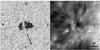 |
Fig. 1 Pore in NOAA 11005 observed on 15 October 2008 at 17:14 UT. Left – white-light image, right – Ca II 854.2 nm line-centre image. The field of view is 39′′ × 39′′, centred at the position 25.2 N 10.0 W; a black arrow indicates the direction to the disc centre. Symbols “+” and “ × ” mark the positions of the maximum magnetic field strength and its horizontal component, respectively. |
Continuum (WL) images show numerous umbral dots within both umbral cores (Fig. 1). However, no magnetic and Doppler velocity signatures of umbral dots are seen in the corresponding maps of B and vLOS. This is because at the formation height of the Fe I 617.3 nm line, the variation in the magnetic and Doppler velocity signals connected with umbral dots are too weak to be detected (cf. Sobotka & Jurčák 2009). Images in the Ca II 854.2 nm line show granule-like structures in LB and a large asymmetric filamentary (fibril) structure around the pore that extends to the west and north (Fig. 1).
The highest magnetic field strength B was found in the eastern (large) core near its northern (limbward) edge (Fig. 1). Its value increased with time from 1900 G to a maximum of 2100 G, which was reached at 17:18 UT. The vertical component Bz was strongest in the central region of the large core and its value increased with time from 1800 G to a maximum 2000 G at 17:18 UT and then decreased back to 1800 G. The maximum of the horizontal component Bhor was located at the western edge of the small umbral core and increased steadily from 1300 G to 1400 G.
The general geometry of the magnetic field was determined by means of an analysis of magnetic field inclination and azimuth at the pore’s edge. The method was described by Jurčák (2011). The magnetic field of the pore is, as a whole, inclined to the west by 10°, i.e., the axis of the field, which would be expected to be perpendicular to the surface, is instead inclined westward by 10° from the normal, away from the rest of the active region. The westward inclination is confirmed by the shape of the filamentary structure observed in the Ca II line-centre (Fig. 1). If this overall inclination is removed, the average magnetic field inclination at the pore’s edge is 40°, which is consistent with former observations (Keppens & Martínez Pillet 1996; Sütterlin 1998).
5. Relations between magnetic field, velocity fields, and temperature
Our main aim has been to study the relations between the magnetic and velocity fields in the pore and in its vicinity. We use four sets of time-averaged maps of physical parameters obtained by means of the inversion procedure and LCT (see Sect. 3). An example of the maps is shown in Fig. 2; an example of the LCT horizontal velocity map is shown in Fig. 3. Several well-known results can be seen in the figures: (i) the magnetic field extends beyond the visible edge of the pore (first observed by Keppens & Martínez Pillet 1996); (ii) the LOS velocities, clearly seen in the granulation, are suppressed inside the pore edge except for small-scale isolated downflow patches at the pore’s edge (Hirzberger 2003). The strongest downflows are seen at the southern border of the large core; (iii) the pore is surrounded by numerous divergence centres of horizontal motions formed by exploding granules (Sobotka et al. 1999).
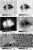 |
Fig. 2 Time-averaged grey-scale maps of physical parameters obtained for the period 17:09–17:18 UT. The field of view is 20′′ × 16 |
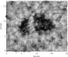 |
Fig. 3 Map of LCT horizontal velocities for the period 17:09–17:18 UT. We have superimposed the white-light image. The length of the black horizontal bar at the bottom left corner represents 1 km s-1. |
We separated the field of view into three regions using binary masks: the photospheric granulation, the light bridge, and the umbra. The umbra is defined as a region with WL intensity lower than 0.8 Iph, where Iph is a mean intensity of photospheric granulation in WL images. Ranges (minimum-to-maximum values) of magnetic field strength B and its LOS, vertical, and horizontal components BLOS, Bz, and Bhor, respectively, in the three regions are shown in Table 1.
Ranges of time-averaged magnetic field strength and its components.
For each region separately, we calculated the mean and standard deviation σ of temperature, LOS velocity, and horizontal velocity magnitude vhor in points (positions in FOV) with magnetic field falling into 50-G bins of histograms of BLOS, Bz, and Bhor. In this way, we obtain statistical relations between these parameters and magnetic field, namely, graphs of mean T and σT versus (vs.) Bz and Bhor, vLOS and σvLOS vs. BLOS and Bhor, and, finally, vhor and σvhor vs. Bz and Bhor. An example of the graphs for the period 17:09–17:18 UT is shown in Fig. 4. The relations, derived from the graphs of all four averaging periods, are described in Sects. 5.1–5.3.
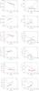 |
Fig. 4 Graphs of relations between temperature T, LOS velocity vLOS, horizontal velocity vhor and magnetic field components BLOS, Bz, and Bhor. Left – mean values, right – σ values. Black line – photospheric granulation, red (thick) – light bridge, green (grey) – umbra. |
5.1. Temperature
The temperature decreases with increasing vertical magnetic-field component Bz practically linearly (Fig. 4a), about − 300 K kG-1 in the photosphere, − 350 K kG-1 in the light bridge, and the steepest decrease − 800 K kG-1 is in the umbra. This is a consequence of the lower convective heat transfer in the vertical magnetic field. Temperature variations, characterised by the standard deviation σT (Fig. 4b), are at their strongest in the umbra because of the presence of umbral dots. In the photosphere, temperature fluctuations caused by granulation first increase until Bz = 1200 G (a typical value at the pore’s boundary) and then drop abruptly. This can be explained by the increasing width of the intergranular lanes in magnetised granulation and by the suppression of the granulation pattern for Bz > 1200 G. Temperature fluctuations in the light bridge are small and do not depend on Bz.
The temperature in the photospheric granulation decreases with increasing horizontal component Bhor (Fig. 4c). In the umbra, the temperature increases because Bhor is highest at the umbral periphery. The LB temperature increases with Bhor because the eastern part of the bridge is hotter and has a more inclined field (Fig. 2) owing to the stronger B in the eastern umbral core and the overall field inclination to the west. Temperature variations in granulation (Fig. 4d) increase upto Bhor = 1000 G (a typical value at the pore’s boundary) and then decrease.
5.2. Line-of-sight velocity
The LOS velocity was compared to the BLOS component (Fig. 4e). In the photosphere, granular upflows dominate the weak LOS magnetic field (BLOS < 600–700 G). The granular upflow overshoot to the formation height of Fe I 617.3 nm is suppressed in stronger fields, where no flows or 1–2 strong local downflows at the southern umbral edge are seen. No flows are observed in the umbra. In the light bridge, the character of flows is the opposite of that in the photosphere: downflows in the weaker field (BLOS < 900 G) and weak upflows or zero in the stronger BLOS. This may be a consequence of the individual characteristics of this particular LB: downflows appear in its northern part, where the magnetic field is weaker (cf. Fig. 2). The vLOS variations, characterised by σvLOS (Fig. 4f), are small (<100 m s-1) in the umbra and LB. In the photospheric granulation, the vLOS variations decrease with increasing BLOS until 800 G, owing to the reduction of convective motions. Local downflows at the pore’s edge induce an increase in the vLOS fluctuations for stronger field.
Comparing the LOS velocity with the Bhor component (Fig. 4g), we found that in the photosphere, granular upflows dominate the weak horizontal magnetic field (Bhor < 500–700 G). Weak downflows or no flows at all are observed for stronger Bhor. This behaviour is similar to the dependence of vLOS on BLOS. The vLOS variations in the photosphere (Fig. 4h) decrease with increasing horizontal field component for Bhor > 400 G and are smaller than 100 m s-1 for Bhor > 1000 G.
5.3. Horizontal velocity
The dependence of horizontal velocity on magnetic field components Bz and Bhor (Figs. 4i,k) is unclear and quite different in individual time-averaging periods. The only relation was found between vhor variations and Bz in granulation (Fig. 4j), where σvhor decreases with Bz > 500 G. In agreement with results of Keil et al. (1999), vhor is obviously much higher in the photospheric granulation than in the umbra and LB.
6. Magnetic field around the pore
We can see that the magnetic field of the pore extends beyond the pore’s WL boundary. The average width of an annular region with extended vertical and horizontal magnetic field components is calculated as a difference of effective radii  of areas A1 occupied both by the pore and the components Bz and Bhor larger than 250 G and 400 G, and A2 occupied by the pore, defined by the threshold 0.8 Iph. Here, 250 G is approximately twice the error in the determination of B and 400 G is the equipartition field strength in the photosphere. We measured the extension widths of Bz > 400 and 250 G to be 13 and 17, respectively, while Bhor > 400 and 250 G extends to larger distances of 21 and 36.
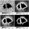 |
Fig. 5 Structure of magnetic field around the pore (in logarithmic scale) at 17:09 UT. The field of view is 20′′ × 16 |
The structure of the extended magnetic field was observed in the four best k–ω filtered images acquired at 17:09, 17:12, 17:22, and 17:33 UT. The first one is shown in Fig. 5. A logarithmic scale is used for visualisation to enhance the weak magnetic field; the pore’s area is masked. We can see from the images that B extends from the WL pore border by more than 35. The horizontal component is more extended than the vertical one; at distances > 17 from the border, Bz is small, lower than 250 G. Isolated enhancements in Bz are co-spatial with G-band bright points. However, these features are not frequent in the surroundings of this pore. The extended field has a radial filamentary structure (“spines”, cf. Lites et al. 1993). The spines in Bz are identical to those in Bhor and co-spatial with the dark intergranular lanes. In the granulation farther than 17 from the pore’s border, the observed field is mostly horizontal and concentrated in intergranular lanes. This field is expected to be an extension of the horizontal magnetic field at the periphery of the pore.
7. Line-of-sight and horizontal velocity fields
The most conspicuous features in the LOS velocity maps are two small-scale downflow patches that appear successively at the southern border of the large umbral core. One of them is seen as a bright feature in the vLOS map in Fig. 2. Each patch persists for 20 min, their effective diameters are 09 and 06, and their maximum LOS speeds are 1.3 and 1.2 km s-1, respectively. Similar downdrafts were observed by Hirzberger (2003). Other downflow areas with vLOS < 0.8 km s-1 are also mostly located near the southern border of the large core. We note that at this location, the magnetic field quickly decreases with distance from the pore’s edge (cf. Fig. 5).
The pore is surrounded by numerous divergence centres of horizontal motions formed by recurrently exploding granules (Sobotka et al. 1999; Vargas Domínguez et al. 2010). The nearest divergence centres form an intermittent ring-like structure (Fig. 2) at an average distance 18–19 from the pore’s border, which is comparable to the extension of the horizontal magnetic field Bhor ≃ B = 400 G, i.e., the equipartition field strength.
Although the horizontal motions derived from WL images by the LCT method may not represent the real plasma motions, we expect there to be a statistical relation between these motions and the LOS velocity field. From the continuity equation, it follows that upflows should appear in places with positive divergence of horizontal velocities, while downflows should be observed in areas with negative divergence (November 1989). Since  is set in the umbra, the convective blueshift of granules may introduce a bias of about − 200 m s-1 in the spatially averaged granular LOS velocity (Dravins et al. 1981).
We now attempt to find the relation between vLOS and the horizontal velocity vector vhor by comparing the vLOS maps with the vhor divergence maps. The FOV is separated into regions with a positive divergence of div vhor > 0.07 s-1 (prevailing horizontal outflows) and a negative divergence of div vhor < − 0.07 s-1 (prevailing horizontal inflows). The mean values of vLOS are calculated separately for magnetised granulation (400 < B < 1200 G) in the vicinity of the pore’s border and for non-magnetic granulation (B < 400 G) far from the pore. The individual scatter in vLOS is quite large (σvLOS ≃ 250 m s-1) owing to granular convection. In magnetised granulation, we can find an average downflow of 40 m s-1 in regions with inflows and an average upflow of − 140 m s-1 in regions with outflows. In this case, the influence of convective blueshift is small, because granules are smaller and intergranular lanes broader than in non-magnetic areas. In non-magnetic granulation, an average upflow of − 120 m s-1 in regions with inflows and a larger upflow of − 240 m s-1 in regions with outflows are found. These velocities are clearly biased by the convective blueshift, because downflow areas in intergranular lanes are much smaller than granules with upflows. Subtracting the convective blueshift of 200 m s-1 we obtain downflows in inflow areas and upflows in outflow ones. Owing to the uncertainty in the vLOS measurement (see Sect. 3), we do not attempt to discuss this result in a quantitative way.
8. Discussion and conclusions
On the basis of spectropolarimetric data of spatial resolution better than 04 and a Stokes profiles inversion, we have measured the vector magnetic field, LOS velocities, and horizontal flows in and around a large solar pore and analysed their mutual relations. The magnetic field with time-averaged maximum strength of 2000 G was, as a whole, inclined to the west by 10°, away from the rest of the active region.
Both the LOS and horizontal motions have been suppressed by the magnetic field inside the pore (cf. Sankarasubramanian & Rimmele 2003; Hirzberger 2003). The magnetic and velocity signatures of umbral dots are absent, because the Fe I 617.3 nm line is formed too high to detect them. Several small-scale regions with strong downflows are observed at the pore’s border. The strongest (maximum 1.3 km s-1) downflows persist for 20 min. This is consistent with the results reported by Hirzberger (2003).
The magnetic field extends from the WL pore border more than 35 and has a radial structure in the form of spines. This field extension around sunspots and pores was first reported by Keppens & Martínez Pillet (1996) and its spinal structure by Lites et al. (1993). The spines are co-spatial with dark intergranular lanes, which is consistent with the numerical simulations of Cameron et al. (2007). The horizontal component is more extended than the vertical one; at a distance of 17 from the border, Bz ≃ 250 G, while Bhor decreases to the same value at 36. In their Fig. 7, Cameron et al. (2007) showed that there are approximately equal rates of decrease for Bz and Bhor, which is inconsistent with our observations. However, the rates of decrease depend on the pore diameter, and the pore simulated by Cameron et al. (2007) was more than four times smaller than the pore we observed.
The most important results of the analysis of relations between magnetic and velocity fields in the pore and its vicinity (Sects. 5 and 7) can be summarised as follows:
The magnitude of the vertical component Bz controls the decrease in temperature. The temperature decreases with Bz practically linearly, by about − 300 K kG-1 in the photosphere, − 350 K kG-1 in light bridge, and − 800 K kG-1 in the umbra. The contrast of granulation temperature pattern, characterised by σT, increases with increasing magnetic field strength and the temperature pattern is then suppressed for Bz > 1200 G and Bhor > 1000 G. The values Bz = 1200 G and Bhor = 1000 G are typical of the pore boundary (cf. Sütterlin 1998).
Granular upflows dominate in regions with BLOS < 600–700 G. For stronger fields, no flows are observed except for isolated downflows at the pore’s border. The LOS velocity signature of granulation (σvLOS) decreases with increasing BLOS but owing to the disturbing effect of downflows at the pore’s border it is difficult to determine at which BLOS the granulation signature is suppressed. The dependence of vLOS on the horizontal magnetic field component is similar to that on the LOS component. The signature of granulation (σvLOS) decreases for Bhor > 400 G and is practically suppressed for Bhor > 1000 G.
In the light bridge, the character of LOS flows is opposite of that of the photosphere: downflows in weaker field (BLOS < 900 G) and weak upflows or zero for stronger BLOS. This may be specific to this particular LB, because downflows appear in the northern part of the LB, where B and BLOS are weaker.
The horizontal-velocity signature of granulation σvhor gradually weakens for Bz > 500 G. Apart from this finding, we have not found clear relations between LCT horizontal velocities and magnetic field components. The nearest divergence centres of horizontal motions, which were formed by exploding granules, form an intermittent ring-like structure around the pore (cf. Sobotka et al. 1999). The average distance of this “ring” is 18–19 from the pore’s border. In this region, Bhor ≃ B is comparable to the equipartition field strength 400 G.
In both magnetised and non-magnetic granulation, we have found that, after the correction for convective blueshift, areas of divergent horizontal motions of granules are statistically related to upflows, while areas of convergent motions are related to downflows. This confirms the results of November (1989) at the scale of local granular motions.
We can conclude from these findings that granular convection is suppressed in magnetic fields with Bz > 1200 G and Bhor > 1000 G (within the pore). Granular upflows at the formation height of the line Fe I 617.3 nm are reduced already at Bz > 600–700 G. From the increase in temperature contrast (σT) with B, we can deduce that granules in the extended magnetic field around the pore become smaller and intergranular lanes broader than in the non-magnetic regions. Horizontal motions in granulation start to be damped for Bz > 500 G and recurrently exploding granules (divergence centres) appear only in magnetic fields comparable to or weaker than the equipartition field strength 400 G. These conclusions, drawn from the observation of a single pore, should be verified on a larger statistical sample.
Acknowledgments
We express our thanks to an anonymous referee, whose remarks contributed to the improvement of the paper. We thank Marta Vantaggiato for her participation in the observations. This work was supported by grant IAA 300030808 of the Grant Agency of the Academy of Sciences of the Czech Republic. The Dunn Solar Telescope is located at the National Solar Observatory, which is operated by the Association of Universities for Research in Astronomy, Inc. (AURA), for the National Science Foundation. IBIS has been built by INAF/Osservatorio Astrofisico di Arcetri with contributions from the Universities of Firenze and Roma “Tor Vergata”, the National Solar Observatory, and the Italian Ministries of Research (MIUR) and Foreign Affairs (MAE).
References
- Cabrera Solana, D., Bellot Rubio, L. R., & del Toro Iniesta, J. C. 2005, A&A, 439, 687 [NASA ADS] [CrossRef] [EDP Sciences] [Google Scholar]
- Cameron, R., Schüssler, M., Vögler, A., & Zakharov, V. 2007, A&A, 474, 261 [NASA ADS] [CrossRef] [EDP Sciences] [Google Scholar]
- Cavallini, F. 2006, Sol. Phys., 236, 415 [NASA ADS] [CrossRef] [Google Scholar]
- Choudhuri, A. R. 1986, ApJ, 302, 809 [NASA ADS] [CrossRef] [Google Scholar]
- del Toro Iniesta, J. C. 2003, Introduction to Spectropolarimetry, Sect. 11.2.1 (Cambridge: Cambridge University Press) [Google Scholar]
- Dravins, D., Lindegren, L., & Nordlund, Å. 1981, A&A, 96, 345 [NASA ADS] [Google Scholar]
- Fried, D. 1982, J. Opt. Soc. Am., 72, 52 [Google Scholar]
- Giordano, S., Berrilli, F., Del Moro, D., & Penza, V. 2008, A&A, 489, 747 [NASA ADS] [CrossRef] [EDP Sciences] [Google Scholar]
- Hirzberger, J. 2003, A&A, 405, 331 [NASA ADS] [CrossRef] [EDP Sciences] [Google Scholar]
- Hulburt, N. E., & Rucklidge, A. M. 2000, MNRAS, 314, 793 [Google Scholar]
- Jurčák, J. 2011, A&A, 531, A118 [NASA ADS] [CrossRef] [EDP Sciences] [Google Scholar]
- Keil, S. L., Balasubramaniam, K. S., Smaldone, L. A., & Reger, B. 1999, ApJ, 510, 422 [NASA ADS] [CrossRef] [Google Scholar]
- Keppens, R., & Martínez Pillet, V. 1996, A&A, 316, 229 [NASA ADS] [Google Scholar]
- Landi Degl’Innocenti, E. 1982, Sol. Phys., 77, 285 [NASA ADS] [CrossRef] [Google Scholar]
- Lites, B. W., Elmore, D. F., Seagraves, P., & Skumanich, A. P. 1993, ApJ, 418, 928 [NASA ADS] [CrossRef] [Google Scholar]
- Lites, B. W., Low, B. C., Martínez Pillet, V., et al. 1995, ApJ, 446, 877 [NASA ADS] [CrossRef] [Google Scholar]
- Neckel, H. 1999, Sol. Phys., 184, 421 [NASA ADS] [CrossRef] [Google Scholar]
- Norton, A. A., Graham, Graham, J. P., Ulrich, R. K., et al. 2006, Sol. Phys., 239, 69 [Google Scholar]
- November, L. J. 1989, ApJ, 344, 494 [NASA ADS] [CrossRef] [Google Scholar]
- November, L. J., & Simon, G. W. 1988, ApJ, 333, 427 [Google Scholar]
- Ortiz, A., Bellot Rubio, L. R., & Rouppe van der Voort, L. 2010, ApJ, 713, 1282 [NASA ADS] [CrossRef] [Google Scholar]
- Parker, E. N. 1979, ApJ, 234, 333 [NASA ADS] [CrossRef] [Google Scholar]
- Rimmele, T. R., Richards, K., Hegwer, S., et al. 2009, in Telescopes and Instrumentation for Solar Astrophysics, ed. S. Fineschi, & M. A. Gummin, Proc. SPIE, 5171, 179 [Google Scholar]
- Rucklidge, A. M., Schmidt, H. U., & Weiss, N. O. 1995, MNRAS, 273, 491 [NASA ADS] [CrossRef] [Google Scholar]
- Ruiz Cobo, B., & del Toro Iniesta, J. C. 1992, ApJ, 398, 375 [NASA ADS] [CrossRef] [Google Scholar]
- Sankarasubramanian, K., & Rimmele, T. 2003, ApJ, 598, 689 [NASA ADS] [CrossRef] [Google Scholar]
- Scharmer, G. B., Henriques, V. M. J., Kiselman, D., & de la Cruz Rodríguez, J. 2011, Science, 333, 316 [NASA ADS] [CrossRef] [Google Scholar]
- Simon, G. W., & Weiss, N. O. 1970, Sol. Phys., 13, 85 [NASA ADS] [CrossRef] [Google Scholar]
- Simon, G. W., Title, A. M., Topka, K. P., et al. 1988, ApJ, 327, 964 [NASA ADS] [CrossRef] [Google Scholar]
- Sobotka, M. 2003, Astron. Nachr., 324, 369 [NASA ADS] [CrossRef] [Google Scholar]
- Sobotka, M., & Jurčák, J. 2009, ApJ, 694, 1080 [NASA ADS] [CrossRef] [Google Scholar]
- Sobotka, M., Vázquez, M., Bonet, J. A., Hanslmeier, A., & Hirzberger, J. 1999, ApJ, 511, 436 [NASA ADS] [CrossRef] [Google Scholar]
- Solanki, S. K., & Stenflo, J. O. 1985, A&A, 148, 123 [NASA ADS] [Google Scholar]
- Stix, M. 1989, The Sun, 1st edition (Berlin: Springer) [Google Scholar]
- Sütterlin, P. 1998, A&A, 333, 305 [NASA ADS] [Google Scholar]
- Sütterlin, P., Schröter, E. H., & Muglach, K. 1996, Sol. Phys., 164, 311 [NASA ADS] [CrossRef] [Google Scholar]
- Thomas, J. H., & Weiss, N. O. 2004, ARA&A, 42, 517 [NASA ADS] [CrossRef] [Google Scholar]
- van Noort, M., Rouppe van der Voort, L., & Löfdahl, M. 2006, in Solar MHD Theory and Observations, ed. J. Leibacher, R. F. Stein, & H. Uitenbroek, ASP Conf. Ser., 354, 55 [Google Scholar]
- Vargas Domínguez, S., de Vicente, A., Bonet, J. A., & Martínez Pillet, V. 2010, A&A, 516, A91 [NASA ADS] [CrossRef] [EDP Sciences] [Google Scholar]
- Viticchié, B., Del Moro, D., Criscuoli, S., & Berrilli, F. 2010 ApJ, 723, 787 [Google Scholar]
- Wedemeyer-Böhm, S. 2008, A&A, 487, 399 [NASA ADS] [CrossRef] [EDP Sciences] [Google Scholar]
All Tables
All Figures
|
Fig. 1 Pore in NOAA 11005 observed on 15 October 2008 at 17:14 UT. Left – white-light image, right – Ca II 854.2 nm line-centre image. The field of view is 39′′ × 39′′, centred at the position 25.2 N 10.0 W; a black arrow indicates the direction to the disc centre. Symbols “+” and “ × ” mark the positions of the maximum magnetic field strength and its horizontal component, respectively. |
| In the text | |
|
Fig. 2 Time-averaged grey-scale maps of physical parameters obtained for the period 17:09–17:18 UT. The field of view is 20′′ × 16 |
| In the text | |
|
Fig. 3 Map of LCT horizontal velocities for the period 17:09–17:18 UT. We have superimposed the white-light image. The length of the black horizontal bar at the bottom left corner represents 1 km s-1. |
| In the text | |
|
Fig. 4 Graphs of relations between temperature T, LOS velocity vLOS, horizontal velocity vhor and magnetic field components BLOS, Bz, and Bhor. Left – mean values, right – σ values. Black line – photospheric granulation, red (thick) – light bridge, green (grey) – umbra. |
| In the text | |
|
Fig. 5 Structure of magnetic field around the pore (in logarithmic scale) at 17:09 UT. The field of view is 20′′ × 16 |
| In the text | |
Current usage metrics show cumulative count of Article Views (full-text article views including HTML views, PDF and ePub downloads, according to the available data) and Abstracts Views on Vision4Press platform.
Data correspond to usage on the plateform after 2015. The current usage metrics is available 48-96 hours after online publication and is updated daily on week days.
Initial download of the metrics may take a while.