| Issue |
A&A
Volume 537, January 2012
|
|
|---|---|---|
| Article Number | A150 | |
| Number of page(s) | 11 | |
| Section | The Sun | |
| DOI | https://doi.org/10.1051/0004-6361/201117580 | |
| Published online | 25 January 2012 | |
Solar low-lying cool loops and their contribution to the transition region EUV output
1 INAF-Osservatorio Astronomico di Capodimonte, Salita Moiariello 16, 80131 Napoli, Italy
e-mail: csasso@oacn.inaf.it
2 INAF-Osservatorio Astrofisico di Catania, via S. Sofia 78, 95123 Catania, Italy
Received: 28 June 2011
Accepted: 25 November 2011
Aims. We aim to investigate the increase of the differential emission measure (DEM) towards the chromosphere. In the past 30 years, small and cool magnetic loops (height ≲ 8 Mm, T ≲ 105 K) have been proposed as an explanation for this effect.
Methods. We present hydrodynamic simulations of low-lying cool loops in which we studied the loops’ conditions of existence and stability, and their contribution to the transition region EUV output.
Results. We find that stable, quasi-static cool loops (with velocities <1 km s-1) can be obtained under different and more realistic assumptions on the radiative loss function with respect to previous works. A mixture of the DEMs of these cool loops plus intermediate loops with temperatures between 105 and 106 K can reproduce the observed emission of the lower transition region at the critical turn-up temperature point (T ~ 2 × 10⁵ K) and below T = 105 K.
Key words: Sun: transition region / Sun: UV radiation / hydrodynamics
© ESO, 2012
1. Introduction
In the past 30 years, different theories have been proposed and debated to explain the origin of the solar EUV output at temperatures below 1 MK. The idea that the transition region (hereafter TR) emission originates from the bases of the hot large-scale coronal loops is not confirmed by the measured differential emission measure (DEM), which is orders of magnitude higher than predicted (Gabriel 1976; Athay 1981). The observed excess emission compared to the predictions of the traditional conduction-dominated TR picture has led, in particular, to the suggestion that much of the TR plasma is confined in relatively small and cool magnetic loops (height ≲ 8 Mm, T ≲ 105 K) that are strongly connected to the chromosphere, but are thermally insulated from the corona (Dowdy et al. 1986; Dowdy 1993; Feldman 1983; Feldman et al. 2001).
The existence of this class of magnetic loops, predicted for decades, remains far from being established. From the observational point of view, they are indeed very difficult to observe. Because most of their emission is in the UV, traditional chromospheric diagnostics from the ground, such as H α, only carry information about their lower boundary. On the other hand, the lack of spectral information with proper temperature sensitivity and spatial resolution from the current space-born EUV instruments that are capable of observing lines forming between 104 and 105 K has so far prevented any firm conclusions.
Some recent observations with the VAULT instrument (Very High Angular Ultraviolet Telescope, Korendyke et al. 2001) in the H i Ly-α line at very high spatial resolution showed loop-like structures with estimated temperatures and densities (T = 104−3 × 10⁴ K, P = 0.1−0.3 dyne cm-2) that could be appropriate for the low-temperature end of cool loops (Patsourakos et al. 2007; Vourlidas et al. 2010). While this interpretation has been debated (Judge & Centeno 2008), those observations, together with the persistence of the problem of the excess emission in EUV lines below 105 K, call for additional investigations on the matter.
The general properties of static cool loops were first discussed by Hood & Priest (1979) and then studied more in detail from a theoretical point of view by Antiochos & Noci (1986), who demonstrated analytically that a mixture of static cool loops with different temperatures can account for the observed lower transition region DEM. This class of loops has specific characteristics compared to the better studied coronal loops. While large-scale hot coronal loops have dimensions of the order of ~10 Mm, temperatures higher than 106 K, and obey the “static” scaling laws described by Rosner et al. (1978, hereafter RTV), cool loops are low-lying (estimated heights of the order of 1.1–5 Mm), nearly isobaric, and have a maximum temperature of below 105 K. Another major difference with respect to classical coronal loops is the role played by the three terms appearing in the hydrodynamical equation of plasma energy conservation: the heating rate, the conductive flux, and the radiative losses. Static cool loops are in approximate balance between the heating rate and radiative losses. Therefore, in contrast to coronal loops, the conductive flux plays a negligible role.
Cally & Robb (1991), following the study of Antiochos & Noci (1986), treated the stability, structure, and evolution of these static cool loops in more detail, both analytically and numerically. They revealed, in particular, that the shape of the radiative loss function, Λ(T), poses restrictive conditions on the existence of static cool loops. For a realistic radiative loss function with an H i Ly-α loss peak around T = 2 × 10⁴ K (e.g., Dere et al. 2009; or Colgan et al. 2008, dotted and long-dashed line in Fig. 1, respectively), strictly static cool loops do not exist (see the next sections for details). It is important to note that the analysis of Cally & Robb (1991) was limited to a minimum temperature of log T = 4.29 K, so that they could not consider loops with a maximum temperature below this value and could not include Ly-α losses properly (even in the thin losses case). They obtained static cool loops numerically with a maximum temperature of around T = 8 × 10⁴ K, assuming a T3 dependence of the radiative loss function on the temperature below T = 105 K (dashed line in Fig. 1). They concluded, however, that this temperature is a factor 2–3 too low to explain the observed low-TR emission, although they did not show any calculated DEM function to support these conclusions. Moreover, they stated that “the steep T3 radiative loss function even if so beneficial for the existence and stability of cool loops rests on shaky foundations”.
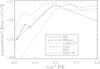 |
Fig. 1 Radiative loss functions considered in this work. Solid line: power-law segments function, equal to T2 (for log T < 4.95 K) and T-1 (for log T > 4.95 K); solid line plus star symbols: a peak mimicking the H Ly-α losses was added to the previous function; dashed line: from Cook et al. (1989), but with a T3 dependence below T = 105 K; long-dashed line: from Colgan et al. (2008); dotted line: from Dere et al. (2009); dot-dashed line: from Dere et al. (2009) without the H contribution. |
After the cited work of Cally & Robb (1991), our paper is the first attempt to study the conditions of existence of small and cool loops (height ≲ 5 Mm, T ≲ 105 K) numerically and, if they do exist, their physical structure and their contribution to the TR emission. We show that stable, quasi-static cool loops (with plasma velocities < 1 km s-1) can be obtained through hydrodynamic simulations also assuming different forms of Λ(T), than Cally & Robb (1991).
Peter et al. (2004, 2006) made the first successful attempt to reproduce the shape of the DEM curve quantitatively and qualitatively, even at temperatures below log T = 5.3 K. They used a forward model in which they synthesized spectra from three-dimensional MHD simulations of the whole Sun atmosphere, from the chromosphere to the corona. Our results are not mutually exclusive. Their simulations include structures that could be related to the kind of loops we are studying. However, the loops we describe in this paper would be covered by only very few resolution elements in their simulation, and in any case resolving the gradients and the dynamics of the relevant quantities in our loop models would require a much higher resolution. Therefore, we regard our study as complementary to the kind of large-scale simulations by Peter et al. (2006).
In the course of our study of loops with the properties just described, we have also found low-lying quasi-static loops with temperatures in the range 105 − 106 K. Following one of the latest loop classifications (Reale 2010), we should refer to these loops also as “cool loops”. In order to avoid confusion, we will refer to them as “intermediate-temperature loops”. This class of loops was first studied by Foukal (1976) and observed by Brekke et al. (1997). From observations, they are generally detected in the UV lines and appear to be steady for long times even if they are more variable and dynamic than hot coronal loops, probably because of substantial flows (Brekke et al. 1997; Di Giorgio et al. 2003; Reale 2010). Their estimated densities are in the range 109−1010 cm-3 (e.g., Brown 1996). Although observed intermediate-temperature loops are often related to flows, we decided to report in this paper our findings on their existence (at least analytically) in a quasi-static state. Studying the role of flows for the conditions of their existence would mean introducing a new dimension in the parameter space to be explored, and this is beyond the scope of this paper, which concentrates on quasi-static cool loops. The quasi-static intermediate-temperature loops we find have different physical properties compared to observed loops with that temperature and this may be correlated with flows.
The paper is structured as follows: in Sect. 2, we describe the numerical model, and introduce the different radiative loss functions adopted. In Sect. 3, we present the hydrodynamic simulations and the different loops obtained (cool and intermediate-temperature loops) and we discuss and analyze their properties. Section 3.3 is dedicated to the calculated DEMs of these loops and to the comparison with the observed one. Finally, in the conclusions (Sect. 4), the role of the cool and intermediate-temperature loops in the solar atmosphere and the possibility to observe them with current instrumentation is treated.
2. Numerical modelling and calculations
The set of hydrodynamic equations for mass, momentum, and plasma energy conservation for a fully ionized hydrogen plasma have been solved in an unidimensional, magnetically confined loop of constant cross-section with ARGOS, a 1-D hydrodynamic code with the fully adaptive-grid package PARAMESH (Antiochos et al. 1999; MacNeice et al. 2000). A fully adaptive-grid is necessary to adequately resolve one or more evolving regions of steep gradients, for example the thin segments of the transition region chromosphere-corona of the loop (for coronal loops) or shocks in dynamical simulations. The geometry of the loop is determined by the following analytic form: 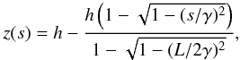 (1)where z is the height above the chromospheric footpoints, s is the curvilinear coordinate along the field lines, h is the height of the loop apex (i.e., zmax), L is the loop total length, and the constant γ is defined in terms of h and L as
 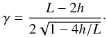 (2)This form implies that z(s) = 0 at the footpoints, z(s) has its maximum h at the midpoint, s = 0, and dz/ds = ± 1 when s = ± L/2. Equations (1) and (2) generate an arched loop of a given length L and apex height above the chromosphere h.
The numerical model includes a thick chromosphere at each footpoint 26.7 Mm deep, acting as a mass reservoir; the total length of the flux tube is therefore L + 53.4 Mm. The boundary conditions imposed are at the two endpoints (rigid wall, fixed temperature), which are located at s = ± (L/2 + 26.7) Mm. The temperature of this chromosphere is set at T = 104 K. This is new with respect to previous works, in which the chromospheric temperature was set to T = 2 or 3 × 10⁴ K (e.g. Antiochos & Noci 1986; Cally & Robb 1991; Spadaro et al. 2003). A chromospheric temperature at 104 K allows the inclusion of the full peak of the H i Ly-α line in the optically thin radiative loss function and to explore the temperature range (104−3 × 10⁴ K) observed by VAULT. The inclusion of the Ly-α as an optically thin line is of course only a first step, suitable for this exploratory study. Work is in progress to take into account the transfer of Ly-α radiation, and to include partial plasma ionization at the lower temperature end of the simulations. Since we take, by definition, the beginning of the chromosphere as the level at which the plasma drops below 104 K, the exact position of the top of the chromosphere (s = ± Li/2 at the beginning of the simulation) changes during the calculation with the plasma filling or evacuating the loop. So, at end of the simulation, we will have a new position for the top of the chromosphere s = ± Lf/2 and, consequently, a new value of h = hf, where hf is no longer the geometrical parameter defining the shape of the loop, but the height of the loop apex above the T = 104 K level.
The set of conservation equations for mass, momentum, and energy in a one-dimensional plasma solved by ARGOS is 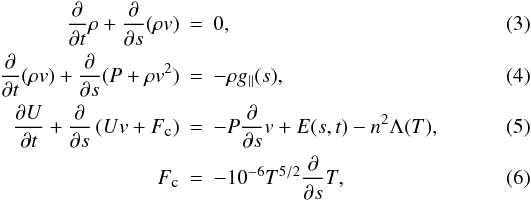 where t is the time, ρ the mass density, v the velocity, P, T and n are the gas pressure, temperature, and electron number density, respectively, linked by the equation of state P = 2nkT, with k the Boltzmann constant; U = 3P/2 is the internal energy, s the curvilinear coordinate along the loop, E(s,t) the assumed form for the coronal heating rate, n2Λ(T) the plasma optically thin radiative losses, with Λ(T) the radiative loss function, g ∥ (s) the component of the solar gravity along the loop axis, and Fc the thermal conductive flux, in CGS units.
2.1. Radiative loss functions
The hydrodynamic simulations were performed assuming different shapes for the radiative loss function, which are shown in Fig. 1. Since radiative losses were hard-coded in the original version of ARGOS, we modified the code to allow for arbitrary, tabulated Λ(T). We verified with some benchmark tests that the modification does not introduce significant overheads in the calculations. First, we use the same approximation of the radiative loss function as adopted by Antiochos & Noci (1986, solid line in Fig. 1, ΛAN in Table 1, who fitted the data of Gaetz & Salpeter (1983), assuming that the Λ(T) can be approximated by an increasing power-law of temperature for log T < 4.95 K ( ∝ Ta), and by a decreasing power-law for log T > 4.95 K ( ∝ T − b), with a and b both positive. In particular: 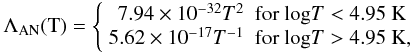 (7)this approximation does not consider the peak caused by the H Ly-α radiative losses at around T = 2 × 10⁴ K. In order to study its effect on the simulations, we added to the function ΛAN a peak mimicking the H Ly-α losses (solid line plus cross symbols in Fig. 1, ΛANLyα in Table 1). The peak has approximately the same shape of the one in the realistic radiative loss function ΛCea that we are going to describe. It was built by taking the two lines parallel to the ascending and to the descending branches of the Ly-α peak present in the function ΛCea, and making them pass through the point with abscissa log T = 4.21 K, corresponding to the peak top value.
The long-dashed line and the dotted line in Fig. 1 are two realistic radiative loss functions. The first is from the work of Colgan et al. (2008, ΛCea in Table 1 and the other was obtained using the “CHIANTI” database, version 6 (Dere et al. 2009, ΛDea in Table 1), adopting the ionization equilibrium of Bryans et al. (2009), and a coronal mixture of elements. We chose these two functions because they are the most recent and are based on the latest atomic data available. A discussion on the differences, quite significant, between the two functions can be found in Dere et al. (2009).
The last radiative loss function used in this paper has been obtained by removing the contribution of hydrogen from the function ΛDea (dot-dashed line Fig. 1, ΛDea − H in Table 1). Even after subtracting the hydrogen losses, a smaller peak remains at around T = 2 × 10⁴ K owing to other elements losses (mainly helium).
In the next section, we introduce the results from simulations using these different radiative loss functions. The list of simulated loops, together with the relevant parameters, is given in Table 1.
Loop parameters.
3. Results and discussion
To derive the initial equilibrium, we followed the approach of Spadaro et al. (2003), i.e., we simply started with a discontinuous temperature profile in which T = Ti (with Ti a constant value) in the corona and T = 104 K in the chromosphere. The density was constant in the corona, n = ni, and increased exponentially with depth in the chromosphere at the appropriate scale height. Hence, the plasma was in approximate force balance to start with, but not in thermal equilibrium. During the simulation, the loop evolves towards a stable quasi-static solution of the hydrodynamic equations (Eqs. (3)–(5)), a solution, that is, which approximately fulfills the static and stationary versions of these equations: 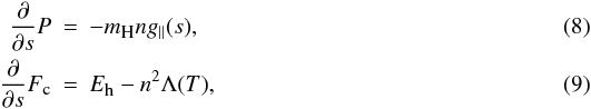 where we used ρ = mHn for a fully ionized hydrogen plasma with mH the hydrogen mass. We consider a loop in a quasi-static equilibrium state when the plasma velocities are lower than 1–2 km s-1. With this definition, we find that in all our simulations the thermodynamic parameters of a loop in quasi-static equilibrium oscillate around the equilibrium value with an amplitude much smaller than 1%. We took this quasi-static equilibrium state as a result or, in some cases (see below), as an initial equilibrium state (t = 0 s) for a new simulation with different parameters (e.g.: different heating rate).
In all simulations we assumed a spatially uniform and temporally constant heating rate per unit volume, E(s,t) = Eh, and we ensured that they last long enough for the end time to be much longer than the loop radiative cooling time.
3.1. Description of results
We ran numerous simulations, extensively exploring the parameter space, under different initial conditions. We list in Table 1 and discuss below a representative selection of the loops in quasi-static equilibrium that we obtained. Loops 3–4, 7–13, and 17–23 are obtained by starting the simulation with a loop in approximate force balance but not in thermal equilibrium as described previously, using different combinations of Ti and ni that we thought be appropriate for cool loops. All these simulations have an initial half length, Li/2 = 6.5 Mm and an initial height, hi = 0.62 Mm. Once we obtained two quasi-static cool loops (loops 3 and 4), we used them as initial equilibrium states to perform new simulations. In this way, starting in particular from loop 3 and changing some parameters, we obtained all other cool loops 1–2, 5–6, 14–16, and 24–26. Loops 1 and 2 were obtained by changing the heating rate and the initial height, hi = 0.7 Mm. Loops 5 and 6 were obtained by changing the heating rate and the initial height again, but to the value hi = 0.54 Mm. Finally, loops 14–16 and 24–26 have again different heating rates but also different radiative loss functions.
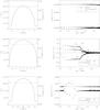 |
Fig. 2 Top panel, left: temperature (solid line) and pressure (dashed line) as a function of the curvilinear coordinate along the field lines, s. Right: divergence of the conductive flux (asterisks), radiative losses (crosses) and constant heating rate, Eh (solid line), as a function of the temperature, for loop 4. Middle and bottom panels: as in the top panels for loop 10 and 15, respectively. |
3.1.1. Loops from idealized Λ(T)
The first group of simulations we made assumes as a radiative loss function ΛAN, in order to test the analytical results of Antiochos & Noci (1986). We were able to obtain quasi-static cool loops with maximum temperature between ~2.6 and 8.3 × 10⁴ K, using Eh in the range 4−7.5 × 10⁻⁴ erg cm-3 s-1. In Table 1 we report only some examples of the cool loops found (loops 1–6). These loops have the properties analytically predicted by Antiochos & Noci (1986): they are small (L/2 = 0.7−2.5 Mm and h = 0.005−0.04 Mm), nearly isobaric, and in approximate balance between the heating rate and radiative losses, Eh = n2Λ(T) ≫ |∇Fc|. The low-pressure values compared to coronal hot loops were also analytically predicted by Antiochos & Noci (1986). According to their calculations, the pressure of a cool loop has to be at least one and one-half order of magnitude lower than that of a hot loop with maximum temperature higher than 106 K. This result is confirmed by our calculations.
In Figs. 2 and 3 we plot the behaviour of the loop parameters as well as of the terms of the energy Eq. (9) for five loops chosen as examples for each group of loops obtained with a different Λ(T) (loops 4, 10, and 15 from top to bottom in Fig. 2, and loops 17 and 25, from top to bottom in Fig. 3). The left panels show the temperature (solid line) and the pressure (dashed line) profiles as a function of the curvilinear coordinate, s, while the right panels show the radiative losses energy term, n2Λ(T) (crosses), the heating rate, Eh (solid line), and the divergence of the conductive flux, ∇Fc (asterisks), as a function of the temperature. The plots show the variation of loop temperature, density, and energy terms along the loop at a particular instant (corresponding to the end time of the simulation). Since the loops are still in a quasi-static equilibrium state, with the plasma subject to motions (oscillations, for instance) of small, but not negligible amplitude, those profiles do not appear exactly symmetric around the loop apex (s = 0). Averaging profiles over an appropriate number of time steps would cancel out these small variations, thus yielding nearly symmetric profiles.
The maximum temperature of loop 4 (top left panel of Fig. 2), chosen as the example for the first group of loops 1–6, is 8.3 × 10⁴ K and the pressure is constant along the loop (within 1% above the chromosphere). The terms n2Λ(T) and Eh are in approximate balance, while the divergence of the conductive flux is only a small term (right panel).
Using the same radiative loss function, we also obtained quasi-static intermediate-temperature loops with maximum temperature T ~ 8 × 10⁵ K (loops 7–13 in Table 1). For loop 10, we show in the middle panels of Fig. 2 the behaviour of the temperature and the pressure as a function of s (left) and of the terms of the energy equation as a function of the temperature (right). The two terms competing in the energy balance are the divergence of the conductive flux (asterisks) and the radiative losses term (crosses) as in hot coronal loops.
We explored the possibility of obtaining stable cool loops also with the function ΛANLyα. Using the cool loop 3 of Table 1 as a starting solution, we made a simulation by changing the radiative loss function from ΛAN to ΛANLyα. The temperature of loop 3 drops below T = 2 × 10⁴ K (the position of the Ly-α peak) and a quasi-static, stable, cool loop of maximum temperature 1.2 × 10⁴ K forms (loop 14 in Table 1). The temperature of this loop is comparable with the loop-like structures observed by VAULT but the pressure is ten times lower. Loop 14 is also lower and shorter compared to loop 3. In order to obtain hotter loops (but still cool, with T < 105 K) from loop 3 by changing only Eh and using ΛANLyα, we have to raise its value from 5.5 × 10⁻⁴ erg cm-3 s-1 to 5.8 × 10⁻⁴ erg cm-3 s-1. The increase of Eh should compensate for the higher radiative losses (because of the introduction of the Ly-α peak) and allow the loop to keep the initial equilibrium without dropping to low temperatures. We indeed obtained a quasi-static cool loop with maximum temperature T = 7.4 × 10⁴ K (loop 15 in Table 1). Loop 16 of Table 1 is instead obtained with Eh = 5.9 × 10⁻⁴ erg cm-3 s-1 and ΛANLyα. Using Eh = 6 × 10⁻⁴ erg cm-3 s-1, the loop reaches a maximum temperature much higher than 105 K. So, loop 15 and 16 are the two loops with temperatures higher than the temperature of the Ly-α peak that can be obtained from loop 3 changing only Eh and the radiative loss function to ΛANLyα. We are then able to “overcome” the Ly-α peak, whose presence was thought to prevent the existence of cool loops (Cally & Robb 1991). The three cool loops 14–16 have the same characteristics already described for loops 1–6. In the bottom panels of Fig. 2, we show the behaviour of the temperature and the pressure as a function of s (left) and of the terms of the energy equation as a function of the temperature (right) for loop 15. The temperature of the loop starts to increase at around s = −1.1 Mm up to s ~ −1 Mm, reaching the value of ~1.2 × 10⁴ K and then increases rapidly till the maximum value of ~7.4 × 10⁴ K. Loop 16 has the same behaviour. The values of L/2 in Table 1 for these two loops include the piece where the temperature rises slowly. The terms competing in the energy balance are the radiative losses term (crosses) and the background heating (solid line) as for loops 1–6.
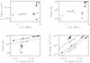 |
Fig. 4 Behaviour of the physical parameters for loops 1–6 (diamonds), 7–13 (crosses), 14–16 (triangles), 17–23 (asterisks) and 24–26 (squares) of Table 1. The solid lines represent the RTV scaling laws for coronal loops for different values of L/2. The dotted line represents Eh = P2. |
The intermediate-temperature loops we found are longer than cool loops. Because the loop height is linked to the loop length, lower loops are also shorter. In the next sections, we show that quasi-static cool loops need to be low-lying to satisfy the quasi-static equations with a negligible conductive flux. Intermediate-temperature loops, instead, do not need to be as short as cool loops because their length is linked to the pressure and to the heating rate by RTV-like scaling laws.
3.1.2. Loops from realistic, optically thin Λ(T)
Using the function of radiative losses ΛCea, we obtained only quasi-static loops with a peak temperature higher than 105 K (loops 18–23 in Table 1). Loop 17 was obtained with the realistic radiative loss function ΛDea but has the same properties as loop 18. For loop 17, we show in Fig. 3 the behaviour of the temperature and the pressure as a function of s (left panel) and of the terms of the energy equation as a function of the temperature (right panel). The energy balance terms behave as for intermediate-temperature loops 7–13.
Using ΛDea − H and following the same method as for ΛANLyα, we obtained the cool loops 24–26 of Table 1. The maximum temperature of loop 24 is lower than the temperature at which ΛDea − H shows the small peak (at T ~ 2 × 10⁴ K) that remains even if the hydrogen losses have been subtracted. Loops 25 and 26 have instead a higher temperature. For loop 25, in the bottom panels of Fig. 3 we show the behaviour of the temperature and the pressure as a function of s (left panel) and of the terms of the energy equation as a function of the temperature (right panel). As for loops 15 and 16, the temperature of loop 25 starts to increase at around s = −5.3 Mm up to s ~ −0.8 Mm, reaching the value of ~1.2 × 10⁴ K and then increases quickly till the maximum value of ~4 × 10⁴ K. Loop 26 follows the same behaviour. These two loops are longer compared to loops 15 and 16 if we consider the piece where the temperature rises slowly. We think that this difference is caused by the different slopes of the Λ(T) used in the two cases for T < 1.2 × 10⁴ K. So, considering a total height of 0.29 Mm for loop 25, only the top part with length of ~0.005 Mm is hot. This loop is really at the limit because of its dimensions and its shape may depend from the details of the boundary conditions and the radiative transfer as we suggested previously (the shape of Λ(T) around T = 104 K). In order to observe these types of loops, we would need at least two different spectral lines formed at temperatures between 104 and 2 × 10⁴ K to resolve the loop in its temperature extension and a very high resolution. As predicted by Antiochos & Noci (1986), also for loops 24–26, the terms competing in the energy balance are only the radiative losses term (crosses) and the background heating (solid line).
3.1.3. Relations between loop parameters and scaling laws
In Fig. 4 we show the relations between the thermodynamic parameters (P, Tmax and L/2) and the heating rate for the loops in Table 1 (loops 1–6 are represented by diamonds, loops 7–13 by crosses, loops 14–16 by triangles, loops 17–23 by asterisks, and loops 24–26 by squares). The solid lines in the lower panels of Fig. 4 represent the RTV scaling laws for coronal loops for different values of L/2, while the dotted line (lower-right panel) represents the law Eh = P2. The pressure of all cool loops with T < 105 K is proportional to the square root of Eh and it is independent of their length and maximum temperature. Intermediate-temperature loops 7–13 and 17–23 (with different proportional coefficients) obey the RTV scaling laws for coronal loops. This is a somewhat surprising result because their temperatures are lower than 106 K and observed intermediate-temperature loops do not obey the coronal scaling laws (Brown 1996). The model used by Rosner et al. (1978) to derive the relationships between coronal temperature, pressure, length and heating in coronal loops assumes a global energy balance between the heating and the radiative losses in static conditions. The majority of observed intermediate-temperature loops reveal temperatures and densities that lie outside the static model tracks and, as different authors have shown (e.g., Dere 1982; Durrant & Brown 1989), the static model does not seem to accurately predict their physical conditions. The difference between our loops and the observed ones is in the pressure. We obtained intermediate-temperature loops with pressures that are 1–2 orders of magnitudes lower than measured in observed loops with the same temperatures (Brown 1996). Loops 7–13 and 17–23 have the right pressures to fall on the scaling laws lines.
3.2. The conditions for the existence of cool loops
The quasi-static, stable cool loops with the characteristics predicted by Antiochos & Noci (1986) found are unexpected according to the considerations of Cally & Robb (1991). Assuming a form of Eh ∝ (n/n0)ν, with n0 the density at the loop base, the conditions of existence and stability of cool loops derived in the mentioned paper are not valid for ν = 0 (constant heating per unit volume) combined with a = 2. This combination should not allow strictly static solutions. So, it is quite remarkable that we obtained quasi-static cool loops with the radiative loss functions ΛAN, ΛANLyα, and ΛDea − H. The first two functions are, indeed, built with a T2 dependence below 105 K (excluding the peak for ΛANLyα) and, from Fig. 1, it is clear that ΛDea − H also follows the same behaviour (excluding the small peak).
a = 2 is also empirically a better approximation to realistic Λ(T) than a = 3 used by Cally & Robb (1991). They show that if the hydrogen losses are ignored, following the suggestion of McClymont & Canfield (1983) to obtain a better approximation to the true radiative loss function, cool loops can exist. They assume, however, that when ignoring the hydrogen losses the peak in the radiative loss function is replaced by a steep slope T3 for T < 105 K. Ignoring the contribution of hydrogen in the function ΛDea, for example, we obtain a dependence closer to T2. Looking also at the functions ΛDea e ΛCea it is possible to say that the approximation T2 below 105 K is closer to the shapes of realistic radiative loss functions than T3, and it is also often used (see, e.g.: Rosner et al. 1978; Antiochos & Noci 1986).
More surprising is the existence of cool loops even if the radiative loss function includes a peak around T = 2 × 10⁴ K. For Cally & Robb (1991), its presence prevents the existence of cool loops at the conditions we are considering (ν = 0) and not only. Their hydrodynamical simulations start always from an initial uniform cool state (log T = 4.3 K), corresponding to the equilibrium solution in the absence of gravity and, they say, the presence of the Ly-α plateau (they do not include the whole peak) prevents cool solutions, even unstable ones, with the loops reaching the hot state directly. All simulations performed with a radiative loss function including the Ly-α peak (ΛANLyα and ΛDea − H), start by setting the quasi-static cool loop 3 as initial equilibrium state (as described in Sect. 3.1) so that we did not have the problems faced by Cally & Robb (1991).
Moreover, the cool solutions we found not only exist, but are also stable (in contrast to previous predictions, e.g., Judge & Centeno 2008), in the sense that the loop thermodynamic properties oscillate around an average value. These oscillations are of small amplitude and do not grow with time. Occasionally, however, these oscillations bring the loop to a different stable state, determined by the particular shape of the Λ(T) adopted. The stability of these loops is therefore related to the chosen shape of Λ(T) and, in particular, to the temperature value at which it reaches its maximum or changes slope. For ΛAN, if we change the maximum temperature value to a higher one (and increase the value of Eh), we can still obtain stable cool loops with a higher maximum temperature. As an example, we have included in Table 1 loop 27 obtained by raising the temperature value at which ΛAN peaks from T = 104.95 to 105 K (ΛAN105 in Table 1), and using Eh = 6 × 10⁻⁴ erg cm-3 s-1. The loop reaches a stable and quasi-static configuration during the simulation in less than one hour with the maximum temperature oscillating around the value ~8.7 × 10⁴ K. If we change ΛAN105 using the original ΛAN function, the loop reaches a new equilibrium and its maximum temperature increases to a value of ~8 × 10⁵ K (loop 11 in Table 1). This happens because the random oscillations of the maximum temperature of the loop around its equilibrium value have sufficiently large amplitudes to overcome, at some point, the position of the peak of the Λ(T) function, which for ΛAN is at log Tbreak = 4.95 K; if that happens, the entire loop suddenly switches to a different equilibrium state, corresponding to an intermediate or coronal-type loop. In Fig. 5, we show the evolution of the maximum temperature of loop 11. For ΛDea − H, the maximum temperature that can be reached by stable cool loops is related to a change in the slope (a < 2) at log T ~ 4.8 K. If we increase the value of Eh using, for example, loop 26 as a starting solution for a new simulation, the random oscillations of the maximum temperature around the equilibrium value will enable it to overcome log T ~ 4.8 K and the loop will find a hot equilibrium state (Serio et al. 1981; Litwin & Rosner 1993).
 |
Fig. 5 Evolution of the maximum temperature of loop 11 in Table 1 during the hydrodynamic simulation. The horizontal solid line indicates the break temperature log T = 4.95 K. |
The characteristics of the cool loops and, in particular, the behaviour of the three terms of the energy equation can be derived from Eqs. (8) and (9). In the equations considered by Antiochos & Noci (1986), the conductive flux is zero along the loops, so that the energy conservation equation (Eq. (9)) becomes Eh = n2Λ(T). If a = 2, the radiative losses n2Λ(T) are proportional to P2 (making use of the equation of state) and independent on the temperature, thus the energy balance implies that the pressure is constant. This requirement is obviously incompatible with pressure variations imposed by the hydrostatic equilibrium (Eq. (8)). So, we need to relax the conditions of zero conductive flux along the loop, considering |∇Fc| ≪ Eh. In this case, we can still have some physical solutions. Deriving Eq. (9) with respect to s and, using the equation of state, we obtain 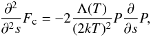 (10)where we have made use of the fact that Λ(T)/(2kT)2 is constant, if a = 2. In hydrostatic equilibrium we can easily estimate how flat the required pressure gradient should be to keep the conductive flux negligible with respect to the other terms in the energy equation; using Eq. (8) in (10), we have
 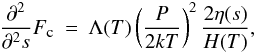 (11)where H(T) is the pressure scale height as function of temperature, defined as H(T) ≡ 2kT/(mHg), and the function η(s) ≡ g ∥ (s)/g(s) is bound in the interval [0, 1]. By imposing the approximate equality between Eh and radiative losses
 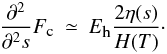 (12)An order of magnitude estimate of the loop dimension is therefore
  (13)where the order of magnitude of the quantities is given by their averages along the loop; factors of the order of unity have been dropped. Thus, the requirement that |∇Fc| ≪ Eh implies that h ≪ H(T), i.e. the height of the loop must be much smaller than the scale height relative to the “average” temperature of the loop. Considering, for example, that the pressure scale height at T = 6 × 10⁴ K is 3.6 Mm and |∇Fc|/Eh is ~0.03 for our loops, then their heights are compatible with this order of magnitude estimation.
In other words, the limitation set to the solutions of Eqs. (8) and (9) by the case Λ(T) ∝ T2, can be circumvented for quasi-static solution, only for low-lying (elongated) loops. Indeed, our solutions with temperatures below 105 K are all a fraction of Mm high (the maximum is ~0.3 Mm, for loops 24–26 in Table 1).
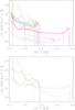 |
Fig. 6 Top: calculated DEMs for the quasi-static cool loops 1–6 (solid black lines), 14–16 (red), 24–26 (green) and the intermediate-temperature loops 17–23 (magenta) of Table 1, compared to the DEMs of the quiet Sun (dashed) and active region (dotted) from the “CHIANTI” atomic data base (Dere et al. 2009). Bottom: total DEMs for each group of loops shown in the top panel. |
3.3. Calculated DEMs for cool and intermediate-temperature loops
The theoretical DEMs for the quasi-static loops we found were computed according to Peter et al. (2006), with a temperature bin of 0.05 dex on a log T scale, and considering a filling factor of 100%:  (14)The upper panel of Fig. 6 shows the calculated DEMs versus temperature of the quasi-static cool loops 1–6 (solid black lines), 14–16 (red), 24–26 (green), and the quasi-static intermediate-temperature loops 17–23 (magenta) of Table 1. In this figure and in the next ones, the calculated DEMs are compared with the observed DEMs of the quiet Sun and active region (dashed and dotted lines, respectively), derived using the Vernazza & Reeves (1978) average quiet Sun and active region intensities, and produced as part of the Arcetri/Cambridge/NRL “CHIANTI” atomic data base collaboration (Dere et al. 2009).
In the lower panel of Fig. 6 we plot the total theoretical DEMs for each group of loops obtained with a different Λ(T) (distinguished by the different colours). Assuming that the loops are equiprobable (uniformly distributed in log T) and with the same cross-section, we divided the temperature range into bins of amplitude 0.2 dex on a log T scale, and considered for each bin a representative loop, i.e. a loop whose maximum temperature belongs to that bin (our loops are almost isothermal). The total DEMs are obtained by summing the DEMs of these representative loops. When more loops have their maximum temperature falling in the same bin, we averaged their DEMs. From Fig. 6, we see that the highest contribution to the total DEM for the cool loops is given essentially by the peaks at maximum temperature and this contribution is determined not by the form of the single loop DEMs, but by the distribution of the emission measures from loop to loop, as predicted by Antiochos & Noci (1986). This is a different behaviour with respect to the hot and the intermediate-temperature loops. The DEM of a group of coronal loops is dominated at all temperatures by the hottest loops, which have the highest emission measure. Hence, the DEM obtained by summing all DEMs will closely resemble the DEM of the hottest loop. For a more accurate discussion on the shape of the resulting DEM from a group of cool and hot loops we refer to the calculations of Antiochos & Noci (1986). They made assumptions on different variables (for example, the magnetic field) and loop distributions that we do not include in our work.
Using ΛAN, we can easily obtain loops with maximum temperatures covering the whole temperature range, from log T ~ 4.1 K up to the position of its peak (log T = 4.95 K). Adding more DEMs of loops with different maximum temperatures, the resulting DEM (black solid line) can be brought to follow the shape of the observed ones. However, using ΛANLyα or ΛDea − H the presence of the Ly-α peak (or a peak in general) at log T ~ 4.2 K produces a relative minimum in all DEMs, which remains in the total DEM (lower panel of Fig. 6, green or red lines). We note that Macpherson & Jordan (1999) derived quiet Sun DEMs that exhibit a shape around log T ~ 4.2 K that resembles the minimum that we find in our results.
The DEMs of the intermediate-temperature loops 20–23 show a minimum at a different temperature with respect to the observed DEMs. We are unable to reproduce the whole observed DEMs considering a unique loop of this kind, in analogy with the relationship between the DEM of a hotter loop and the observed DEM of the corona above 106 K. From Fig. 6 (lower panel), it seems more likely that a combination of the cool and intermediate-temperature loops would assume the right shape to reproduce the observed emission of the lower transition region at the critical turn-up temperature point (T ~ 2 × 10⁵ K) and below T = 105 K. In Fig. 7 we show the total DEM (solid line) resulting from the combination of the DEMs of the cool loops 24–26 plus the intermediate-temperature loops 17–23. We chose to sum the DEMs of these particular cool and intermediate-temperature loops because they were obtained through realistic radiative loss functions. Even though the Λ(T) adopted are different, they can still be combined to obtain a single DEM. We can do this because, while for the existence of the cool loops the shape of Λ(T) under 105 K is very important, we have proved instead that the exact form of the chromospheric radiative losses has little effect on the coronal properties of the loops with temperature higher than 105 K. For loop 17, for example, changing the radiative loss function from ΛDea to ΛDea−H does not change the loop stability and thermodynamic parameters. This result extends what it is already known for hot coronal loops (T > 106 K) and cooling coronal loops (e.g., Reale et al. 1988; Brown 1993).
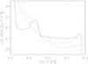 |
Fig. 7 Total DEM resulting from the combination of the DEMs of the loops 17–23 and 24–26 (solid line), compared to the DEMs of the quiet Sun (dashed) and active region (dotted) from the CHIANTI atomic data base (Dere et al. 2009). |
There is a minimum in the total DEM around log T = 4.8 K that is caused by the lack of cool loops with that maximum temperature and ΛDea − H. This minimum almost corresponds to the maximum of the function ΛDea − H or better to the point where its slope starts to change and we have a < 2 (we have already considered the consequences in Sect. 3.2). So, the lack of cool loops with maximum temperature around log T = 4.8 K it is not caused by an incomplete exploration of the parameter space but by the negative slope of ΛDea − H that prevents their formation. We could use the DEMs of the other cool loops of Table 1 with maximum temperature around 6.5 × 10⁴ K or higher but they have been obtained from idealized Λ(T) and would not be suitable for a good comparison with the DEMs of the intermediate-temperature loops 17–23. However, the shape of the averaged DEM of the loops 17–23, with a flat minimum and a tail extended towards low temperatures, helps filling this gap, improving the agreement with the observed DEM. Since we considered a filling factor of 100% the total DEM has its highest value. With a lower filling factor the height of the DEM would be lower.
4. Conclusions
We have studied the conditions of existence and stability of cool loops with T ≲ 105 K through hydrodynamic simulations, finding that it is possible to obtain quasi-static (velocities lower than 1 km s-1) cool loops, as predicted by Antiochos & Noci (1986), stable over hours or more. These loops have been obtained by using different dependences of the radiative loss function on the temperature with respect to the work of Cally & Robb (1991). We obtained stable quasi-static loops even in conditions judged prohibitive by the same authors on the basis of an analysis of strictly static and stationary loop equations. We examined and discussed the quasi-static solutions we found, and showed that their existence is caused indeed by the small departures from static conditions, i.e. to the presence of a small but non-zero conductive flux and velocities, and to quite stringent constraints on the pressure gradients. In fact, for low-temperature loops, the requirement of nearly constant pressure implies that these loops can exist only if they are limited to low heights above the chromosphere (a fraction of Mm). We also show that the presence of the peak caused by the Ly-α losses in the radiative loss function does not preclude the existence of cool loops. Moreover, we analyzed the contributions of cool loops to the TR DEM, showing that the emission of these kind of loops can account for the observed DEM at T < 105 K, if they were uniformly distributed.
The cool loops found cannot be related to any of the observations present in the literature because of their dimensions and especially because of their low heights. We find cool loops with lengths of 5–10 Mm, but with very low heights (in the range 10-2−10-1 Mm). Loops this low in the solar atmosphere (effectively embedded in the chromosphere) cannot be visible in the Ly-α line; moreover, compared with the observations of Patsourakos et al. (2007), our loops typically have lower pressures compared to their estimates.
Indeed, the shape of the cool loops we found could give information on the orientation of the magnetic field in the transition region, and in particular on its inclination. Since, as already pointed out, these loops are very flat, the magnetic flux tube should emerge at transition region temperatures with a quite small angle with respect to the Sun’s surface and observations should reveal a predominance of horizontal magnetic field direction at their height levels, assuming that these loops are almost everywhere.
We also obtained quasi-static loops with maximum temperature in the range 2 × 10⁵−106 K, using a realistic radiative loss function. These loops are smaller with respect to coronal loops but have different characteristics compared to the static cool loops proposed by Antiochos & Noci (1986) and others. These loops in principle could be observed with current telescopes, but in order to resolve them in all their temperature extension, we would need multi-temperature observations, i.e. different UV lines formed at temperatures between 105−106 K with resolution of at least 1′′. Loops 17 and 18 have their maximum temperature around 2.5 × 10⁵ K, which is the upper limit of the region in which Feldman (1983) located the “UFS (unresolved fine structures)”. We find that these intermediate-temperature loops follow the scaling laws for coronal loops contrary to results of previous works based on the observational data (e.g., Brown 1996). The loops obtained have indeed low pressures that make their parameters obey the RTV scaling laws, but these pressures are 1–2 orders of magnitudes lower than those estimated from observations (Brown 1996). Observed intermediate-temperature loops are usually associated with flows while we were studying possible solutions to the hydrodynamic equations in quasi-static conditions without considering their role. The low values of the pressure we found for these loops are the only possible option to find solutions to the hydrodynamic equations in quasi-static conditions. Owing to their low pressures, these loops obey to the scaling laws for coronal loops. The presence of substantial flows could influence their pressures.
We are not able to reproduce the DEMs derived from observations with only one set of parameters (a single loop). A similar problem has already been reported in the paper of Susino et al. (2010) but for coronal loops. We find instead that a combination of cool and intermediate-temperature loops, precisely because of their computed pressures, can give a DEM with a shape not too far from the observed one. Of course this does not preclude the possibility that some additional physical processes, not included in our simulations (such as those proposed by Judge 2008; or by Klimchuk et al. 2008; and De Pontieu et al. 2009, or dynamic structures such as cooling, heating loops and spicules), must be taking place in the transition region and contribute to explain the discrepancies with the observed DEM structure. Owing to their dimensions, the emission of the quasi-static loops found can be seen as a diffuse component of the transition region.
In our simulations, we considered only the case of constant heating rate and we have already found quasi-static cool loops in conditions not allowed from strictly static and stationary hydro-dynamical equations. More realistic assumptions could facilitate obtaining stable, quasi-static cool loops. In particular, we showed that the shape of the radiative loss function below 105 K is very important for the existence of cool loops. Because the radiative losses around log T ~ 4.2 K are dominated by the H i Ly-α, we plan to explore the effect on the structure and stability of cool loops in a follow-up study with a more realistic treatment of hydrogen radiation losses in the lower TR. To do so, it will be necessary to improve the models by introducing a full treatment of optically thick radiative losses and/or partial ionization, and therefore solving the radiative transfer equations and rate equations of hydrogen (non-local thermodynamic equilibrium). Our first attempt to simulate an optically thick radiative loss function by removing the hydrogen losses from a realistic radiative loss function seems to be promising. Without the hydrogen losses, the function ΛDea−H becomes lower and we are able to obtain quasi-static cool loops with T < 105 K.
Taking into account finite cross sections for these loops could influence the details of the radiative transfer in the Ly-α line (by reducing, for instance, the escape probability of Ly-α photons). Predicting the effect of loop area expansion above the chromosphere is challenging, although it is difficult to envision substantial expansion factors in such small loops.
Finally, the maximum temperature reachable by cool loops is limited only by the second maximum (or a change of slope) present in the Λ(T) because we have shown that the peak caused by the Ly-α losses is not a limit. The different radiative loss functions used have this maximum (or the slope change) at different temperatures. So, we underline the importance of knowing accurately the Λ(T) also at temperature around 105 K for the structure of the cool loops and of what we termed “intermediate loops”, in analogy with the importance of the position and strength of the Ly-α peak for cool loops.
Acknowledgments
This work was supported by the ASI/INAF contracts I/05/07/0 for the program “Studi Esplorazione Sistema Solare”, and I/023/09/0 for the program “Attività scientifica per l’analisi dati Sole e plasma – Fase E2/F”.
References
- Akiyama, S., Doschek, G. A., & Mariska, J. T. 2005, ApJ, 623, 540 [NASA ADS] [CrossRef] [Google Scholar]
- Antiochos, S. K., & Noci, G. 1986, ApJ, 301, 440 [NASA ADS] [CrossRef] [Google Scholar]
- Antiochos, S. K., MacNeice, P. J., Spicer, D. S., & Klimchuk, J. A. 1999, ApJ, 512, 985 [NASA ADS] [CrossRef] [Google Scholar]
- Athay, R. G. 1981, ApJ, 249, 340 [NASA ADS] [CrossRef] [Google Scholar]
- Brekke, P., Kjeldseth-Moe, O., & Harrison, R.A. 1997, Sol. Phys., 175, 511 [NASA ADS] [CrossRef] [Google Scholar]
- Brown, S. F. 1993, Ph.D. Thesis, The University of Sydney [Google Scholar]
- Brown, S. F. 1996, A&A, 305, 649 [NASA ADS] [Google Scholar]
- Bryans, P., Landi, E., & Savin, D. W. 2009, ApJ, 691, 1540 [NASA ADS] [CrossRef] [Google Scholar]
- Cally, P. S., & Robb, T. D. 1991, ApJ, 372, 329 [NASA ADS] [CrossRef] [Google Scholar]
- Carlsson, M., & Stein, R. F. 1992, ApJ, 397, L59 [NASA ADS] [CrossRef] [Google Scholar]
- Colgan, J., Abdallah, J., Jr., Sherrill, M. E., et al. 2008, ApJ, 689, 585 [NASA ADS] [CrossRef] [Google Scholar]
- Cook, J. W., Cheng, C.-C., Jacobs, V. L., & Antiochos, S. K. 1989, ApJ, 338, 1176 [NASA ADS] [CrossRef] [Google Scholar]
- De Pontieu, B., Hansteen, V. H., McIntosh, S. W., & Patsourakos, S. 2009, ApJ, 702, 1016 [NASA ADS] [CrossRef] [Google Scholar]
- Dere, K. P. 1982, Sol. Phys., 75, 189 [NASA ADS] [CrossRef] [Google Scholar]
- Dere, K. P., Landi, E., Young, P. R., et al. 2009, A&A, 498, 915 [NASA ADS] [CrossRef] [EDP Sciences] [Google Scholar]
- Di Giorgio, S., Reale, F., & Peres, G. 2003, A&A, 406, 323 [NASA ADS] [CrossRef] [EDP Sciences] [Google Scholar]
- Dowdy, J. F., Jr. 1993, ApJ, 411, 406 [NASA ADS] [CrossRef] [Google Scholar]
- Dowdy, J. F., Jr., Rabin, D., & Moore, R. L. 1986, Sol. Phys., 105, 35 [NASA ADS] [CrossRef] [Google Scholar]
- Durrant, C. J., & Brown, S. F. 1989, PASA, 8, 137 [NASA ADS] [Google Scholar]
- Feldman, U. 1983, ApJ, 275, 367 [NASA ADS] [CrossRef] [Google Scholar]
- Feldman, U., Dammasch, I. E., & Wilhelm, K. 2001, ApJ, 558, 423 [NASA ADS] [CrossRef] [Google Scholar]
- Fontenla, J. M., Avrett, E. H., & Loeser, R. 1993, ApJ, 406, 319 [NASA ADS] [CrossRef] [Google Scholar]
- Foukal, P.V. 1976, A&A, 210, 575 [Google Scholar]
- Gabriel, A. H. 1976, Philos. Trans. R. Soc. London A, 281, 339 [Google Scholar]
- Gaetz, T. J., & Salpeter, E. E. 1983, ApJS, 52, 155 [NASA ADS] [CrossRef] [Google Scholar]
- Hood, A. W., & Priest, E. R. 1979, A&A, 77, 233 [NASA ADS] [Google Scholar]
- Judge, P. 2008, ApJ, 683, L87 [NASA ADS] [CrossRef] [Google Scholar]
- Judge, P., & Centeno, R. 2008, ApJ, 687,1388 [NASA ADS] [CrossRef] [Google Scholar]
- Klimchuk, J. A., Antiochos, S. K., & Mariska, J. T. 1987, ApJ, 320, 409 [NASA ADS] [CrossRef] [Google Scholar]
- Klimchuk, J. A., Patsourakos, S., & Cargill, P. J. 2008, ApJ, 682, 1351 [Google Scholar]
- Korendyke, C. M., Vourlidas, A., Cook, J. W., et al. 2001, Sol. Phys., 200, 63 [NASA ADS] [CrossRef] [Google Scholar]
- Litwin, C., & Rosner, R. 1993, ApJ, 412, 375 [Google Scholar]
- Lanzafame, A. C., Brooks, D. H., Lang, J., et al. 2002, A&A, 384, 242 [NASA ADS] [CrossRef] [EDP Sciences] [Google Scholar]
- Lanzafame, A. C., Brooks, D. H., & Lang, J. 2005, A&A, 432, 1063 [NASA ADS] [CrossRef] [EDP Sciences] [Google Scholar]
- McClymont, A. N., & Canfield, R. C. 1983, ApJ, 265, 497 [NASA ADS] [CrossRef] [Google Scholar]
- MacNeice, P. J., Olson, K. M., Mobarry, C., de Fainchtein, R., & Packer, C. 2000, Comput. Phys. Commun., 126, 330 [NASA ADS] [CrossRef] [Google Scholar]
- Macpherson, K. P., & Jordan, C. 1999, MNRAS, 308, 510 [NASA ADS] [CrossRef] [Google Scholar]
- Patsourakos, S., Gouttebroze, P., & Vourlidas, A. 2007, ApJ, 664, 121 [Google Scholar]
- Peter, H., Gudiksen, B. V., & Nordlund, A. 2004, ApJ, 617, 85 [Google Scholar]
- Peter, H., Gudiksen, B. V., & Nordlund, A. 2006, ApJ, 638, 1086 [NASA ADS] [CrossRef] [MathSciNet] [Google Scholar]
- Reale, F. 2010, Liv. Rev. Sol. Phys., 7, 5 [Google Scholar]
- Reale, F., Peres, G., Serio, S., Rosner, R., & Schmitt, J. H. M. M. 1988, ApJ, 328, 256 [NASA ADS] [CrossRef] [Google Scholar]
- Rosner, R., Tucker, W. H., & Vaiana, G. S. 1978, ApJ, 220, 643 [NASA ADS] [CrossRef] [Google Scholar]
- Serio, S., Peres, G., Vaiana, G. S., Golub, L., & Rosner, R. 1981, ApJ, 243, 288 [NASA ADS] [CrossRef] [Google Scholar]
- Spadaro, D., Lanza, A. F., Lanzafame, A. C., et al. 2003, ApJ, 582, 486 [NASA ADS] [CrossRef] [Google Scholar]
- Spadaro, D., Lanza, A. F., Karpen, J. T., & Antiochos, S. K. 2006, ApJ, 642, 579 [NASA ADS] [CrossRef] [Google Scholar]
- Susino, R., Lanzafame, A. C., Lanza, A. F., & Spadaro, D. 2010, ApJ, 709, 499 [NASA ADS] [CrossRef] [Google Scholar]
- Vernazza, J. E., & Reeves, E. M. 1978, ApJS, 37, 485 [NASA ADS] [CrossRef] [Google Scholar]
- Vernazza, J. E., Avrett, E. H., & Loeser, R. 1981, ApJS, 45, 635 [NASA ADS] [CrossRef] [Google Scholar]
- Vourlidas, A., Sanchez Andrade-Nuño, B., Landi, E., et al. 2010, Sol. Phys., 261, 53 [NASA ADS] [CrossRef] [Google Scholar]
All Tables
All Figures
|
Fig. 1 Radiative loss functions considered in this work. Solid line: power-law segments function, equal to T2 (for log T < 4.95 K) and T-1 (for log T > 4.95 K); solid line plus star symbols: a peak mimicking the H Ly-α losses was added to the previous function; dashed line: from Cook et al. (1989), but with a T3 dependence below T = 105 K; long-dashed line: from Colgan et al. (2008); dotted line: from Dere et al. (2009); dot-dashed line: from Dere et al. (2009) without the H contribution. |
| In the text | |
|
Fig. 2 Top panel, left: temperature (solid line) and pressure (dashed line) as a function of the curvilinear coordinate along the field lines, s. Right: divergence of the conductive flux (asterisks), radiative losses (crosses) and constant heating rate, Eh (solid line), as a function of the temperature, for loop 4. Middle and bottom panels: as in the top panels for loop 10 and 15, respectively. |
| In the text | |
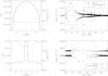 |
Fig. 3 As in Fig. 2 for loop 17 (top panels) and loop 25 (bottom panels). |
| In the text | |
|
Fig. 4 Behaviour of the physical parameters for loops 1–6 (diamonds), 7–13 (crosses), 14–16 (triangles), 17–23 (asterisks) and 24–26 (squares) of Table 1. The solid lines represent the RTV scaling laws for coronal loops for different values of L/2. The dotted line represents Eh = P2. |
| In the text | |
|
Fig. 5 Evolution of the maximum temperature of loop 11 in Table 1 during the hydrodynamic simulation. The horizontal solid line indicates the break temperature log T = 4.95 K. |
| In the text | |
|
Fig. 6 Top: calculated DEMs for the quasi-static cool loops 1–6 (solid black lines), 14–16 (red), 24–26 (green) and the intermediate-temperature loops 17–23 (magenta) of Table 1, compared to the DEMs of the quiet Sun (dashed) and active region (dotted) from the “CHIANTI” atomic data base (Dere et al. 2009). Bottom: total DEMs for each group of loops shown in the top panel. |
| In the text | |
|
Fig. 7 Total DEM resulting from the combination of the DEMs of the loops 17–23 and 24–26 (solid line), compared to the DEMs of the quiet Sun (dashed) and active region (dotted) from the CHIANTI atomic data base (Dere et al. 2009). |
| In the text | |
Current usage metrics show cumulative count of Article Views (full-text article views including HTML views, PDF and ePub downloads, according to the available data) and Abstracts Views on Vision4Press platform.
Data correspond to usage on the plateform after 2015. The current usage metrics is available 48-96 hours after online publication and is updated daily on week days.
Initial download of the metrics may take a while.