| Issue |
A&A
Volume 537, January 2012
|
|
|---|---|---|
| Article Number | A48 | |
| Number of page(s) | 10 | |
| Section | Extragalactic astronomy | |
| DOI | https://doi.org/10.1051/0004-6361/201117168 | |
| Published online | 09 January 2012 | |
The scaling relation between the mass of supermassive black holes and the kinetic energy of random motions of the host galaxies
1 Max-Planck-Institute for Astronomy, Königstuhl 17, 69117 Heidelberg, Germany
e-mail: This email address is being protected from spambots. You need JavaScript enabled to view it.
2 Department of Physics, University of Salerno, via Ponte Don Melillo, 84084 Fisciano (SA), Italy
3 Department of Engineering, University of Sannio, Piazza Roma 21, 82100 Benevento, Italy
e-mail: This email address is being protected from spambots. You need JavaScript enabled to view it.
Received: 2 May 2011
Accepted: 13 October 2011
Abstract
Context. Thanks to the improved angular resolution of modern telescopes and kinematic models, the existence of supermassive black holes (SMBHs) in the inner part of galaxies, regardless their morphology and nuclear activity, has been established on quite solid grounds. A possible correlation between the mass of SMBHs (M•) and the evolutionary state of their host galaxies is expected and is currently under a heated debate.
Aims. Based on the recent 2D decomposition of 3.6 μm Spitzer/IRAC images of local late- and early-type galaxies with M• measurements, we investigated various scaling laws, studying what is the best predictor of the mass of the central black holes, that is the one with the lowest value of intrinsic scatter. In particular, we focused on the M• − MGσ2 law, that is the relation between the mass of SMBHs and the kinetic energy of random motions of the corresponding host galaxies, MG is the mass and σ the velocity dispersion of the host galaxy (bulge).
Methods. In order to find the best fit for each of the scaling laws examined, we performed a least-squares regression of M• on x for the considered sample of galaxies, x being a whatever known parameter of the galaxy bulge. For this purpose, we made use of both the linear regression LINMIX_ERR and FITEXY methods.
Results. Our analysis shows that M• − MGσ2 law fits the examined experimental data successfully as much as the other known scaling laws (all correlations have similar intrinsic scatters within the errors) and shows a value of χ2 (estimated by FITEXY) better than the others, a result which is consistent with previous determinations at shorter wavelengths. This means that a combination of σ and MG (or Re) could be necessary to drive the correlations between M• and other bulge properties. This issue has been investigated by a careful, although not fully conclusive, analysis of the residuals of the various relations.
Conclusions. In order to avoid rushed conclusions on galaxy activity and evolution, the indirect inferring of the masses of the supermassive black holes from the kinetic energy of random motions via the M• − MGσ2 relation should be considered, especially when applied to higher redshift galaxies (z > 0.01). This statement is suggested by a reanalysis of Sloan Digital Sky Survey (SDSS) data used to study the black hole growth in the nearby Universe. By adopting the M• − MGσ2 relation instead of the M• − σ relation, a radio-quiet/radio-loud dichotomy appears in the SMBH mass distribution of the corresponding SDSS early-type AGN galaxies.
Key words: black hole physics / galaxies: active / galaxies: kinematics and dynamics / galaxies: statistics / galaxies: evolution / galaxies: general
© ESO, 2012
1. Introduction
Scaling laws in galaxies are important to describe the mechanisms for the initial formation of the first galaxies as well as for their cosmic evolution. They also apply quite well to high redshifts, implying that the interaction and merging processes must, at least on average, preserve them (Schneider 2006).
One of the recent successes in extragalactic astronomy was the discovery that both early- and late-type galaxies, close (<100 Mpc) to the Milky Way, host a supermassive black hole (SMBH; M• > 106 M⊙) at their center (Kormendy & Richstone 1995; Richstone et al. 1998). Subsequently, based on more and more precise experimental data, it was possible to draw up many galaxy data sets, containing measures of the SMBH masses as well as the structural parameters of the host galaxies (bulges) (Magorrian et al. 1998; Tremaine et al. 2002; Marconi & Hunt 2003; Gebhardt et al. 2003; Häring & Rix 2004; Aller & Richstone 2007; Graham 2008a,b; Hu 2008; Kisaka et al. 2008; Feoli & Mancini 2009; Gültekin et al. 2009a; Beifiori et al. 2009, 2011).
Thanks to these catalogues, the astrophysical community identified a large number of scaling laws, in which the mass of SMBHs correlates with several properties of the host spheroidal component1, such as for instance bulge luminosity, mass, effective radius, central potential, dynamical mass, concentration, Sersic index, binding energy, etc. (Richstone et al. 1998; Magorrian et al. 1998; Ferrarese & Merritt 2000; Gebhardt et al. 2000; Laor 2001; Merritt & Ferrarese 2001; Wandel 2002; Tremaine et al. 2002; Marconi & Hunt 2003; Häring & Rix 2004; Graham & Driver 2005; Feoli & Mele 2005; Aller & Richstone 2007; Hopkins et al. 2007b). Another scaling law has been recently proposed, the M• − Reσ3 law (Feoli & Mancini 2011), which is based on a pure theoretical framework, and is on the wake of the numerical results of Hopkins et al. (2007a).
Relations between M• and X-ray luminosity, radioluminosity (Gültekin et al. 2009b), momentum parameter (Soker & Meiron 2011), number of globular clusters (Burkert & Tremaine 2010; Snyder et al. 2011) have also been presented, whereas the correlation with the dark matter halo is still a matter of controversy (Ferrarese 2002; Baes et al. 2003; Kormendy & Bender 2011; Graham 2011; Volonteri et al. 2011; Bellovary et al. 2011).
All these scaling laws have led to the belief that SMBH growth and bulge formation regulate each other (Ho 2004), even if it is difficult to understand the fundamental nature of the correlations between SMBHs and host properties (Jahnke & Macciò 2011), also because all such relations depend critically on the accuracy of the published error estimates in all quantities under consideration (Novak et al. 2006; Lauer et al. 2007).
Just as the Faber-Jackson relation, the “traditional” relation between the SMBH mass and bulge velocity dispersion σ or stellar mass M ⋆ should be projections of the same fundamental plane relation. Current observations require a correlation of the form  over a simple correlation with either σ or M ⋆ at ≥ 3σ confidence (Hopkins et al. 2007a; Hopkins 2008; Marulli et al. 2008).
Actually, another competitive correlation, as opposed to the popular M• − M ⋆ and M• − σ, between M• and the kinetic energy of random motions of the corresponding bulges, i.e. M ⋆ σ2, has been advanced (Feoli & Mele 2005; Feoli & Mancini 2009). This relation has also a plausible physical interpretation that resembles the H-R diagram: the mass of the central SMBH, just like entropy, can only increase with time or at most remain the same but never decrease; M• is therefore related to the age of the galaxy. On the other hand, the kinetic energy of the stellar bulges directly determines the temperature of the galactic system. The goodness of the M• − M ⋆ σ2 relation, as a predictor of the SMBH mass in the center of galaxies, has been already tested, with clear positive results, over three independent galaxy samples and in the framework of the ΛCDM cosmology, using two galaxy formation models based on the Millennium Simulation, one by Bower et al. (2006) (the Durham model) and the other by De Lucia & Blaizot (2007) (the MPA model) (Feoli et al. 2011).
Recently, Sani et al. (2011) have presented a mid-infrared investigation of the scaling relations between SMBH masses and some of structural parameters (luminosity, mass, effective radius, velocity dispersion) of the host spheroids in local galaxies, based on Spitzer/IRAC 3.6 μm images of 57 galaxies of different morphological types with M• measurements. Their results were consistent with the above mentioned determinations at shorter wavelengths.
The present work has several aims. First of all, we used the data set of Sani et al. (2011) and completed their study, by analyzing the other known scaling relations that involve bulge properties: kinetic energy M• − M ⋆ σ2, momentum parameter M• − M ⋆ σ (Soker & Meiron 2011), and the M• − Reσ3 law. In order to have a comprehensive study, we also reanalyzed the relations already investigated by Sani et al. (2011). This allows us to have a rapid comparison among the various relationships and to find what is the tightest.
Secondly, we examined if a simple one-to-one correlation between, e.g., M• and σ is an exhaustive description of the Sani et al. (2011) data, or if we have to consider an additional dependence on a second parameter such as Re or M ⋆ . In order to study the existence of such a dependence, we used both the approach of Marconi & Hunt (2003), who investigated the correlation of the residual of the M• − σ relation with Re and M ⋆ , and that of Hopkins et al. (2007a), who considered the correlations between residuals at fixed σ.
Finally, by considering the same Sloan Digital Sky Survey (SDSS) data set, used by Schawinski et al. (2010) to study the role of SMBH growth in the evolution of normal and active galaxies, we discuss the possible consequences of the use of the scaling law M• − M ⋆ σ2 in the place of M• − σ in inferring the SMBH masses.
The paper is structured as follows. In Sect. 2 we describe the galaxy sample examined and the fitting procedures performed to find the best-fitting lines for each of the relationships considered. In Sect. 3 we report the fitting parameters and show the plots of the various scaling relations. The issue related the existence of a SMBH fundamental plane is tackled in Sect. 4. In order to emphasize how the conclusions could be different using a scaling law rather than another one, in Sect. 5 we remake the analysis performed by Schawinski et al. (2010) on SDSS data. After that, we draw our conclusions in Sect. 6.
2. Data analysis
An important fact that emerges from the Spitzer/IRAC images, analyzed by Sani et al. (2011), is that the 3.6 μm luminosity proved to be a very good tracer of stellar mass. Actually, this is a crucial information in order to perform a proper 2D photometric decomposition of the galaxy components (disk, bar, bulge, etc.), which is useful to investigate the interplay between central SMBHs and the evolutionary state, luminosity and dynamics of their host galaxies.
Thanks to this bulge-disk decomposition, the authors were also able to identify in their sample 9 disk galaxies that host a pseudobulge2, i.e. Circinus, IC 2560, NGC 1068, NGC 3079, NGC 3368, NGC 3489, NGC 3998, NGC 4258, and NGC 4594. Constructing the correlation between M• and the bulge 3.6 μm luminosity L3.6,bul, Sani et al. (2011) noticed that four of these nine are consistent with classical-bulge galaxies, whereas the other 5 are outliers at more than 4σ below their linear regression. These galaxies are Circinus, IC 2560, NGC 1068, NGC 3079, and NGC 3368. This result is consistent with the fact that the M• − σ relation for pseudobulges is different from the relation in the classical bulges at a significance level > 3σ (Hu 2008), and that at a fixed bulge mass, M• in pseudobulges are on average more than one magnitude smaller than the ones in classical bulges (Hu 2009). Moreover the elliptical-only galaxies, and the non-barred galaxies, define tighter relations with less scatter and a reduced slope than the one obtained when using a full galaxy sample (Graham 2008b; Graham et al. 2011). For these reasons, we neglected from the sample of Sani et al. (2011) the above mentioned 5 galaxies and thus considered a more consistent sample of N = 52 galaxies, which is therefore formed by 24 ellipticals, 3 dwarf ellipticals (dEs), 11 lenticulars, 6 barred lenticulars, 4 spirals, and 4 barred spirals. On the contrary the fits in the paper of Sani et al. (2011) considered only 48 objects excluding all the nine pseudobulges.
By using this sample (all the parameters are reported in Tables 2 and 3 of Sani et al. 2011), we investigated what the relationship that best predicts the black hole mass is. In particular, the relations that we want to study can be written in the following form  (1)where m is the slope, b is the normalization, and x is a parameter of the host bulge. Equation (1) can be used to predict the values of M• in other galaxies once we know the value of x. In order to minimize the scatter in the quantity to be predicted, we have to perform an ordinary least-squares regression of M• on x for the considered galaxies, of which we already know both the quantities. We considered error bars in both variables and, to simplify the analysis, we make all of them symmetric about the preferred value by averaging the size of the upper and lower 1σ error bars so that
  becomes x ± (h + l)/2. To obtain the parameters of the fits (m and b), we adopted the following three different fitting methods.
-
1)
The linear regression routine FITEXY (Presset al. 1992) for the relationy = b + mx, by minimizing the χ2
 (2)The most efficient and unbiased estimate of the slope is obtained when the fitting method incorporates the residual variance, also known as intrinsic scatter ε0, which is that part of the variance which cannot be attributed to specific causes (Novak et al. 2006). So, if the reduced
  of the fit is not equal to 1, we normalize including the suitable value of ε0 in the Eq. (2) to obtain
  (3)Lastly, it is possible to obtain an estimate of the 1σ error bar on ε0 by adjusting it until the
  is equal to 1 + (2/N)1/2.
 -
2)
The linear regression FITEXY method as modified by Tremaine et al. (2002), where the measurement errors of the dependent variable and the intrinsic scatter are added in quadrature, adjusting ε0 and refitting until the reduced χ2 of the fit is equal to 1.
-
3)
The Bayesian linear regression routine LINMIX_ERR (Kelly 2007) to determine the slope, the normalization, and the intrinsic scatter of the relationship
 (4)This routine approximates the distribution of the independent variable as a mixture of Gaussians, bypassing the assumption of a uniform prior distribution on the independent variable, which is used in the derivation of χ2-FITEXY minimization routine. Since a direct computation of the posterior distribution is too computationally intensive, random draws from the posterior distribution are obtained using a Markov Chain Monte Carlo method (Kelly 2007).
In order to be consistent with the results reported by Sani et al. (2011), we used the LINMIX_ERR as the favorite routine to calculate the fitting parameters of the SMBH-bulge scaling relations.
In Eq. (1) in place of x we considered the following quantities: σ, Mdyn, M ⋆ , Mdynσ, M ⋆ σ, Mdynσ2, M ⋆ σ2, Reσ3. Mdyn is the bulge dynamical mass, which Sani et al. (2011) assumed dominated by stellar matter with a negligible contribution of dark matter and gas, and computed as:  (5)where G is the gravitational constant, while the factor k was fixed by the authors to be equal to 5, in agreement with Cappellari et al. (2006). On the contrary, the stellar mass M ⋆ of each galaxy has been estimated by combining the bulge 3.6 μm luminosity with the galaxy mass-to-light ratio (M/L); the values are reported in Table 1 (Sani & Marconi, priv. comm.). We follow Sani et al. (2011) in this choice, even if we would have preferred an estimate of masses by means of the Jeans equation or Schwarzschild methods as in (Feoli & Mancini 2009), because the use of Eq. (5) makes the relations M• − Mdynσ and M• − Reσ3, which are deduced from different theoretical contexts, practically equivalent.
3. Results
Referring to the sample of 52 galaxies, in Table 2 we collected the parameters of the fits obtained thanks to the three above mentioned fitting methods for the various relations that we analyzed, together with the corresponding values of the χ2, the intrinsic scatter ε0, and the Pearson linear correlation coefficient r. In Figs. 1 − 4, we reported the relations in log-log plots (we associated a particular marker to each galaxy according to its morphological type). The best-fitting lines are also shown for each diagram.
The relations between M• and the corresponding kinetic energy, momentum parameter, velocity dispersion, galaxy mass and Reσ3, fitted with a Bayesian approach to linear regression are: ![Mathematical equation: \begin{eqnarray*} && \log_{10}\!M_{\bullet} \!=\! (5.30\, \!\pm\! \,0.26) \!+ \! (0.63\, \!\pm\!\, 0.05) \!\times\! \log_{10}\left[M_{{\rm dyn}}\sigma^2/M_{\odot}\,c^2\right]; \\ && \hspace*{6cm} (\varepsilon_{0}=0.30 \pm 0.16) \\ && \log_{10}M_{\bullet} \!=\! (5.18 \pm 0.27)+(0.65 \pm 0.06) \!\times\! \log_{10}\left[M_{\star}\,\sigma^2/M_{\odot}\,c^2\right]; \\ && \hspace*{6cm} (\varepsilon_{0}=0.30 \pm 0.16) \\ && \log_{10}M_{\bullet} \!=\! (8.29 \pm 0.05)+(3.95 \pm 0.31) \!\times\! \log_{10}\left[\sigma/200~{\rm km\,s^{-1}}\right]; \\ && \hspace*{6cm} (\varepsilon_{0} = 0.31 \pm 0.16), \\ && \log_{10}M_{\bullet} \!=\! (3.15 \pm 0.47)+(0.71 \pm 0.07) \!\times\! \log_{10}\left[R_{{\rm e}}\,\sigma^{3}/c\,G\,M_{\odot}\right]; \\ && \hspace*{6cm} (\varepsilon_{0} = 0.33 \pm 0.17), \\ && \log_{10}M_{\bullet} \!=\! (2.64 \pm 0.53)+(0.71 \pm 0.07) \!\times\! \log_{10}\left[M_{{\rm dyn}}\,\sigma/M_{\odot}\,c\right]; \\ && \hspace*{6cm} (\varepsilon_{0} = 0.33 \pm 0.17), \\ && \log_{10}M_{\bullet} \!=\! (2.47 \pm 0.54)+(0.73 \pm 0.07) \!\times\! \log_{10}\left[M_{\star}\,\sigma/M_{\odot}\,c\right]; \\ && \hspace*{6cm} (\varepsilon_{0} = 0.34 \pm 0.17), \\ && \log_{10}\!M_{\bullet} \!=\! (8.18\, \!\pm\! \,0.06)\!+\!(0.80\, \!\pm\!\, 0.09) \!\times\! \left(\log_{10}\!\left[M_{{\rm dyn}}/M_{\odot}\right]\!-\!11\!\right); \\ && \hspace*{6cm} (\varepsilon_{0} = 0.38 \pm 0.19), \\ && \log_{10}\!M_{\bullet} \!=\! (8.15 \pm 0.06)\!+\!(0.80 \pm 0.09) \!\times\! \left(\log_{10}\left[M_{\star}/M_{\odot}\right]\!-\!11\right); \\ && \hspace*{6cm} (\varepsilon_{0}=0.40 \pm 0.19). \end{eqnarray*}](/articles/aa/full_html/2012/01/aa17168-11/aa17168-11-eq59.png) \arraycolsep1.75ptBy inspection of Table 2, it is possible to note that all the fitting parameters are consistent with previous determinations from the literature at shorter wavelengths. The 3.6 μm M• − Mdynσ2 relation looks to be slightly preferable compared with the other M• − bulge relations, especially if one considers the values of
\arraycolsep1.75ptBy inspection of Table 2, it is possible to note that all the fitting parameters are consistent with previous determinations from the literature at shorter wavelengths. The 3.6 μm M• − Mdynσ2 relation looks to be slightly preferable compared with the other M• − bulge relations, especially if one considers the values of  estimated by FITEXY (Col. 5). However, since all correlations have similar intrinsic scatters within the errors (Col. 6), we cannot conclusively determine what the best one is.
4. A possible fundamental plane for supermasssive black holes
By analyzing a sample of 27 galaxies, which are deemed to have “secure” SMBH and bulge mass measurements, Marconi & Hunt (2003) were the first to note that M• is significantly correlated both with σ and with Re. Plotting the residuals of the M• − σ correlation against Re, they concluded that a combination of σ and Re was necessary to drive the correlations between M• and other bulge properties. This topic was then theoretically investigated by Hopkins et al. (2007a) by simulations of major galaxy mergers, which defined a fundamental plane (FP), analogous to the FP of elliptical galaxies, of the form  or
or  , and by Marulli et al. (2008) who found M• ∝ (M ⋆ σ2)0.7. 3 Moreover, the sample of Marconi & Hunt (2003) was reanalyzed by Hopkins et al. (2007b), who found that the observations define a FP that should be preferred over a simple relation between SMBH and any of σ, Mdyn, M ⋆ , or Re alone at > 3σ (99.9%) significance.
The values of the stellar mass and 1σ error for each galaxy of the sample (Sani & Marconi 2011, priv. comm.).
Regression results for log M• = b + mlog x with a sample composed by 52 galaxies.
 |
Fig. 1 M• − Mdynσ2 (left) and M• − M ⋆ σ2 (right) relations for the sample of N = 52 galaxies extracted from the data set of Sani et al. (2011). The symbols represent elliptical galaxies (red ellipses), lenticular galaxies (green circles), barred lenticular galaxies (dark green circles), spiral galaxies (blue spirals), barred spiral galaxies (dark blue barred spirals), and dwarf elliptical galaxies (orange ellipses). The black lines are the lines of best fit. |
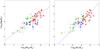 |
Fig. 2 M• − Mdyn (left) and M• − M ⋆ (right) relations for the sample of N = 52 galaxies extracted from the data set of Sani et al. (2011). The symbols are the same as in Fig. 1. |
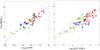 |
Fig. 3 M• − σ200 (left) and M• − Reσ3 (right) relations for the sample of N = 52 galaxies extracted from the data set of Sani et al. (2011). The symbols are the same as in Fig. 1. |
However, Aller & Richstone (2007) noticed that the M• − M•(σ) residuals for their sample of 23 galaxies did not indicate the combination suggested by Marconi & Hunt (2003). The evidence of a correlation between the residuals and the effective radius is obtained by considering only spiral and lenticular bulges. Graham (2008b) reached the same result studying a sample of 40 galaxies. In particular he found that the barred galaxies are responsible for much of the trend between the M• − σ residuals and Re, whereas the elliptical galaxies alone do not provide substantial support for the existence of a FP plane for SMBHs. The analysis of Sani et al. (2011) does not confirm the existence of a FP. In fact, comparing the residuals of M• − σ for bulges with their effective radius, they did not found any significant correlation either for the entire sample (r = 0.29), or excluding barred galaxies and/or pseudobulges (r = 0.20 − 0.29).
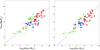 |
Fig. 4 M• − Mdynσ (left) and M• − M ⋆ σ (right) relations for the sample of N = 52 galaxies extracted from the data set of Sani et al. (2011). The symbols are the same as in Fig. 1. |
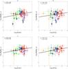 |
Fig. 5 Residuals of M• − σ as a function of the host galaxy effective radius Re (left) and stellar mass M ⋆ (right), for the full sample of 57 galaxies (a − b), and for a more consistent sample (see text) of 52 galaxies (c–d), respectively. The corresponding intrinsic scatter and Pearson linear coefficient are reported in the upper-left corner of each plot. The symbols are the same as in Fig. 1. Galaxies inside the black circles are pseudo-bulges. |
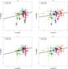 |
Fig. 6 Correlations between the residuals in the M• − σ and Re − σ (left), and M ⋆ − σ (right) relations at each σ (Hopkins et al. 2007b), for the full sample of 57 galaxies (a–b), and for a more consistent sample (see text) of 52 galaxies (b–c). The corresponding intrinsic scatter and Pearson linear coefficient are reported in the upper-left corner of each plot. The symbols are the same as in Fig. 1. Galaxies inside the black circles are pseudo-bulges. |
Plotting the dependence of the residual of the M• − σ relation on Re and M ⋆ , the results of Hopkins et al. (2007b) are clearly in conflict with that of the other authors (Aller & Richstone 2007; Graham 2008b; Sani et al. 2011). Of course, the explanation of this difference has to be found in the different analysis approach. In particular, Hopkins et al. (2007b) considered the correlations between residuals at fixed σ, and not simply the correlation between the residual of M• − σ and the actual value of Re or M ⋆ . As stressed by Hopkins et al. (2007b), if we were to do the latter, we miss the significance of any real residuals: “the slope recovered (i.e., the inferred dependence of M• on Re) is severely biased towards being too shallow for any nonzero dependence on Re, and in only 1% of cases will such a method recover a slope similar to the true intrinsic correlation. Looking at the significance of the residuals in this space, it is clear that this projection biases against detecting any significant residual dependence on Re or M ⋆ ”.
Here we used both approaches performing the analysis on both the 57 and 52 galaxy samples. The results are reported in Figs. 5 and 6, where we highlighted the position of pseudo-bulges, together with the values of the intrinsic scatter and the Pearson linear coefficient. The best–fitting lines have been obtained through the LINMIX_ERR routine. In particular, Fig. 5 shows the results obtained using the Marconi & Hunt (2003) approach, whereas Fig. 6 shows the results obtained using the Hopkins et al. (2007b) approach; Figs. 5a,b and 6a,b refer to the full Sani et al. (2011) sample, whereas Figs. 5c,d and 6c,d refer to the most consistent sample of 52 galaxies.
Both the approaches returned similar results, but it is interesting to note how the values of εo and r slightly improve moving from the full sample to that of 52 galaxies. This fact suggests that the choice of the galaxy sample is critical in order to get reasonable results. However, the results reported in Table 2 and the above analysis of the residuals, applied to the 52 galaxy sample, are not decisive to confirm the result of Hopkins et al. (2007b), that is the M• − M∗σ2 is preferred over a simple relation between M• and any of σ or M∗ alone.
5. Inferring the mass of black holes indirectly in high-redshift galaxies
Scaling relations between astrophysical quantities always hide fundamental driving mechanisms. An important step, in order to understand these physical mechanisms, is to identify where the scaling laws apply and their nature. Without this information it is hard to say what the best scaling law, linking the mass of the SMBHs with the right parameter of the hosting bulges, is. For instance, if we use a whatever scaling law in order to infer the masses of the SMBHs located in the center of high-redshift galaxies, and then use them to study galaxy-evolution trends, we could draw incorrect or misleading statements. From this point of view, the case of the paper of Schawinski et al. (2010) is emblematic. These authors used SDSS data and visual classification of morphology from the Galaxy Zoo project4 to study black hole growth in the nearby Universe. They selected all galaxies with SDSS spectra classified as GALAXY (Strauss et al. 2001) in the redshift interval 0.02 < z < 0.05; from this parent sample of 47 675 they selected a small (~2%) sub sample of 942 narrow-line Active Galactic Nuclei (AGN), excluding broad-line AGN, highly obscured AGN, and LINERs. Then they inferred the masses of the SMBHs indirectly from the stellar velocity dispersion at the effective radius via the M• − σ relation using the slope and the normalization of Tremaine et al. (2002), (b = 8.13, m = 4.02). Finally, they reported the distribution of inferred SMBH masses, plotting only objects where the measured σ was greater than 40 km s-1, corresponding to log 10(M•) ~ 5.3 (Tremaine et al. 2002).
Using the same galaxy catalogue (Table 3 of Schawinski et al. 2010; and a private communication from Schawinski 2011), we inferred the masses of the corresponding SMBHs indirectly both from the velocity dispersion (via the M• − σ relation) and from the kinetic energy of random motions (via the M• − Mdynσ2 relation), using the slopes and normalizations obtained by the LINMIX_ERR routine and reported in Table 2. In Figs. 7 and 8 we plotted the distributions of inferred SMBH masses from both the AGN (colored) and the normal galaxy (white) populations, both for the entire sample and split by host morphology. These histograms clearly highlight the different distributions of black hole growth in agreement with the parent population and with the adopted scaling law.
Comparing our Figs. 7 with 8 of Schawinski et al. (2010), we find the same picture: AGN early-type galaxies have lower black hole masses than normal early-type galaxies, whereas for late-type galaxies there is an opposite trend. In early-type galaxies, it is preferentially the galaxies with the least massive black holes that are active; instead, in late-type galaxies, it is preferentially the most massive black holes that are active. The median values of the SMBH masses of both early- and late-type AGN host galaxies are still very similar to each other (8.38 × 10⁶ M⊙ and 1.17 × 10⁷ M⊙), but higher with respect to the values (2.81 × 10⁶ M⊙ and 4.27 × 10⁶ M⊙) reported by Schawinski et al. (2010) due to the different slope used in the two analysis.
On the other hand, if we compare our Figs. 8 with 7 or 8 of Schawinski et al. (2010), it is possible to observe the same trend of the SMBH activity in early- and late-type galaxies, but the distributions are much more crowded and peaked. As a matter of fact, we found all the distribution peaks and cut off at greater values of the SMBH mass (the median values of the SMBH masses of early- and late-type AGN host galaxies are 2.85 × 10⁷ M⊙ and 3.95 × 10⁷ M⊙) respectively.
Another different characteristic, which is quite evident, is that the early-type AGN galaxies have a two-peak distribution (see upper-right panel in Fig. 8). This feature is still slightly present in the indeterminate-type AGN (Fig. 8c), whereas it disappears in the late-type AGN (Fig. 8d). It looks like there were two different kinds of early-type AGN: one equipped with black holes of low mass (around 3.2 × 10⁶ M⊙), and the other one with black holes of larger mass (around 2.5 × 10⁷ M⊙).
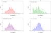 |
Fig. 7 The distribution of SMBH masses for both normal (white) and AGN (colored) host galaxies as a function of morphology (Δ [log 10M• ] = 0.05 bin). The data of the galaxies have been extracted from the Sloan Digital Sky Survey in redshift interval 0.02 < z < 0.05. The masses have been inferred via the M• − σ relation using the slope and the normalization taken from Table 2. In order to compare our results with that of Schawinski et al. (2010), we plotted only objects where the measured velocity dispersion is greater than 40 km s-1. |
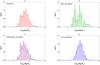 |
Fig. 8 The distribution of SMBH masses for both normal (white) and AGN (colored) host galaxies as a function of morphology (Δ [log 10M• ] = 0.05 bin). The data of the galaxies have been extracted from the Sloan Digital Sky Survey in redshift interval 0.02 < z < 0.05. The masses have been inferred from the kinetic energy of random motions via the M• − Mdynσ2 relation using the slope and the normalization taken from Table 2. In order to compare our results with that of Schawinski et al. (2010), we plotted only objects where the measured velocity dispersion is greater than 40 km s-1. |
Actually, a similar double-peak figure has been found by Capetti & Balmaverde (2006) plotting the distributions of radio-quiet and radio-loud AGN galaxies selected from the HST and Chandra archival data. So the double peak in the early-type AGN (Fig. 8b) could be easily explained by the radio-quiet/radio-loud dichotomy.
As already noted by Chiaberge et al. (2005), all radio-loud AGN are associated with SMBH masses ≳ 108 M⊙, whereas most of the radio-quiet population has lower SMBH masses. A similar result has been recently found by Baldi & Capetti (2010) and Chiaberge & Marconi (2011), and is in agreement with what we found in Fig. 8b. Since radio-galaxies are almost universally found hosted by elliptical galaxies (Urry & Padovani 1995), this explains why we did not see any double peak in the late-type AGN galaxies (Fig. 8d).
It would be interesting to examine a larger sample of AGN in order to understand if this double peak is real or caused by a too small sampling, but this is beyond the scope of this paper. What we want to show here is that if we use the M• − Mdynσ2 instead of the M• − σ relation, we obtain different SMBH mass distributions (compare Figs. 7 with 8). Consequently it is better not to go on easy conclusions regarding the activity and the evolution of both AGN and normal host galaxies, until we have understood what the best scaling law able to infer correctly the SMBH masses is.
6. Conclusion
We analyzed different scaling laws for a consistent sample formed by N = 52 galaxies, which have been catalogued by Sani et al. (2011) on the base of Spitzer/IRAC 3.6 μm observations of local Universe. The sample is formed by both early-type and late-type galaxies. Actually, from the original sample of 57 galaxies, we removed 5 disc galaxies identified by Sani et al. (2011) as hosting pseudobulges and that are non consistent with the correlations for classical bulges. For the galaxy masses, we considered both the dynamical mass and the stellar mass. The results of our analysis have been reported in Table 2, and Figs. 1 − 4.
The main emerging result is that the relation between the mass of SMBHs and the kinetic energy of random motions of the host local galaxies appears to be a robust correlation, which could provide the right passkey to understand the nature and evolution of the numerous observed correlations between SMBHs and host spheroid properties. This is in agreement with our previous studies performed on the samples of Graham (2008a), Gültekin et al. (2009a), and Hu (2009). Even if the values of the  (see Table 2) indicate that the M• − MGσ2 works better than the others, by considering the intrinsic scatter of the various relations and in particular their errors, we cannot conclusively determine the best relation, because all the examined laws appear on the same level. The comprehensive analysis of residuals discussed in Sect. 4 does not confirm the result claimed by Hopkins et al. (2007b), according to which a black hole FP should be preferred over a simple one-one relation, even if it cannot be definitively ruled out.
Since it has now been tested on four different samples of galaxies, independently catalogued by different authors, the goodness of the M• − MGσ2 relation as a predictor of the SMBH mass in the center of galaxies is enough robust. Again, this relation is the only one that currently has a quite clear physical explanation. In this perspective, as we discussed in Sect. 5, in order to obtain correct estimates of SMBH masses, the M• − MGσ2 relation should be preferably used instead of the other popular scaling laws. As a matter of fact, the SMBH mass distribution of the early-type AGN galaxies, inferred by a much more physically motivated relation, clearly shows the radio-quiest/radio-loud dichotomy. The same result is not achieved if we use the usual M• − σ relation.
Here we use the terms bulge or spheroid to mean the spheroidal component of a spiral/lenticular galaxy or a full elliptical galaxy.
Essentially, a pseudobulge is a bulge that shows photometric and kinematic evidence for disk-like dynamics (Kormendy 1993).
Another effort in this sense has been performed by Gültekin et al. (2009b), who analyzed the relationship among X-ray luminosity, radio luminosity, and mass of a sample of SMBHs, identifying a FP that can be turned into an effective SMBH mass predictor.
www.galaxyzoo.org
Acknowledgments
We wish to thank Roberto De Carli, Alister Graham, Alessandro Marconi, Nikolay Nikolov, Eleonora Sani, Kevin Schawinski for their useful suggestions and private communications. We also thank the referee for many suggestions that have helped us to improve our paper considerably. L.M. thanks the Harvard Smithsonian Center for Astrophysics for the kind hospitality, and acknowledges support for this work by research funds of the University of Sannio, and the International Institute for Advanced Scientific Studies.
References
- Aller, M. C., & Richstone, D. O. 2007, ApJ, 665, 120 [NASA ADS] [CrossRef] [Google Scholar]
- Baes, M., Buyle, P., Hau, G. K. T., & Dejonghe, H. 2003, MNRAS, 341, L44 [NASA ADS] [CrossRef] [Google Scholar]
- Baldi, R. D., & Capetti, A. 2010, A&A, 519, A48 [NASA ADS] [CrossRef] [EDP Sciences] [Google Scholar]
- Beifiori, A., Sarzi, M., Corsini, E. M., et al. 2009, ApJ, 692, 856 [NASA ADS] [CrossRef] [Google Scholar]
- Beifiori, A., Courteau, S., Corsini, E. M., & Zhu, Y. 2011, MNRAS, in press [arXiv:1109.6265] [Google Scholar]
- Bellovary, J., Volonteri, M., Governato, F., et al. 2011, ApJ, 742, 13 [NASA ADS] [CrossRef] [Google Scholar]
- Bower, R. G., Benson, A. J., Malbon, R., et al. 2006, MNRAS, 370, 645 [NASA ADS] [CrossRef] [Google Scholar]
- Burkert, A., & Tremaine, S. 2010, ApJ, 720, 516 [NASA ADS] [CrossRef] [Google Scholar]
- Capetti, A., & Balmaverde, B. 2006, A&A, 453, 27 [NASA ADS] [CrossRef] [EDP Sciences] [Google Scholar]
- Cappellari, M., Bacon, R., Bureau, M., et al. 2006, MNRAS, 366, 1126 [NASA ADS] [CrossRef] [Google Scholar]
- Chiaberge, M., & Marconi, A. 2011, MNRAS, 416, 917 [NASA ADS] [CrossRef] [Google Scholar]
- Chiaberge, M., Capetti, A., & Macchetto, F. D. 2005, ApJ, 625, 716 [NASA ADS] [CrossRef] [Google Scholar]
- De Lucia, G., & Blaizot, J. 2007, MNRAS, 375, 2 [NASA ADS] [CrossRef] [Google Scholar]
- Feoli, A., & Mele, D. 2005, Int. Jour. Mod. Phys. D, 14, 1861 [Google Scholar]
- Feoli, A., & Mele, D. 2007, Int. Jour. Mod. Phys. D, 16, 1261 [Google Scholar]
- Feoli, A., & Mancini, L. 2009, ApJ, 703, 1502 [NASA ADS] [CrossRef] [Google Scholar]
- Feoli, A., & Mancini, L. 2011, Int. Jour. Mod. Phys. D, in press [arXiv:1012.3160] [Google Scholar]
- Feoli, A., Mancini, L., Marulli, F., & van den Bergh, S. 2011, Gen. Rel. Grav., 43, 1007 [NASA ADS] [CrossRef] [Google Scholar]
- Ferrarese, L. 2002, ApJ, 578, 90 [NASA ADS] [CrossRef] [Google Scholar]
- Ferrarese, L., & Merritt, D. 2000, ApJ, 539, L9 [NASA ADS] [CrossRef] [Google Scholar]
- Gebhardt, K., Bender, R., Bower, G., et al. 2000, ApJ, 539, 13 [Google Scholar]
- Gebhardt, K., Richstone, D. O., Tremaine, S., et al. 2003, ApJ, 583, 92 [NASA ADS] [CrossRef] [Google Scholar]
- Graham, A. W. 2008a, PASA, 25, 167 [NASA ADS] [CrossRef] [Google Scholar]
- Graham, A. W. 2008b, ApJ, 680, 143 [NASA ADS] [CrossRef] [Google Scholar]
- Graham, A. W. 2011 [arXiv:1103.0525] [Google Scholar]
- Graham, A. W., & Driver, S. P. 2005, PASA, 22, 118 [NASA ADS] [CrossRef] [Google Scholar]
- Graham, A. W., & Driver, S. P. 2007, ApJ, 655, 77 [NASA ADS] [CrossRef] [Google Scholar]
- Graham, A. W., Onken, C. A., Athanassoula, E., & Combes, F. 2011, MNRAS, 412, 2211 [NASA ADS] [CrossRef] [Google Scholar]
- Gültekin, K., Cackett, E. M., Miller, J. M., et al. 2009a, ApJ, 698, 198 [NASA ADS] [CrossRef] [Google Scholar]
- Gültekin, K., Cackett, E. M., Miller, J. M., et al. 2009b, ApJ, 706, 404 [NASA ADS] [CrossRef] [Google Scholar]
- Häring, N., & Rix, H. 2004, ApJ, 604, L89 [NASA ADS] [CrossRef] [Google Scholar]
- Ho, L. C. 2004, Coevolution of Black Holes and Galaxies (Cambridge Univ. Press), Carnegie Observatories Astrophys. Ser., 1 [Google Scholar]
- Hopkins, P. F. 2008, in Formation and Evolution of Galaxy Bulges, ed. M. Bureau, E. Athanassoula, & B. Barbuy (Cambridge: Cambridge Univ. Press), IAU Symp., 245, 219 [Google Scholar]
- Hopkins, P. F., Hernquist, L., Cox, T. J., et al. 2007a, ApJ, 669, 45 [NASA ADS] [CrossRef] [Google Scholar]
- Hopkins, P. F., Hernquist, L., Cox, T. J., et al. 2007b, ApJ, 669, 67 [NASA ADS] [CrossRef] [Google Scholar]
- Hu, J. 2008, MNRAS, 386, 2242 [NASA ADS] [CrossRef] [Google Scholar]
- Hu, J. 2009, MNRAS, submitted [arXiv:0908.2028] [Google Scholar]
- Jahnke, K., & Macciò, A. 2011, ApJ, 734, 92 [NASA ADS] [CrossRef] [Google Scholar]
- Kelly, B. C. 2007, ApJ, 665, 1489 [NASA ADS] [CrossRef] [Google Scholar]
- Kisaka, S., Kojima, Y., & Otani, Y. 2008, MNRAS, 390, 814 [NASA ADS] [CrossRef] [Google Scholar]
- Kormendy, J. 1993, in Galactic Bulges, ed. H. DeJonghe, & H. Habbing (Dordrecht: Kluwer), IAU Symp., 153, 209 [Google Scholar]
- Kormendy, J., & Bender, R. 2011, Nature, 469, 377 [NASA ADS] [CrossRef] [PubMed] [Google Scholar]
- Kormendy, J., & Richstone, D. 1995, ARA&A, 33, 581 [NASA ADS] [CrossRef] [Google Scholar]
- Laor, A. 2001, ApJ, 553, 677 [NASA ADS] [CrossRef] [Google Scholar]
- Lauer, T. R., Faber, S. M., Richstone, D., et al. 2007, ApJ, 662, 808 [NASA ADS] [CrossRef] [Google Scholar]
- Marulli, F., Bonoli, S., Branchini, E., et al. 2008, MNRAS, 385, 1846 [NASA ADS] [CrossRef] [Google Scholar]
- Magorrian, J., Tremaine, S., Richstone, D., et al. 1998, AJ, 115, 2285 [NASA ADS] [CrossRef] [Google Scholar]
- Marconi, A., & Hunt, L. K. 2003, ApJ, 589, L21 [NASA ADS] [CrossRef] [Google Scholar]
- Merritt, D., & Ferrarese, L. 2001, ApJ, 547, 140 [NASA ADS] [CrossRef] [Google Scholar]
- Novak, G. S., Faber, S. M., & Dekel, A. 2006, ApJ, 637, 96 [NASA ADS] [CrossRef] [Google Scholar]
- Press, W. H., Teukolsky, S. A., Vetterling, W. T., & Flannery, B. P. 1992, Numerical Recipes, 2nd edn. (Cambridge: Cambridge University Press) [Google Scholar]
- Richstone, D., Ajhar, E. A., Bender, R., et al. 1998, Nature, 395, A14 [NASA ADS] [Google Scholar]
- Sani, E., Marconi, A., Hunt, L. K., & Risaliti, G. 2011, MNRAS, 413, 1479 [NASA ADS] [CrossRef] [Google Scholar]
- Schawinski, K., Urry, C. M., Virani, S., et al. 2010, ApJ, 711, 284 [NASA ADS] [CrossRef] [Google Scholar]
- Schneider, P. 2006, Extragalactic astronomy and cosmology (Berlin Heidelberg: Springer-Verlag) [Google Scholar]
- Snyder, G. F., Hopkins, P. F., & Hernquist, L. 2011, ApJ, 728, L24 [NASA ADS] [CrossRef] [Google Scholar]
- Soker, N., & Meiron, Y. 2011, MNRAS, 411, 1803 [NASA ADS] [CrossRef] [Google Scholar]
- Strauss, M. A., Michael, A., Weinberg, D. H., et al. 2002, AJ, 124, 1810 [NASA ADS] [CrossRef] [Google Scholar]
- Tremaine, S., Gebhardt, K., Bender, R., et al. 2002, ApJ, 574, 740 [NASA ADS] [CrossRef] [Google Scholar]
- Urry, C. M., & Padovani, P. 2011, PASP, 107, 803 [Google Scholar]
- Volonteri, M., Natarajan, P., & Gultekin, K. 2011, ApJ, 737, 50 [NASA ADS] [CrossRef] [Google Scholar]
- Wandel, A. 2002, ApJ, 565, 762 [NASA ADS] [CrossRef] [Google Scholar]
All Tables
The values of the stellar mass and 1σ error for each galaxy of the sample (Sani & Marconi 2011, priv. comm.).
Regression results for log M• = b + mlog x with a sample composed by 52 galaxies.
All Figures
|
Fig. 1 M• − Mdynσ2 (left) and M• − M ⋆ σ2 (right) relations for the sample of N = 52 galaxies extracted from the data set of Sani et al. (2011). The symbols represent elliptical galaxies (red ellipses), lenticular galaxies (green circles), barred lenticular galaxies (dark green circles), spiral galaxies (blue spirals), barred spiral galaxies (dark blue barred spirals), and dwarf elliptical galaxies (orange ellipses). The black lines are the lines of best fit. |
| In the text | |
|
Fig. 2 M• − Mdyn (left) and M• − M ⋆ (right) relations for the sample of N = 52 galaxies extracted from the data set of Sani et al. (2011). The symbols are the same as in Fig. 1. |
| In the text | |
|
Fig. 3 M• − σ200 (left) and M• − Reσ3 (right) relations for the sample of N = 52 galaxies extracted from the data set of Sani et al. (2011). The symbols are the same as in Fig. 1. |
| In the text | |
|
Fig. 4 M• − Mdynσ (left) and M• − M ⋆ σ (right) relations for the sample of N = 52 galaxies extracted from the data set of Sani et al. (2011). The symbols are the same as in Fig. 1. |
| In the text | |
|
Fig. 5 Residuals of M• − σ as a function of the host galaxy effective radius Re (left) and stellar mass M ⋆ (right), for the full sample of 57 galaxies (a − b), and for a more consistent sample (see text) of 52 galaxies (c–d), respectively. The corresponding intrinsic scatter and Pearson linear coefficient are reported in the upper-left corner of each plot. The symbols are the same as in Fig. 1. Galaxies inside the black circles are pseudo-bulges. |
| In the text | |
|
Fig. 6 Correlations between the residuals in the M• − σ and Re − σ (left), and M ⋆ − σ (right) relations at each σ (Hopkins et al. 2007b), for the full sample of 57 galaxies (a–b), and for a more consistent sample (see text) of 52 galaxies (b–c). The corresponding intrinsic scatter and Pearson linear coefficient are reported in the upper-left corner of each plot. The symbols are the same as in Fig. 1. Galaxies inside the black circles are pseudo-bulges. |
| In the text | |
|
Fig. 7 The distribution of SMBH masses for both normal (white) and AGN (colored) host galaxies as a function of morphology (Δ [log 10M• ] = 0.05 bin). The data of the galaxies have been extracted from the Sloan Digital Sky Survey in redshift interval 0.02 < z < 0.05. The masses have been inferred via the M• − σ relation using the slope and the normalization taken from Table 2. In order to compare our results with that of Schawinski et al. (2010), we plotted only objects where the measured velocity dispersion is greater than 40 km s-1. |
| In the text | |
|
Fig. 8 The distribution of SMBH masses for both normal (white) and AGN (colored) host galaxies as a function of morphology (Δ [log 10M• ] = 0.05 bin). The data of the galaxies have been extracted from the Sloan Digital Sky Survey in redshift interval 0.02 < z < 0.05. The masses have been inferred from the kinetic energy of random motions via the M• − Mdynσ2 relation using the slope and the normalization taken from Table 2. In order to compare our results with that of Schawinski et al. (2010), we plotted only objects where the measured velocity dispersion is greater than 40 km s-1. |
| In the text | |
Current usage metrics show cumulative count of Article Views (full-text article views including HTML views, PDF and ePub downloads, according to the available data) and Abstracts Views on Vision4Press platform.
Data correspond to usage on the plateform after 2015. The current usage metrics is available 48-96 hours after online publication and is updated daily on week days.
Initial download of the metrics may take a while.