| Issue |
A&A
Volume 536, December 2011
|
|
|---|---|---|
| Article Number | A57 | |
| Number of page(s) | 16 | |
| Section | Planets and planetary systems | |
| DOI | https://doi.org/10.1051/0004-6361/201014862 | |
| Published online | 07 December 2011 | |
Effects of the planetary migration on some primordial satellites of the outer planets⋆
I. Uranus’ case
1 Universidade Estadual Paulista, IGCE-DEMAC, Caixa Postal 178, CEP 13.500-970 Rio Claro (São Paulo), Brasil
e-mail: This email address is being protected from spambots. You need JavaScript enabled to view it.
; This email address is being protected from spambots. You need JavaScript enabled to view it.
2
Observatório Nacional, Rua General Cristino 77, CEP 20921-400 Rio de Janeiro, RJ, Brasil
3 Universidade de São Paulo, IAG-USP, Rua do Matão 1226, CEP 05508-090, Cidade Universitária, São Paulo, Brasil
Received: 25 April 2010
Accepted: 12 September 2011
Abstract
Context. During the first hundred million years after the formation of our solar system, the four giant planets are believed to have migrated significantly (by up ≈ 20 AU). The current scenario and dynamics of the satellites of these planets must be the result of both the initial conditions of their formation and this early extensive migrational episode.
Aims. We examine the effects of the migration on the primordial satellites of Uranus.
Methods. We use the Nice model to generate templates for the evolution of the four giant planets and record the time history of these planets and important close encounters. The satellites are then added to Uranus and these objects are integrated according to the dynamics stored in the templates.
Results. We show that Oberon is the outermost regular satellite of Uranus that is able to resist the close encounters during the extensive migrational episode. Some theories predict that Uranus’ satellites can form out to a 57 RU distance from the planet, but we show that even those at ≈ 27 RU from the planet cannot support the instabilities that appeared during migration. Close objects, such as the current regular satellites of Uranus, can survive quite stably and we are able to place some constraints on the masses of the planetesimals that have close encounters. For instance, if an object with mass ≥ 10-9 M⊙ approaches at distances ≲ 23 RU from Uranus, the regular satellites can be destabilized or their eccentricities or inclinations excited to some non-compatibles values. We also find that planet-planetesimal close encounters can generate capture. In this way, we present a promising means of explaining the origin of the irregular satellites of Uranus. The importance of the oblateness of the planet, and the Sun for just-captured planetesimals is also shown.
Key words: celestial mechanics / planets and satellites: general / planets and satellites: individual: Uranus
Appendix B is available in electronic form at http://www.aanda.org
© ESO, 2011
1. Introduction
It is widely believed that the original distances of the giant planets (with respect to the Sun) as soon as the circumsolar gaseous nebula had dissipated, experienced significant changes due to the phenomenon of migration (Fernandez & Ip 1996; Malhotra 1993; Hahn & Malhotra 1999; Tsiganis et al. 2005, etc.). Very roughly speaking, in the migrational process, the interaction between the protoplanets and the planetesimals during the early stage of the solar system, caused significant displacements in the primordial configuration of these planets. Some different migrational scenarios have been presented, although it seems that, the Nice model is the most accepted and capable to reproducing our current solar system. The original Nice model (Tsiganis et al. 2005) was subsequently revised (Morbidelli et al. 2007; Brasser et al. 2009), although its basic principles remain preserved. For more details, we refer to a review in Morbidelli et al. (2010).
Once a migrational framework is established, it is perhaps more important than studying migration itself, to devote our attention to the dynamics of the other bodies that suffered the direct consequences of the displacement of the giant planets. Following Fernandez & Ip (1996), many papers about, for instance, Trojans, asteroids, Plutinos, and KBOs, have appeared. However, as mentioned in Nesvorný et al. (2007), in our race to understand, at least part of the evolutionary history of our system, the population of the satellites occupies a position of major interest. According to these authors, the study of the satellites can provide information that cannot be obtained from any other source. Since it is believed that distant satellites (in contrast to those called regular) are captured objects, these authors give in the introduction of their paper, an interesting and precise discussion of the several theories on the capture of the distant satellites. The basic ideas of each theory are highlighted and possible drawbacks are discussed. In the main body of their article, they present their new theory of capture based on planetary close encounters that happen in the Nice migrational model. While most investigations have been devoted to distant satellites, we also include in our study the possible effects of migration on certain primordial satellites that formed close to the planet. We also consider whether possible satellites beyond Oberon, Callisto, or Hyperion could withstand the close encounters that occurred during migration or if no object existed at these distances. It is usually accepted that inner (or regular) satellites were immune to migrational phenomena, but as far we are aware, no direct investigation of this problem has yet been presented. We clearly need to determine the distance from the mother planet at which a regular satellite can resist the migrational phenomenon. In this first paper, we try to focus our attention on Uranus’ satellites. This work is organized in the following way. In Sect. 2, we adopt the definition of critical distance ac by Goldreich (1966) to classify regular and irregular satellites. In Sect. 3, we present some migrational models. Section 4 illustrates the extreme sensitivity of these models to an object that is inserted into the integration of the planets. In Sect. 4, to avoid this sensitivity problem, we propose our interpolator technique. Section 5 shows the results of the numerical simulations considering Uranus and its satellites. Oberon resists the close encounters, while other fictitious satellites beyond it are destabilized. As a by-product of several close encounters, some planetesimals can be captured by Uranus and these objects are candidates of irregular satellites as seen today. Section 6 presents some of these captures. Section 7 is devoted to conclusions. In Appendix A, we show the importance of the oblateness and the effect of the Sun on the dynamics of the satellites. We also included some supplementary tables and figures in Appendix B.
2. Regular and irregular satellites
Various studies of planetary migration (Fernández & Ip 1996; Hahn & Malhotra 1999; Tsiganis et al. 2005, etc.) have triggered many investigations of planetary satellites, in particular those more distant from the planet (“irregular”), because according to some authors, those close to the planets (“regular”) are almost unaffected by migrational phenomenon.
A detailed study of this insensitivity certainly requires a non-negligible cpu-time because the orbital period of these satellites are much shorter than the period of those so-called “irregular” satellites (Callegari & Yokoyama 2008). Moreover, this kind of insensitivity must consider not only the current “regular” satellites, but also the stability of others beyond the outermost current satellite according to what we understand by a “regular” satellite. It is clearly expected that the closer the satellite, the tighter the link to the planet. Tsiganis et al. (2005), Nesvorný et al. (2007), and others, found that the regular satellites undergo only minor perturbations during the planetary close encounters. The name “regular” satellite, in general, is given to those very close to the planet of small eccentricity and inclination. Those far from the planet, usually with significant eccentricity and inclination, are called irregular. With some exceptions (Triton and possibly Nereid, Phoebe, or Iapetus), this classification expresses the different origins of each group: the former are supposed to be primordial, more precisely, neglecting tidal effects, they were formed “in situ” while the second group originated from captured objects.
Instead of this qualitative definition, an alternative and perhaps more accurate classification can be made following Goldreich (1966) and Burns (1986). We first consider the so-called critical semi-major distance  (1)where J2, Mp, ap, and ep are the oblateness coefficient, mass, semi-major axis, and eccentricity of the planet, and M⊙ refers to the mass of the Sun.
At this distance, the torque on the orbit of the satellite caused by the oblateness is equal to the torque produced by the Sun. A simple calculation shows that for objects with semi-major axis a < ac the inclination remains almost constant with respect to the equator, while for a > ac the object maintains a constant inclination with respect to the orbital plane of the planet, not to the equator. For distances close to ac and depending on the obliquity of the planet, the eccentricity and the motion of the satellite, in general, can become very irregular (Yokoyama 2002).
It is well accepted that the close satellites were formed from circumplanetary material in a disk about the planet. In particular, the only plane where a disk of particles can remain without dispersing, is the equatorial plane (Goldreich 1966). On the other hand, this disk must be confined to a region within ac. Therefore, again following Goldreich (1989), equatorial satellites with semi-major axes smaller than ac reflect a condition of origin, not evolution.
On the basis of these arguments, it is little wonder that almost all the known satellites called “regular”, are within ac. Almost all of them are prograde of very small eccentricity and inclination. The exception is Triton.
In Table 1, we list the critical semi-major axis of the giant planets. The first column gives ac for the current configuration and the values of the current semi-major axis of the planets are given on the right within parentheses. The second column is similar but the values within the parentheses are the semi-major axes of the planets inferred by Tsiganis et al. (2005). In the last column, we give the outermost known satellite within ac. Its distance (in Rp) from the planet is also given within brackets.
It is interestint to note that all the satellites whose semi-major axes are larger than ac given in Table 1, have either a large eccentricity or significant inclination relative to those with a < ac. Hence, for the sake of clarity in the nomenclature in this work, we refer to as “regular” those satellites whose semi-major axes are within ac, and otherwise we refer to a satellite as “irregular”.
For Uranus, we can see an interesting gap: in spite of a very large ac, the outermost satellite Oberon is only 22.8 RU away from Uranus. No satellite currently exists in the large interval [22.8 RU, ac]. Compared to Jupiter and Saturn, this difference seems to be quite large.
At first sight, it seems that there is a lack of satellites at larger radii than Oberon. The absence of these satellites indicates that they were either depleted during the close encounters during migration or never existed. For Neptune, this lack of satellites seems to be even more crucial, although the situation seems to be different and more complicated owing to the possible capture of Triton in the past and that the unusual orbit of Nereid should be taken into account conplicating the whole dynamics considerably (Goldreich et al. 1966; Cúk & Gladman 2005; Agnor & Hamilton 2006).
In the same way, we note the large distance that the current irregular satellites keep from the critical semi-major axis ac of the correspondent planet. For instance, in the case of Jupiter, the nearest irregular satellite is about 80 RJ away from Callisto (Jewitt & Haghighipour 2007). Perhaps this large distance is associated with collisions (Bottke et al. 2010) between the outermost regular satellite (Callisto in the case of Jupiter) with highly eccentric and irregular captured satellites. Usually the masses of irregular satellites (captured objects) are much lower than the masses of the outermost regular satellites. In this situation, a collision causes either the destruction or ejection of those of low mass.
The question of why Oberon, Hyperion, and Callisto are the outermost regular satellites observed today, may certainly have the answer that their orbtis are the product of many complex events in the past. These events are related to the satellite formation process (Mosqueira & Estrada 2003; Canup & Ward 2000, 2006), planetary migration (including collisions), and dynamical instability. In particular for Uranus, we propose that the results on migrational theory of Tsiganis et al. (2005) can provide interesting results in this direction. This study also permits us to test the Nice model, since the overall network of the satellites (not only the irregular ones) should have been influenced by the planetary migration.
3. Migrational models
Here we consider the Nice model, or more precisely Gomes’ code (Gomes et al. 2005). Morbidelli et al. (2007) presented a second version of the Nice model (Nice-II). Although in the original model (Nice-I), the initial conditions of the four giant planets are rather arbitrary, in Nice-II the initial conditions of the giant planets are defined as a result of an hydrodynamical simulation related to the evolution of the planets in a gaseous proto-planetary disk. In this way, the planets begin their migration in a compact quadruple resonant configuration, that is, Jupiter and Saturn are in 3S:2J mean motion resonance, Uranus and Saturn in 3U:2S, and Uranus and Neptune in 4N:3U. The main source of the instability during the migration is the crossing of the Jupiter-Saturn 5S:3J resonance, although later the crossing of the 2S:1J resonance also occurs, which is much faster than in the Nice-I version.
In the Nice-I model, if migration of the giant planets occurred after the completion of the inner planets, it is clear that the terrestrial planets suffered a violent bombardment (LHB phenomenon). While the current configuration of the giant planets is well reproduced by this model, it is also important to check how the inner planets supported the effects of migration and to explore establish whether the current configuration of the terrestrial planets is compatible with the migration theory.
To explain the current architecture of the inner planets in the context of the migration theory, Brasser et al. (2009) switched from the Nice-I to the Nice-II model, since a slow passage through 2:1 Jupiter-Saturn resonance that occurs in Nice-I, could give birth to some undesirable secular resonances causing incompatible eccentricities in the terrestrial planets. As mentioned in Brasser et al. (2009), the two models differ only in some technical details, although the bulk of the dynamics (global instability caused by the passage of Jupiter-Saturn pair through a mean-motion resonance and a later stabilization owing to the dynamical friction) remain the same.
Although the original Nice-I model might not be adequate to reconcile the current status of the terrestrial planets and the LHB history (provoked by this migration theory), it has been tested in several scenarios, reproducing many observational aspects of our solar system (Morbidelli et al. 2005; Nesvorný et al. 2007; Gomes et al. 2005). Therefore, we consider only Nice-I in this work, for which the important ingredient is the strong bombardment of the planetesimals on the planets related to some violent close encounters between the planets. As mentioned in Morbidelli et al. (2009a), the migration of the planets cannot be smooth. For instance, if smooth migration is accepted, in the case of Uranus we can show the appearance of some captures in resonances for the regular satellites. These resonances would be responsible for some non-realistic increase in the inclinations of the satellites, especially for Umbriel (Yokoyama, in prep.).
After several experiments considering different initial positions of the planets and sufficient time integration (109,6 × 10⁸ years), we selected five cases that we call M1, M2, M3, M4, and M5. The time evolution of the planets is shown in Fig. 1. We show only the first 5 or 10 Myr, i.e., a short interval around the region where the 2S:1J resonance occurs and some planetary close encounters as well. At the end of this short time interval, the eccentricity and inclination of the planets are still larger than the current values. However, in general, once the planets acquire these kinds of configuration, no more planetary close approaches will occur and the semi-major axes will usually remain almost constant, as the eccentricity and inclination are damped very slowly to their current values by the dynamical friction. This usually takes about 100 Myr.
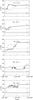 |
Fig. 1 Models Mi: time evolution of the semi-major axes of the planets during the passage through 2S:1J resonance. |
Following Gomes et al. (2005), the total mass of the planetesimal disk is 35 M ⊕ (where M ⊕ refers to Earth’s mass). In the beginning, this disk is represented by only a few hundred objects (500), such that the mass of each particle is about ≈ 2.1 × 10⁻⁷ M⊙. During the time evolution, whenever this particle approaches within a distance of DP of some planet (DP ≈ 3 AU), the planetesimal is substituted by 20 new particles, which are randomly distributed within a circle of radius ≈ 0.01 AU centered on the original planetesimal. In this process, the mass of the parent planetesimal is equally partitioned among the new particles ( ≈ 1.05 × 10⁻⁸ M⊙). Every 10 000 years, the code verifies the planet-planetesimal distance and for all close approaches ≤ DP, the above technique is applied, although planetesimals that originated from a previous partition are not allowed to be cloned again. The main idea of this process is just to define the optimal number of particles with suitable values of individual mass, such that the cpu-time of the integration is acceptable while migration as a whole, is sufficiently smooth without exhibiting too strong noise in the variation of the elements. After these partitions, we usually worked with a total of Npmax ≤ 10 000 particles. This is the effective planetesimal disk that governs the scenario of the migration. The five successful models, previously mentioned, were obtained considering this disk of planetesimals.
4. Methodology
We propose to study the stability of the regular satellites and fictitious objects near the outermost inner satellite of Uranus considering the effects of migration theory based on Nice-I model. To do that, we basically define two steps. In the first, we collect a number of successful migrations scenarios (five simulations) and during the integration of the four planets we record at each seven years, the position and velocity of the planets. To test the effect of migration on the primordial satellites, we have of course, to consider only successful simulations. A naive way of studying the dynamics of the planetary satellites is to re-run a successful migration model, but now including the satellites of the mother planets. In doing this, we note that the results are very sensitive to very small changes in the numerical integration of the system. The inclusion of a small satellite (even with almost zero mass) in the integrations, may cause large enough changes that the previous successful configuration of the outer planets cannot be reproduced anymore. As the system is strongly chaotic during the passage through the 2S:1J resonance, Uranus and Neptune may follow different paths and a small perturbation can generate important consequences, including the escape of either Neptune or Uranus. For instance, taking one simulation among the preceding simulations, keeping the same initial conditions, same machine and just adding some more satellites, the final result of the integration can completely change as shown in Fig. 2. The top panel of this figure exhibits the evolution of the planets when three satellites of Uranus, at distances 25 RU, 40 RU, and 55 RU are included in migrational model. In the bottom panel of Fig. 2, we included two satellites at 30 RU and 60 RU. We note that the behavior of the ice-planets is quite different. In particular, for the top panel, as Uranus has some close encounters with Jupiter, the three satellites are ejected in about 6 × 10⁵ years. In general, there is no guarantee that the final solar system will be recovered whenever an extra object, such as a regular satellite, is included in the system. In some cases, we can have the escape of Neptune or Uranus. In both cases, the Burlirsh-Stoer (BS2) integrator of the Mercury package was used (Chambers 1999).
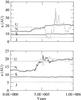 |
Fig. 2 Top: three satellites of Uranus (a = 25 RU, a = 40 RU, a = 55 RU) are included in a previous simulation. Bottom: same as on the top, including only two satellites: (a = 30 RU, a = 60 RU). The path of the ice planets changes completely with the inclusion of these satellites. |
Therefore, owing to this high sensitivity, the inclusion of target objects in a previous successful migration is not viable. In addition to this problem, the simulation of a migrational model can be very time-consuming, especially when close satellites are included.
To overcome these problems, we consider migrational models whose final outcomes reproduced our current solar system. Our technique is to use these models as fixed templates and insert the target satellites to be studied under the action of the migrating planets and also under the effect of some “selected” planetesimals. The meaning of “selected” will be explained later. The method of avoiding the high sensitivity was presented in Yokoyama et al. (2009) and also in Brasser et al. (2009).
To derive the template for each successful migration, the heliocentric orbital elements (a, e, I, Ω, ω) of the four giant planets are recorded to build a discrete database of the complete time evolution of the planets. We usually record these elements every seven years. With this database for every three points, an interpolating quadratic polynomial in time can be defined to represent the semi-major axis, eccentricity, inclination, longitude of the node, and argument of the pericenter for each planet. Every 14 years, except for the mean anomaly, a new polynomial is constructed for each orbital element of the planets. We note that once the semi-major axis is fitted using a polynomial, the corresponding mean anomaly can be triavilly found from the two-body problem approximation. With this technique the motion of the migrating planets is given for any time and test satellites can be inserted in this system with the guarantee that the planets will reproduce the previous successful path. Once the template is obtained, any set of new satellites can be inserted and we can run the same code because only the satellites are integrated, that is, the orbits of the planets are supplied by the polynomials of the template.
During the planetary migration, several close encounters between planets and planetesimals occur. Our code checks this planet-planetesimal distance every 14 years. We define as t = t∗ the instant when a close approach between Uranus and a planetesimal occurs, such that the separation distance is ≤ 0.8 AU (Beaugé et al. 2002; Nesvorný et al. 2007; Nogueira 2008). Starting from t = t∗, the planet-planetesimal system is integrated backward until t = t∗∗, when the separation distance becomes greater than 1.0 AU. This is a simple two-body problem integration whose origin is fixed on the equator of the planet. In this case, the integrator is switched to Radau with a very short time-step (of the order of one day). From t = t∗∗, a forward integration is then carried out and if the planetesimal approaches within 100 RU of the planet (at t = t∗∗∗) we record its planetocentric position and velocity. These are the “selected” planetesimals we mentioned before and are processed later (in a second step), considering a more complete environment that includes the Sun, oblateness, the remaining planets, and the regular satellites. As the time step is very short, usually at t = t∗∗∗ the distance between “selected” planetesimal and Uranus is very close to 100 RU. We later consider other distances (200 RU and 300 RU).
In the Nice model, we recall that we considered a disk with 35 M⊕ represented by at most ten thousand particles. This means that the individual mass is about 1.05 × 10⁻⁸ M⊙. A very large number of planetesimals means lower individual masses for them and of course, a smooth migrational process, although a much longer cpu-time is needed to simulate the migration.
While the disk that we use is reasonable for simulating successfully the migration of the planets, it is clear that for the dynamics of the satellites, the masses of these planetesimals are too large relative to the masses of Miranda, Umbriel and other groups (see Sect. 5). If the mass of the planetesimals were on the order of 1.05 × 10⁻⁸ M⊙, it would be difficult to explain the current mass distribution of bodies in the Kuiper belt and also the current irregular satellites. In addition, the survival of the regular satellites in their current orbits would be very unlikely. One could say that eventually, some so large planetesimal might have existed in the disk, although the majority of them could not have had high masses. In the next subsection, we discuss the question of the masses.
4.1. Close encounters and mass of the planetesimals
The dynamics of the satellites during migration involves the interaction of the host planet with the remaining planets as well as the effects of the “selected” planetesimals on these satellites. As mentioned before, with the interpolating technique, the computation of the effects of the planets becomes easy, although the effects of the planetesimals on the satellites must be worked out independently.
In addition to the perturbations due to the planets and the oblateness, we assume that what really does matter is the effect that occurs when the pair satellite-planetesimal is in a close encounter geometry. Unless the planetesimal approaches the planet very closely we consider that its effect on the satellites is negligible. This is somehow straightforward considering the masses of the participants.
To take into account the close approach, we have to set a value for the mass of each planetesimal that approaches the planet. According to Trujillo et al. (2001), the cumulative distribution number (N) of particles with radius r, belonging to the Kuiper belt follows a power law N ∝ r − q (q = 4 ± 0.5). For asteroids of the main belt, the value q ≈ 3.5 (Jewitt & Haghighipour 2007), may vary significantly. For Jovian irregular satellites, it seems that a single power law cannot perfectly describe the current distribution. The unknown process of evolution of the satellites (dynamics, collision, re-accumulation, etc.) might have perturbed a possible power-law distribution. Therefore, while still using a power-law to define the mass of the planetesimals, we also consider the current observed values of the irregular satellites and that a small number of possible “large” Pluto-sized bodies, m ≈ 6.6 × 10⁻⁹ M⊙ (as seen today in the Kuiper belt), might have existed in the primordial disk. Current Pluto’s values for diameter (D) and density (ρ) are D ≈ 2300 km and ρ ≈ 2.06 g/cm3, respectively. According to many authors, the Kuiper belt is the relic of a primordial planetesimal disk. Most of the bodies of our Solar System have an origin and composition related to this transneptunian disk. The study of the current Kuiper belt can provide much information about the evolutionary history of our solar system. Based on this, for instance Levison et al. (2008) and Morbidelli et al. (2009b), concluded that there existed in the original circumsolar planetesimal disk about 1 (or 1.5) thousand Pluto-sized bodies. Hence, we should take this feature into account in our disk. At the time when Jupiter and Saturn enter into a 2S:1J resonance (LHB epoch), the number of particles in our disk is about ten thousands. This means that about 10% of our planetesimal disk is populated by Pluto-sized object. We now assume that if Nenc were the total number of planet-planetesimal close encounters during a migration process, then 10% of Nenc of these encounters occurred with a Pluto-sized planetesimal.
We assume that the planetesimals are spherical (Nogueira 2008) ρ = 3m/4πr3, such that, r = (σm)1/3 where σ = 3/4πρ. Hence, from the previous power law (N ∝ r − q), we can write m ∝ N − 3/q/σ, and finally  (2)where C is a proportionality constant and ρ is the density of the body. Since we consider a finite number of masses, the total mass of an ensemble of Nmax particles can be approximated by
 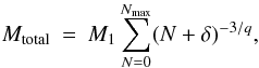 (3)where δ is a random number in the [0, 1] interval and M1 = 4πρ/3C. Since the total mass is fixed, M1 (or C) is determined from the last equation, and individual masses can be found from Eq. (2).
In the context of the discussion about the objects observed in the Kuiper belt and the size of the current irregular satellites, we decided to adopt q = 1.3. Putting the pieces together, we consider the first close encounter between an original planetesimal and Uranus. Our strategy is to substitute the original approaching planetesimal by 500 new masses, that is, m1, m2, ... m500, and for the first two masses we set m1 ~ mPluto and m2 = m1/2. The remaining mass is divided among the other 498 particles according to Eq. (2). We refer to these above resulting masses as “cloned particles”. In the second encounter, the process is repeated, although for the new m1 it is assigned an intermediary value between m1 and m2 values of the previous encounter. Therefore, each original approaching planetesimal is divided into another 500 particles and once the number of Pluto-sized particles reaches 10% of Nenc, the inclusion of Pluto-sized particles (m1 and m2) is stopped so that each massive planetesimal is fully divided into 500 particles according to Eq. (2). The technique of defining two massive masses during the first encounters is irrelevant because afterwards all these encounters will be distributed in a random way. Therefore, to compute the individual effect of each close encounter on the satellites, we attempt to create a local environment that resembles the original disk in the past. Many other criteria could of course, have been applied to set values for the masses. We adopted this distribution after several successful tests and considering that this is an easy way to take into account the existence of some Pluto-sized planetesimals in the past, as pointed in Levison et al. (2008) and Morbidelli et al. (2009b). Moreover, with q = 1.3, the current values of the masses of the irregular satellites can also be easily considered in the model.
Summarizing, the initial planetesimals considered in the previous section that had close encounters with Uranus, give birth to 500 new clones, whose total combined mass is the same as the parent planetesimal (≈1.05 × 10⁻⁸ M⊙). To each clone, we assign an individual mass following two basic ideas: the percentage of the Pluto-sized objects of the original disk is preserved when planetesimals are fragmented into new pieces and the masses of these resulting “cloned particles” follow a power-law distribution. This procedure is repeated for all the original encounters that occurred during a successful run of Nice model. Each “cloned particle” with its mass, position, and velocity is randomly archived in a unique file. The final step is to re-run the original migration model, where the planets are retrieved from the templates compiled in Sect. 4 and some target satellites are attached to Uranus. To compute the effect of these “cloned particles” on the satellites, the code extracts, sequentially, from the above-mentioned file, one intruder at a time inserting it into the Mercury integrator. These planetesimals are injected periodically at some time interval Δt for each original encounter. However, the value of Δt is not the same for the whole integration, since the number of planet-planetesimal encounters is very small at the beginning of the integration and after that, during the passage through the 2S:1J resonance, this number increases drastically. In general, the number of these encounters usually increases during the close encounters between Uranus and Neptune, while in the absence of planetary encounters, the number is small. In other words, Δt is defined during the first simulation when the templates of migration were compiled. Therefore, short or long Δt is adopted according to the number of close encounters that occur during some fixed time interval. This means that some Δt can be shorter than the period of orbit precession of the attached satellites, although this is just a consequence of what really happened in the original migration and we do of course have to preserve this feature in the second integration.
In Fig. 3, we show the number of planet-planetesimal encounters during the time evolution of the planets, i.e., the time variation in the semi-major axes of Uranus and Neptune for each model as given in Fig. 1 is also plotted. The scale on the right vertical axis of each panel shows the number of encounters between the planetesimal and Uranus. As stated before, the majority of the encounters occur during the 2S:1J resonance, when Uranus and Neptune have several close approaches. Although not clearly shown, in model M4-2S:1J, after t = 1.5 × 10⁷ the number of encounters is very small, as in the remaining cases. To confirm this, we extended, as we show in Fig. B.1, the integration to 100 Myr and observed that the number of encounters after the passage through the 2S:1J resonance is almost negligible.
 |
Fig. 3 Full and gray lines: semi-major axes of the planets during migration. Crosses: number of planetesimal-Uranus encounter (right vertical axis). The majority of the encounters occur during the passage through 2S:1J resonance. |
5. Uranus’ satellites
We investigate the behavior of the regular and fictitious satellites of Uranus under the action of migration. We integrate the five inner satellites (M = Miranda, A = Ariel, U = Umbriel, T = Titania, and O = Oberon), as well as six fictitious satellites sk = (s1,s2,s3,s4,s5,s6) placed beyond Oberon whose semi-major axes are 27.5 RU, 33 RU, 39.6 RU, 47.5 RU, 57 RU, and 68.4 RU, respectively. These values were considered in the context of the empirical relation ai + 1 ≈ 1.2ai, where a0 is the semi-major axis of Oberon, a1 is the semi-major axis of s1, and so on. The remaining initial conditions (eccentricity and inclination) are given in Table 2. For the regular satellites, we take the current values, apart from changing Miranda’s inclination to zero (see Table 2).
For the mass of the regular satellites, we considered the following values in terms of M⊙mM = 3.31 × 10⁻¹¹ (D ≈ 471.45 km), mA = 6.80 × 10⁻¹⁰ (D ≈ 1156.51 km), mU = 5.89 × 10⁻¹⁰ (D ≈ 1169.18 km), mT = 1.77 × 10⁻⁹ (D ≈ 1578.38 km), and mO = 1.52 × 10⁻⁹ (D ≈ 1524.42 km). The diameters were estimated by adopting a density (g/cm3) ρM = 1.20, ρA = 1.67, ρU = 1.40, ρT = 1.71, and ρO = 1.63.
For the fictitious satellites, we have ms1 = 1 × 10⁻¹⁰ (D ≈ 724.25 km), ms2 = 1 × 10-11 (D ≈ 336.17 km), ms3 = 1 × 10-12 (D ≈ 156.03 km), ms4 = 6 × 10-13 (D ≈ 131.60 km), ms5 = 3 × 10-13 (D ≈ 104.45 km), and ms6 = 1 × 10-13 (D ≈ 72.42 km), and the density was fixed to 1 g/cm3 for all of them.
5.1. Encounters without planetesimals
To study the dynamics of the regular and si satellites, first of all, we consider only the effect of the planetary encounters. In the Mercury package, the hybrid option integrator was selected with a time step fixed to 1/20 of Miranda’s orbital period. The disturbers are the neighbouring planets, the Sun, and J2, as well as mutual perturbations among all the satellites. The motion of the planets is given in terms of the interpolating polynomials obtained according to the technique described in Sect. 4. The integrations are limited to only 5 or 10 Myr, since after that, additional planetary close encounters if exist, are very rare. Similar investigations of the satellites of Uranus in this scenario were presented by us in some previous works, where Jupiter and Saturn were however fixed at the 2S:1J resonance, so that the variations were much more pronounced (Yokoyama et al. 2008) and in many cases the escape of the regular satellites were observed.
In Table 2, all the regular satellites survive retaining their small eccentricities and inclinations. The fictitious satellites s1, s2, s3, and sometimes s4, usually survive with rather low values of eccentricity, while the remaining s5 and s6, in general experience collisions, or are ejected and in this case, the name of the corresponding object that participated in the collision is indicated in the place of the final elements (see details in Table 2). We note that these si have highly disturbed orbits because they may collide with distant and interior regular satellites. For instance, s5, which started with semi-major axis 57 RU, collided with Miranda (model M5). In addition, s6 collided with Ariel (model M1).
Results of 5 and 10 Myr integration time, considering the main regular satellites of Uranus and 6 fictitious satellites beyond Oberon (placed on LLP).
We also, note that the initial inclinations of the satellites were considered on the local Laplace “plane” (LLP) since in the case of distant si satellites, if they existed in the past they probably originated close to this plane. The local Laplace “plane” is a convenient surface whose orientation varies according to the distance between the planet and the satellite. If a satellite is placed on this “plane”, eventual large periodic perturbations owing to the Sun on the satellite, can be cancelled by the oblateness perturbations, so that the orbital plane of the satellite referred to LLP precess uniformly. Roughly speaking, for very short distances, this plane coincides with the equator, while for large distances it coincides with the planet-sun orbital plane (Sinclair 1972). The relationship between LLP and equator plane is given by the equation 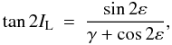 where
where 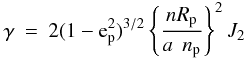 and IL is the inclination of the LLP with respect to the Uranus’ equator, ε refers to the obliquity of the planet, n is the mean motion of the satellite whose semi-major axis is a, Rp is the equatorial radius of the planet, and np is the mean motion of the Sun. With the above relation, we can place any satellite on the LLP.
A simple calculation shows that γ is the ratio of the oblateness and solar perturbation. Moreover, for γ = 1 we obtain ac as defined in Eq. (1). Therefore, the Laplacian plane is close or far from the equator depending on γ.
We note that in the absence of planetesimals, all the regular satellites always remain quite immune to the planetary close encounters of migration. We can see that placing si satellites on LLP, the effect of the Lidov-Kozai resonance decreases, although this was not enough to avoid the destabilization of s5 and s6. Some close encounters either between Uranus and Neptune, or between Uranus and Saturn, that excite si seems to have a stronger effect. In Table 2, the initial inclination of si are indicated by a fraction (I1/I2). The first number of the fraction (I1) refers to the initial inclination of si when Uranus starts its migration at aU = 11.5 AU (M1, M2, M4, or M5) and I2 when Uranus starts at aU = 14.2 AU (M3). These Ik values indicate the inclination of the satellite (on LLP) with respect to the Uranus’ equator.
5.2. Inclusion of the planetesimals
We now include the effect of the planetesimals. We again integrate the si fictitious satellites together the five regular satellites (Miranda, Ariel, Umbriel, Titania, and Oberon). Periodically, we inject the “cloned particles” according to each close encounter involving the “selected” planetesimals as described in Sect. 4. In Sect. 3, we selected five migrational models. Each model is integrated considering four different random insertions of the planetesimals.
This time, during migration, the satellites suffer different situations of close approach owing to the presence of the planetesimals. In most cases, we adhere to the original version of the Mercury package, which assumes an inelastic collision, that is, based on the conservation of the linear momentum, the MERGE subroutine adds mi and mj (masses of the target and projectile, respectively) to form a single mass mk. This merging of masses is the simplest way to treat collisions, and usually when mi and mj are of different order, the technique works quite well. However, in some situations, there are other aspects of the problem. For example, in the region populated by the si satellites we consider a collision involving a satellite and a planetesimal with masses mi and mj, respectively. If both are on the same order and a new body is created, its mass will be about twice the value of mi (or more). Under these conditions, our calculations show that, in general, the abrupt “birth” of a massive body (mk), close to or inside the system of si satellites, causes a clear instability: a given si satellite can become strongly disturbed and invade the region of regular satellites. Eventually even mk might do the same. Significant perturbations take place and new collisions can appear, particularly when mk remains (even temporally) as a satellite of the planet. If collisions in cascade occur, a significant part of the whole system can be destabilized.
The problem of impacts has been studied by several authors, mainly in asteroidal and recently in irregular satellite problem (Bottke et al. 2010). A general treatment of the events during a collision between a target body and a projectile, usually involves three situations: cratering, shattering, and dispersing (Benz & Asphaug 1999).
To better characterize these impacts, authors define a specific energy Q (kinetic energy of the projectile per unit of the mass of the target). In this way, we define  to be the critical impact energy. This is the energy needed to disrupt the target and send about 50% of its mass away. For
  , we have a cratering event, a
  catastrophic event, and a
  super-catastrophic event where in some cases, both objects are pulverized (Bottke et al. 2010). The values of
  for different materials are determined from sophisticated techniques and laboratory experiments, usually for ice and basalt, when considering limited impact velocities in the range 2.5–7.5 km s-1 (Durda et al. 2004; Benz & Asphaug 1999; Bottke et al. 2010, etc.). In all these experiments, the results also depend on the impact angles and the size of the targets. According to Bottke et al. (2010), in some situations when the smashing bodies have masses of the same order, in the super-catastrophic cases (when ), the pulverizing of both objects takes place. Adopting some similar data (-curve) given in Bottke et al. (2010), we confirmed the existence of some highly super-catastrophic collisions () when mi ≈ mj in our problem. In addition, in Uranus’ case, the regular satellites are very close to the planet, therefore some high impact velocities reaching 13.5 km s-1 can appear. On the other hand, the impact angles reach almost all values in the [0°,180°] interval. Finally, the bulk density of the major satellites of Uranus is in the interval [1.2 g/cm3, 1.7 g/cm3] and the global ratio ice/rock is close to 1. As we can see, for asteroids or irregular satellites (objects far from the planets), the approximate values of the basic parameters (, the angle of impact, velocities, material involved, size, etc.) are known. However, in the case of regular satellites (especially for Uranus’ satellites) the space of parameters seems to be much larger and somewhat more complex. Moreover, some collisions can generate fragments that can either escape or re-accumulate, usually around some large fragment. In this sense, a re-accumulation may produce a new regular satellite replacing those that were destroyed in the collision. For a rigorous treatment of the dynamics of the close approach involving satellites, it would be necessary to consider all these details, and of course appropriate values for the involved materials.
Therefore, in our problem, owing to the lack of additional information, we decided to consider only a first order approximation of the problem: whenever mi and mj are of different orders, we adopt the original inelastic version of mass conservation in the Mercury package. On the other hand, when the masses are on the same order, we considered a super-catastrophic event (Bottke et al. 2010). We then, add the two pulverized masses to the planet such that we maintain the conservation of the momentum.
The study of a possible re-accumulation of the fragments into a single body is probably dissimilar to the classical cases because the pieces to be accreted are submitted to a non-negligible perturbation of other massive and close satellites. In this way, even in the case of partial pulverization, a possible re-accumulation of the ejected material, originating in a new object, will not be considered in this work.
Then, considering these ideas, and placing si satellites on the LLP, we obtained Tables 3 and B.1. The first table we call “successful runs” and in the last table we have the cases when at least one regular satellite is lost, usually due to a collision, either with another satellite or with a massive planetesimal. We classify these cases as “unsuccessful runs”. Table 3 presents the main results. It shows the outcome of the final orbital elements of the regular satellites. In this table, all the regular satellites survived (12 runs). In the remaining eight unsuccessful runs (Table B.1), a significant number of the regular and si satellites are destabilized. As expected, usually s5 and s6 are the weakest in terms of stability. In general, the eccentricities and inclinations of the regular satellites remained small, although some exceptions are very clear. For instance, Miranda, the smallest satellite, has final values of e ≈ 0.294, I ≈ 14.26°, (M1, Job4) and e ≈ 0.118, I ≈ 2.38° (M2, Job2).
Comparing Table 3 with the previous tables, the effect of the planetesimals becomes very clear. Without their presence, all the regular satellites remain quite stable, so that the cause of the instabilities in the regular satellites is essentially the action of the planetesimals. Practically, they are able to destabilize the fictitious satellites not only those placed beyond ac, but also satellites with a > aOberon. The destabilization of si satellites occur mostly because of either collisions between themselves or with the regular satellites. On the other hand, regular satellites can be strongly affected whenever an intruder of mass either greater than or on the order of 3.31 × 10⁻¹¹ M⊙ (Miranda’s mass), approaches sufficiently close to that of Uranus (about ≈ 10 RU). This was first pointed out in Beaugé et al. (2002), although the authors used planetesimals with much higher masses.
As we see, satellite-planetesimal close encounters are very frequent and significantly influence the final architecture of the satellite system. Therefore, not only an inelastic collision but some additional scenarios as described in Benz & Asphaug (1999), Durda et al. (2004), and Bottke et al. (2010) would be necessary.
Although not shown, for completeness, we repeated all these simulations (13 successful runs), placing all the satellites (including si) on the equator. The final results are very similar. We conclude that in our 25 successful simulations, thanks to the effect of the planetesimals, the fictitious satellites beyond Oberon are usually destabilized.
The presence of some massive planetesimals (Pluto-sized) in our disk, is a quite reasonable hypothesis considering that they actually exist in the exterior Kuiper disk. Moreover, as pointed out in Nesvorný et al. (2007) there is no reason to believe that the only massive objects to have been accreted into the disk were the four giant planets.
It is well-known that under certain conditions, such as the initial semi-major axis and rotational state of the planet (for a review, see Ferraz-Mello et al. 2008) the tidal effect is able to either decrease or increase some orbital elements of the satellites. In this work, for the initial semi-major axis of the regular satellites we adopted the current values. Perhaps, for smaller values, closer to Uranus, they could more successfully resist the encounters with massive planetesimals, and after that, owing to tidal effects their eccentricities and inclinations could be damped to their current values, and the semi-major axes could increase to their present values. Another possible source of damping is the satellite dynamical friction. Collisions would probably, provide additional material to form a local disk around the planet. This disk might be able to cause efficient dynamical friction on the satellites. Some preliminary studies of dynamical friction indeed indicate damping inclination and eccentricity might depend on the local disk around the planet. Therefore, some excited values of the eccentricity and inclination from Table 3 could be damped via the above mechanisms.
We finally consider Fig. B.1 (Appendix B). In a similar way to Fig. 3, this figure shows the number (N) of Uranus-planetesimal close encounters, but this time for a 100 Myr migrational time. This is usually the time required for a typical migration in order to get the four planets to their current eccentricity, inclination, and semi-major axis. We note, however, that the majority of the close approaches with Uranus occur when Jupiter and Saturn are in 2S:1J resonance. Usually, after 5 or 10 Myr this number is very small and in principle, we believe that it is unlikely that drastic change can occur for the remaining satellites after that. In addition to the cpu-time, this is another reason why we considered only 5 or 10 Myr in the integrations of this section.
Finally, we note that in Nesvorný et al. (2007) the authors considered massless planetesimals and the set of regular satellites were neglected. In our case, all the planetesimals that participate in the close encounters have a specific mass. These massive planetesimals interact with all satellites (regular and si fictitious satellites). In particular, massive planetesimals are responsible for cleaning the si objects placed beyond Oberon. On the other hand, the inclusion of the regular satellites becomes important in the capture of planetesimals as we now show (see Sect. 6).
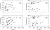 |
Fig. 4 a), b) Captured objects (full circles) in the case (M2, Job4) for planetesimals injected from ≈ 100 RU. c), d) same as a), b) but now all planetesimals were injected from ≈ 300 RU. Inclination on panels b) and d) refers to the Uranus’ orbital plane. Triangles refer to current irregular satellites. |
5.3. The si satellites
In Sect. 2, we discussed both ac and the possible absence of si satellites beyond Oberon. An additional interesting problem is the current obliquity of Uranus.
Mosqueira & Estrada (2003) and Estrada & Mosqueira (2006), in their model of satellite formation, note that regular satellites of Uranus can be formed within a disk of radius ≈ 57 RU. We note that this value is in quite close agreement with the distances predicted based on our value of ac as we note in Sect. 2.
On the basis of this result, Boué & Laskar (2010) considered a satellite (sBL) placed at 50 RU to construct a collisioness scenario for the Uranus’ obliquity. These authors considered a rather high mass for their satellite but one decisive key for the success in reproducing the tilt of Uranus is the presence of a sBL satellite in the evolutionary dynamics of Uranus’ obliquity.
In view of these studies, particularly Mosqueira & Estrada (2003) and Estrada & Mosqueira (2006), it is therefore quite reasonable to take into account the existence of some si satellites as we did, and to see their evolution during the planetary migration.
The second decisive result of Boué & Laskar (2010) is that their satellite must be destabilized after some time, and this is exactly what we have found in this work. In our case, in almost all cases, si with a ≥ 27.5 RU can be destabilized in the presence of the planetesimals, while almost all si with a ≥ 47.5 RU are ejected by planetary close encounters, without planetesimals.
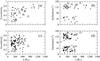 |
Fig. 5 a), b) Thirty-four captured objects (full circles) in the case (M2, Job4) for planetesimals injected from ≈ 200 RU; c), d) same as a), b) but for M2, Job3 (94 captures). Inclination on panels b) and d) refers to the Uranus’ orbital plane. The original parent planetesimal was cloned to 1000 new objects. Triangles refer to current irregular satellites. |
6. Capture of irregular satellites
When injecting planetesimals that approach Uranus, a natural consequence of this process is the capture of some planetesimals by the planet. In the previous sections, most of the integrations are limited to 5 or 10 Myr. Even so, it is very instructive to examine the planetesimals that become captured during the experiments shown in Sect. 5. Figure 4a,b shows  and
and  for (M2, Job 4). It shows the mean elements of the captured planetesimals after 5 Myr.
To develop an ultimate scenario of the planets and their captured satellites, we should integrate the whole system up to 100 Myr. This would be a very time-consuming simulation, mostly because of the short period of the regular satellites and also the number of captured satellites.
In principle, after 5 or 10 Myr, almost no more planetary close encounter should occur. After this time, some additional experiments have also shown that the number of important planet-planetesimals encounters not only decreases rapidly as well as the net effect of them seems to be insignificant (see Fig. B.1). Therefore, it is reasonable to believe that the capture of planetesimals shown in our simulations, is a mechanism that can generate a collection of objects around Uranus, which can lead to the current irregular satellites of the planet. After several experiments, we concluded that different models Mi have different efficiency capture. Usually, the statistics of the captured objects can be increased in different ways: in Sect. 4.1 instead of cloning one original object to 500, we can do it for a larger number. Another strategy is to consider planet-planetesimal encounters with distances greater than 100 RU. Finally, the number of close encounters we detected was obtained by checking the distance planet-planetesimal every 14 years. If this time interval had been decreased, more encounters would certainly have been collected.
Figure 4c,d is similar to Fig. 4a,b but this time, instead of 100 RU, all planet-planetesimals encounters within 300 RU were collected. For this reason, the number of captures is larger than in the previous case. In general, the agreement of our results with the properties of real satellites is good, in spite of the limited number of captures in the present model.
In all these figures, none of the  is smaller than ≈ 100 RU. This lower limit is in good agreement with the results for current satellites. Our experiments also indicate that the current regular satellites in the simulations determine this lower limit.
In the process of capture, the size of time step of the integrator (Δh) is important, that is, a short Δh increases the probability of captures. Usually, in the presence of the regular satellites, Δh remains small because the period of the inner satellite is short.
Figure 5a,b and c,d are similar to those shown previously, but this time, all the planet-planetesimals encounters within 200 RU were considered, and the original parent planetesimal was cloned to 1000 new objects. We note that the capture efficiency is significantly higher and the improvement is very clear when compared to real satellites. It is also remarkable that the captured objects coherently maintain a minimum distance of  . These two last figures depict a very straightforward scenario of the capture of irregular satellites.
As pointed in Nesvorný et al. (2007), the number of the retrograde captures in all figures, is almost similar to those of the prograde captures. This relation contradicts the current distribution seen today. However, a final scenario of the relation between these two populations probably requires more investigation, especially of the collisional evolution (Bottke et al. 2010). First of all, the number of captured objects should increase. We can improve the statistics of captured objects exploiting the above-mentioned strategies. Evolving the whole group of objects for longer times and considering their mutual interactions seems to be necessary to compute future collisions among them. Since in our model all the captured satellites have a mass, a simulation computing the collisions among them could be important to forming the long-term scenario. Before some stabilization of this system, it may be early to define the ratio of prograde-retrograde objects.
Since the semi-major axis is at least 100 RU, the dominant disturber is the Sun. In this case, the Lidov-Kozai resonance usually takes place whenever the inclination (I), referred to the orbital plane of the disturber is ≈ 39° ≤ I ≤ ≈ 141° (Yokoyama et al. 2003). If I is inside this interval, the eccentricity usually undergoes large variations that can cause the ejection of the satellite. This is why in the figures of this section there is a clear gap in the vicinity of I = 90°. However, if the argument of the pericenter ω were captured in a deep libration, the amplitude of the variation of the eccentricity might be not so drastic and the satellite might survive (for at least some time, Fig. 5c,d).
Simple simulations show that planar satellites (with respect to the equator) beyond Oberon usually cannot survive. More precisely, the combination of distant satellites and high obliquity of the host planet, enhances the perturbation of the Sun, so that a large variation in the eccentricity is unavoidable.
7. Conclusion
We have made an exploratory analysis of the effect of the planetary migration, basically on the regular satellites. Following Nice model, we have concluded that Oberon is indeed the last regular satellite of Uranus, which resists the close encounters during migration. All other satellites with semi-major axis above 22.8 RU, if they existed, were probably destabilized. The distant satellite (a = 50 RU) considered by Boué & Laskar (2010) is an example of one that is easily destabilized. As Uranus’ ε is high, destabilization is more common for equatorial satellites formed beyond Oberon. Distant satellites placed on the LLP are also destabilized, mostly due to planetary close encounters and also collisions among themselves. We have also concluded that the existence of a large number of planetesimals with masses above ≈ 10-9 M⊙ in the disk becomes problematic if they penetrate the region of the regular satellites. The excitation that they cause in the orbits of the regular satellites (mainly in the inclination) is significant and sometimes incompatible with the current values. Some efficient mechanism, e.g., tidal effect, or satellite dynamical friction probably would have enabled us to dampen these parameters to the current values.
Owing to the high sensitivity of the dynamical system in migration, we developed an interpolating technique: a database of the orbits of planets on a successful migration is previously recorded and after that only the satellites are integrated under the action of the planets whose orbits can be retrieved from the database. With these techniques, we computed the effect of the close encounters involving planets and planetesimals. These encounters allowed us to study the capture of objects that are candidates to be the current irregular satellites. The technique works quite well and we already have some results for Jupiter’s satellites, even considering that this planet does not experience significant numbers of planetary close encounters during migration. The efficiency of the captures clearly depends on the time step of the integrator, while the stability of the regular satellite and also the si satellites, strongly depends on the masses of the involved planetesimals.
Since captured satellites may acquire an initially large inclination, we examined the dynamics of these objects: owing to Lidov-Kozai resonance they can be easily destabilized because their eccentricities then increase to very large values. We also showed the importance of the effects of the Sun and of the oblateness for just-captured objets (see Appendix A).
Online material
Appendix B: Complementary tables and figures
Figure B.1 is similar to Fig. 3, but now extended to 100 Myr. We note that the general behaviour of the elements after 5 or 10 Myr is almost unchanged.
Table B.1 refers to the non-successful case, that is, at least one of the current regular satellite is lost during migration. In the table of this Appendix, when a given satellite experiences a collision with another satellite, in the column of the given satellite we indicate this with M, A, U, T, O, and si (the name of the participant of the collision). On the other hand, if the participant is a planetesimal, we indicate it with m/d, where m is the mass ( × 10-9 M⊙) and d is the diameter (in km) of the planetesimal.
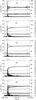 |
Fig. B.1 Similar to Fig. 3 but time extended to 100 Myr. Here we also show the evolution of the perihelion (q) and aphelion (Q) of the planets during migration. |
Acknowledgments
We thank Rodney S. Gomes for allowing us to use his code and also for very fruitful discussions. An anonymous referee is gratefully thanked for very important suggestions. We also thank Professor R. M. Lagos for helping us with the English language. This work was supported by FAPESP and CNPQ. T. Yokoyama dedicates this work to the memory of Elizabeth M. L. Maegawa Yokoyama.
References
- Agnor, C. B., & Hamilton, D. P. 2006, Nature, 441, 192 [NASA ADS] [CrossRef] [PubMed] [Google Scholar]
- Beaugé, C., Roig, F., & Nesvorný, D. 2002, Icarus, 158, 483 [CrossRef] [Google Scholar]
- Benz, W., & Asphaug, E. 1999, Icarus, 142, 5 [NASA ADS] [CrossRef] [Google Scholar]
- Boué, G., & Laskar, J. 2010, ApJ, 712, L44 [NASA ADS] [CrossRef] [Google Scholar]
- Bottke, W. F., Nesvorný, D., Vokhrouhlický, D., & Morbidelli, A. 2010, ApJ, 139, 994 [Google Scholar]
- Brasser, R., Morbidelli, A., Gomes, R., Tsiganis, K., & Levison, F. H. 2009, A&A, 134, 1790 [Google Scholar]
- Burns, J. A. 1986, in Satellites, ed. J. A. Burns, & M. S. Matthews (Tucson: Universty of Arizona) [Google Scholar]
- Callegari, Jr N., & Yokoyama, T. 2008, Cel. Mech. Dyn. Astron., 102, 273 [NASA ADS] [CrossRef] [Google Scholar]
- Canup, R. M., & Ward, W. 2000, BAAS, 32, 1105 [NASA ADS] [Google Scholar]
- Canup, R. M., & Ward, W. 2006, Nature, 441, 834 [NASA ADS] [CrossRef] [Google Scholar]
- Chambers, J. E. 1999, MNRAS, 304, 793 [NASA ADS] [CrossRef] [MathSciNet] [Google Scholar]
- Ćuk, M., & Gladman, B. J. 2005, ApJ, 626, L113 [NASA ADS] [CrossRef] [Google Scholar]
- Durda, D., Bottke, W. F., Enke, B. L., et al. 2004, Icarus, 167, 382 [NASA ADS] [CrossRef] [Google Scholar]
- Estrada, P. R., & Mosqueira, I. 2006, Icarus, 181, 486 [NASA ADS] [CrossRef] [Google Scholar]
- Fernandez, J. A., & Ip, W. H. 1996, Planet. Space Sci., 44, 431 [NASA ADS] [CrossRef] [Google Scholar]
- Ferraz-Mello, S., Rodriguez, A. C., & Hussmann, H. 2008, Cel. Mech. Dyn. Astron., 101, 171 [NASA ADS] [CrossRef] [Google Scholar]
- Goldreich, P. 1966, History of the Lunar Orbit Reviews of Geophysics, 4, 411 [Google Scholar]
- Goldreich, P., Murray, N., Lonagaretti, P. Y., & Banfield, D. 1989, Science, 245, 500 [NASA ADS] [CrossRef] [PubMed] [Google Scholar]
- Gomes, R. S., Tsiganis, K., Morbidelli, & Levinson, H. F. 2005, Nature, 435, 466 [NASA ADS] [CrossRef] [PubMed] [Google Scholar]
- Hahn, J. M., & Malhotra, R. 1999, ApJ, 117, 3041 [Google Scholar]
- Jewitt, D., & Haghighipour, N. 2007, ARA&A, 45, 261 [NASA ADS] [CrossRef] [Google Scholar]
- Lanczos, C. 1970, The variational principles of mechanics, fourth edition (University of Toronto Press) [Google Scholar]
- Levison, H. F., Morbidelli, A., Vanlaerhoven, C., Gomes, R., & Tsiganis, K. 2008, Icarus, 196, 258 [NASA ADS] [CrossRef] [Google Scholar]
- Malhotra, R. 1993, Nature, 365, 819 [CrossRef] [Google Scholar]
- Morbidelli, A. 2010 [arXiv:1010.6221v1] [Google Scholar]
- Morbidelli, A., Levison, H. F., Tsiganis, K., & Gomes, R. 2005, Nature, 435, 462 [NASA ADS] [CrossRef] [PubMed] [Google Scholar]
- Morbidelli, A., Tsiganis, K., Crida, A., Levison, F. H., & Gomes, R. 2007, ApJ, 134, 1790 [Google Scholar]
- Morbidelli, A., Brasser, R., Tsiganis, K., Gomes, R., & Levison, F. H. 2009a, A&A, 134, 1790 [Google Scholar]
- Morbidelli, A., Levison, H. F., Bottke, W., Dones, L., & Nesvorný, D. 2009b, Icarus, 202, 310 [NASA ADS] [CrossRef] [Google Scholar]
- Mosqueira, I., & Estrada, P. R. 2003, Icarus, 163, 198 [NASA ADS] [CrossRef] [Google Scholar]
- Nesvorný, D., Vokrouhlický, D., & Morbidelii, A. 2007, A&J, 133, 133 [Google Scholar]
- Nogueira, E. C. 2008, Doctor Thesis, Universidade Federal do Rio de Janeiro, Brasil [Google Scholar]
- Sinclair, A. T. 1972, MNRAS, 155, 249 [NASA ADS] [Google Scholar]
- Stuchi, T. J., Yokoyama, T., Corrêa, A. A., et al. 2008, Adv. Space Res., 42, 1715 [NASA ADS] [CrossRef] [Google Scholar]
- Trujillo, C. A., Luu, X. J., Bosh, A. S., & Elliot, J. L. 2001, AJ, 122, 2740 [NASA ADS] [CrossRef] [Google Scholar]
- Tsiganis, K., Gomes, R., Morbidelli, A., & Levinson, H. F. 2005, Nature, 435, 459 [NASA ADS] [CrossRef] [PubMed] [Google Scholar]
- Yokoyama, T. 2002, Planet. Space Sci., 50, 63 [Google Scholar]
- Yokoyama, T., Santos, M. T., Cardin, G., & Winter, O. C. 2003, A&A, 401, 763 [NASA ADS] [CrossRef] [EDP Sciences] [Google Scholar]
- Yokoyama, T., Deienno, R., & Nogueira, E. C. 2008, Perturbations on regular satellites as consequences of the planetary migration, 40th DPS Meeting, Program Update, Ithaca, New York, USA [Google Scholar]
- Yokoyama, T., Deienno, R., Nogueira, E. C., et al. 2009, The role of the Uranus’ obliquity on its satellites during the planetary migration, IAU XXVII General Assembly, Abstract book, 64, Rio de Janeiro, Brasil [Google Scholar]
Appendix A: The role of the oblateness and the obliquity of the planet
Here we show the importance of the oblateness of the central body when either the high inclination or high obliquity of the planet is involved. During migration and depending on the close encounters, a captured planetesimal may become a permanent satellite of the planet. For Uranus, owing to its high obliquity, the combined effect of the oblateness and satellite-planet distance may play an important role.
Taking a simplified model, the secular dynamics of a single particle can be studied considering only the main disturbers: Sun and the oblateness. The case of Uranus’ satellites is quite peculiar because the inclination of the orbital plane of the Sun with respect to the equator (obliquity) is very large (ε ≈ 97.8°).
We now consider the equator and the orbital plane of the planet. Some simple geometrical relations involving these two planes are:  (A.1)where
  In these relations, the argument of the pericenter, longitude of the node, and inclination of the satellite referred to the equator are denoted by ω, Ω, and I, respectively. Index “a” is added when referred to the orbital plane of the planet, whose obliquity is ε.
We note that relations connecting the two reference planes (equator and orbital plane) define a canonical transformation (w,Ω,G,H) → (wa,Ωa,Ga,Ha) as can be easily checked by calculating the classical Lagrange’s brackets using Eq. (A.1) (Lanczos 1970). As (w,Ω,G,H) are the well-known Delaunay canonical variables, from the first line in Eq. (A.1) we have  where k2 is the classical gravitation constant and Mp is the mass of the planet.
In a equatorial reference system fixed in the center of the planet, the disturbing function owing to the oblateness on a satellite is  (A.2)and for the solar perturbation
  (A.3)In either Eqs. (A.2) or (A.3), terms of order three in the ratio Rp/r or r/r⊙ were neglected.
The meaning of the coefficients are
-
M⊙: mass of the Sun;
m: mass of the satellite;
r,r⊙: position vector of the satellite and of the Sun;
φ,S: latitude of the satellite and Sun-satellite angular distance;
J2: oblateness coefficient.
 (A.4)Analogously, taking simple geometric relations, RJ2 with respect to the orbital plane of the planet is obtained
  (A.5)Analogously, with respect to the orbital plane, the average of the solar perturbation is
  (A.6)Additional effects, including close encounters (mostly involving planetesimals) are of course still possible, but all these situations depend on the disk-model and other parameters considered in the migration. Therefore, any primordial satellite or planetesimal that becomes captured, even temporarily, will be disturbed by RJ2 and R⊙ and the magnitude of the perturbations will depend on the distance to both the planet and the Sun. We recall that at the beginning of migration, Uranus’s semi major-axis is about ≈ 11 − 13 AU ending at ≈ 19 AU.
In terms of the classical Delaunay variables, the secular motion of the satellite is given by the Hamiltonian H = RJ2 + R⊙. Now, if RJ2 is the predominant term of the Hamiltonian such that R⊙ is negligible, we can easily conclude that the initially circular and planar orbits keep these parameters almost unchanged, since no angular coordinate occurs in Eq. (A.4). On the other hand, when R⊙ is the dominant part, we usually neglect RJ2. In this case, from Eq. (A.6) we conclude that Ha is a constant because Ωa is a kinosthenic variable. From the definitions of Ha and Ga and from Eq. (A.1), we have that  (A.7)where L = (k2Mpa)1/2.
As before, we assume an initial circular and planar orbit with respect to the equator. This means that e = ea ≈ 0 and Ia ≈ ε. Therefore, the constant Ha is fixed to Ha ≈ Lcosε and from the above equation  (A.8)If we consider the case of Uranus where ε ≈ 90°
 and since Ω circulates we see that both eccentricity and inclination (with respect to the equator) can undergo large variation. If Uranus’ oblateness is neglected, then a simple numerical integration shows that for semi-major axis aU = 12 AU, a planar primordial satellite with a = 10 RU escapes in 110 thousand years. On the other, hand a if current J2 is assumed, then even a satellite with a = 22.8 RU (Oberon) remains quite stable. The instability for the first case is the classical Lidov-Kozai resonance. Therefore, the combined effect of RJ2 and R⊙ is important so that in some situations when the planet is close to the Sun, they cannot be neglected. We can say that the oblateness enhances the stability of the satellite (Yokoyama et al. 2008; Stuchi et al. 2008).
In the case of Jupiter, we have ε ≈ 0, so that Ia ≈ I and from Eq. (A.8), we have that  (A.9)We note that for ε ≈ 0 the above relation is valid for any J2. Therefore since I ≈ Ia, then for an initial value of Ia ≈ 0 the eccentricity and inclination must remain small all the time according to Eq. (A.9). However, for large initial inclination (Ia ≈ 90°) we have that 0 ≈ (1 − e2)1/2cosI, hence eccentricity and inclination can undergo significant variation provided that R⊙ is not negligibly small (the satellite cannot be so close to the planet, otherwise RJ2 dominates and both inclination and eccentricity would remain almost unchanged).
In Table 2 of Sect. 5, the s5 and s6 satellites are destabilized in all runs. Owing to its large distance from Uranus, this is a typical case of the instability caused by the Lidov-Kozai resonance. The eccentricity attains high values very rapidly and therefore any additional perturbation (e.g. future close encounter) can destabilize the satellite. However, some numerical experiments indicate that while an isolated object is rapidly destabilized if placed near ac, when we consider a group of more satellites interacting themselves, the individual escape seems to be
uncertain, or much more time is needed for it to occur. This may be why some si persists with a relatively small eccentricity and inclination in Table 3. Very close to ac, there is a balance between the oblateness and solar perturbations such that the Hamiltonian H = RJ2 + R⊙ is not a single degree of freedom problem and the secular dynamics might be more complex.
All Tables
Results of 5 and 10 Myr integration time, considering the main regular satellites of Uranus and 6 fictitious satellites beyond Oberon (placed on LLP).
All Figures
|
Fig. 1 Models Mi: time evolution of the semi-major axes of the planets during the passage through 2S:1J resonance. |
| In the text | |
|
Fig. 2 Top: three satellites of Uranus (a = 25 RU, a = 40 RU, a = 55 RU) are included in a previous simulation. Bottom: same as on the top, including only two satellites: (a = 30 RU, a = 60 RU). The path of the ice planets changes completely with the inclusion of these satellites. |
| In the text | |
|
Fig. 3 Full and gray lines: semi-major axes of the planets during migration. Crosses: number of planetesimal-Uranus encounter (right vertical axis). The majority of the encounters occur during the passage through 2S:1J resonance. |
| In the text | |
|
Fig. 4 a), b) Captured objects (full circles) in the case (M2, Job4) for planetesimals injected from ≈ 100 RU. c), d) same as a), b) but now all planetesimals were injected from ≈ 300 RU. Inclination on panels b) and d) refers to the Uranus’ orbital plane. Triangles refer to current irregular satellites. |
| In the text | |
|
Fig. 5 a), b) Thirty-four captured objects (full circles) in the case (M2, Job4) for planetesimals injected from ≈ 200 RU; c), d) same as a), b) but for M2, Job3 (94 captures). Inclination on panels b) and d) refers to the Uranus’ orbital plane. The original parent planetesimal was cloned to 1000 new objects. Triangles refer to current irregular satellites. |
| In the text | |
|
Fig. B.1 Similar to Fig. 3 but time extended to 100 Myr. Here we also show the evolution of the perihelion (q) and aphelion (Q) of the planets during migration. |
| In the text | |
Current usage metrics show cumulative count of Article Views (full-text article views including HTML views, PDF and ePub downloads, according to the available data) and Abstracts Views on Vision4Press platform.
Data correspond to usage on the plateform after 2015. The current usage metrics is available 48-96 hours after online publication and is updated daily on week days.
Initial download of the metrics may take a while.