| Issue |
A&A
Volume 695, March 2025
|
|
|---|---|---|
| Article Number | A276 | |
| Number of page(s) | 13 | |
| Section | Planets, planetary systems, and small bodies | |
| DOI | https://doi.org/10.1051/0004-6361/202453433 | |
| Published online | 27 March 2025 | |
The current impact rate on the regular satellites of Jupiter, Saturn, and Uranus
1
Konkoly Observatory, HUN-REN CSFK, MTA Centre of Excellence ;
Konkoly Thege Miklos St. 15-17,
1121
Budapest, Hungary
2
Centre for Planetary Habitability (PHAB), Department of Geosciences, University of Oslo ;
Sem Saelands Vei 2A,
0371
Oslo,
Norway
3
Earth Life Science Institute, Tokyo Institute of Technology,
Meguro-ku, Tokyo
152-8550, Japan
4
Observatoire de l’Université de Genève,
Chemin Pegasi 51,
1290
Versoix, Switzerland
★ Corresponding author; This email address is being protected from spambots. You need JavaScript enabled to view it.
Received:
13
December
2024
Accepted:
4
March
2025
Abstract
Context. The impact and cratering rates onto the regular satellites of the giant planets are subject to great uncertainties.
Aims. We aim to compute the impact rates for objects with a diameter Di > 1 km onto the regular satellites of Jupiter, Saturn, and Uranus using dynamical simulations of the evolution of the outer Solar System coupled with the best estimates of the current population of objects beyond Neptune, and their size-frequency distribution.
Methods. We analyse the last 3.5 billion years of evolution of the outer Solar System from our database of simulations and combine this with observational constraints of the population beyond Neptune to compute the flux of objects entering the Centaur region. The initial conditions of these simulations resemble the current population. We obtain an improved estimate of the impact probability of a Centaur with the satellites from enacting simulations of planetesimals flying past the satellites on hyperbolic orbits, which agree with literature precedents.
Results. Our impact rate of objects Di > 1 km with Jupiter is 0.001 yr−1, which is 3–6 times lower than previous estimates. Both our impact probabilities with the satellites scaled to the giant planets and leakage rate of objects from beyond Neptune into the Centaur region are consistent with earlier literature estimates. However, our absolute impact probabilities with the giant planets are lower. We attribute this difference to whether the impact probabilities are computed over the whole age of the Solar System including planet migration, or over a shorter interval closer to the present.
Conclusions. Our lower impact rate compared to earlier literature estimates is due to basing our results on the flux of objects coming in from beyond Neptune rather than relying on the current observed impact rate with Jupiter. We stress the importance of clearly stating all parameters and assumptions in future studies to enable meaningful comparisons.
Key words: Kuiper belt: general / planets and satellites: dynamical evolution and stability / planets and satellites: gaseous planets
© The Authors 2025
 Open Access article, published by EDP Sciences, under the terms of the Creative Commons Attribution License (https://creativecommons.org/licenses/by/4.0), which permits unrestricted use, distribution, and reproduction in any medium, provided the original work is properly cited.
This article is published in open access under the Subscribe to Open model. This email address is being protected from spambots. You need JavaScript enabled to view it. to support open access publication.
1 Introduction
The Jovian satellite Europa and the Saturnian satellite Enceladus are attractive astrobiological targets due to their activity, subsurface oceans, and mostly young surface ages derived from a lack of impact craters. Yet any meaningful surface age for these bodies has to rely on an accurate derivation of the current impact rate on these bodies.
Zahnle et al. (1998) and Zahnle et al. (2003) used the numerical simulations of the outer Solar System of Levison & Duncan (1997), and a Monte Carlo method to compute the current cratering rates of heliocentric planetesimals on the regular satellites of the giant planets. Zahnle et al. (2003) presented two cases, one based on the abundance of small objects near Jupiter (Case A), and another from the impact crater size-frequency distribution on Triton (Case B). These works assumed that the total number of planetesimals crossing the orbits of the giant planets declined with time as t−1 (Holman & Wisdom 1993). With this assumption the heavily cratered regions of most of the regular icy satellites were computed to be older than 4 Ga, and often as old as the Solar System itself when Case A was considered, but much younger under the scenario Case B. However, the decline in impact flux does not evolve as t−1 but as a stretched exponential (Wong et al. 2021), which can substantially modify the ages, particularly for old surfaces. As such, from these two studies alone there is a large variety in the impact flux onto these satellites and in the resulting surface ages.
More recently Nesvorný et al. (2023) attempts to calculate the impact rate on the regular satellites of the giant planets. They rely on the extensive numerical simulations of the outer Solar System in Nesvorný et al. (2017). They find similar impact probabilities and impact velocities of heliocentric bodies with the satellites compared with Zahnle et al. (2003). Both Nesvorný et al. (2023) and Zahnle et al. (2003) scale the impact rates and impact probabilities of bodies with the satellites to Jupiter.
This study is our attempt to compute the current impact rate based on our own simulations. It builds on the previous studies by Wong et al. (2019, 2021, 2023) and ongoing attempts to compute the surface ages of Enceladus. Since our previous works focused on the satellites of Jupiter, Saturn and Uranus, and because the history of the Neptune system is uncertain, we do not compute the current impact rate onto Neptune’s regular satellites system. The location of Neptune as the outermost planet also makes the impact rate onto its satellites much more sensitive to the underlying trans-Neptunian small body population. Unlike most previous studies we follow Levison et al. (2000) and base our current impact rate onto the giant planets and their satellites from the leakage rate of scattered disc objects beyond Neptune into the Centaur region. Due to the diverse outcomes that exist in the literature of estimates of the current impact rates, we explicitly describe the previous work that we build upon here, our methods and choices, followed by a detailed comparison with other works.
2 Methodology and existing data
There are several different methodologies in the established literature to compute the current impact rate on the icy satellites. This work describes our approach to the problem. We also give a few comparisons to previous works.
2.1 Database of numerical N-body simulations of the outer Solar System
The impact rate of the satellites of the giant planets relies on the dynamical evolution of the outer Solar System. For this work we rely on a database of simulations that are in Wong et al. (2019, 2021, 2023). We summarise these simulations here.
We ran two sets of simulations of giant planet migration. Both sets of migration simulations began with the giant planets on a more compact configuration surrounded by a disc of planetesimals. The first set employed the Graphical Processing Unit (GPU) integrator Gravitational ENcounters with GPU Acceleration (GENGA) (Grimm & Stadel 2014; Grimm et al. 2022) wherein the giant planets feel the gravitational force from the planetesimals, and the migration of the giant planets was the result of energy and angular momentum conservation as they scattered the planetesimals (Fernandez & Ip 1984). These simulations are denoted as GPU M. The second set used the Regularised Mixed Variable Symplectic (RMVS) integrator (Levison & Duncan 1994), version 4, wherein the migration of the planets was orderly due to the application of fictitious forces (Levison et al. 2008), and the planetesimals were modelled as massless test particles; this set is hereafter denoted as RMVS M. From the GENGA simulations we obtained the impact probability of a planetesimal with a giant planet and we recorded the vectors of planetesimals one time step after their closest approach with a giant planet within 40 planetary radii (RP). From these vectors we enacted a high number of simulations wherein we subjected the regular satellites to the planetesimals that flew past them. We computed the impact probability of a planetesimal with a satellite from these flyby simulations and the encounter probability with the planets Wong et al. (2019).
We discovered that the RMVS migration simulations did not have enough resolution, or remaining particles to accurately compute the impact chronology onto the giant planets over the last 3.5 billion years (Gyr). We ran additional simulations with RMVS and GENGA: we cloned all planetesimals after 1 Gyr of dynamical evolution in the RMVS M simulations. The semi-major axis, perihelion distance, and inclination of the planetesimals after 1 Gyr are shown in Figure 1. We ran these cloned planetesimals for another 3.5 Gyr to obtain a detailed impact chronology with high resolution data and robust impact statistics; these simulations are denoted as RMVS C and GPU C respectively. A summary of the different simulations is presented in Table 1. One additional GENGA simulation, not listed in Table 1, integrated all test particles that remained after 1 Gyr of simulation time for another 3.5 Gyr without cloning (GPU Mixed). From the simulations we computed the impact probabilities (PP) with the giant planets, and from the GENGA simulations we obtained the encounter probabilities within 40 planetary radii (Penc) as well.
In what follows we consider the migration phase – the first 1 Gyr – to be separate from the last 3.5 Gyr and we do not discuss the migration phase because it is unimportant for our purpose: Nesvorný et al. (2023) state that the present properties of the ecliptic comet population are not sensitive to the details of Neptune’s early migration. The reason for treating the last 3.5 Gyr differently is that in order to compute the current impact rate onto the satellites we need to calculate the current injection rate of comets from beyond Neptune towards the giant planets. For this we need to simulate a sample of particles whose orbital distribution is similar to the unbiased observed population, or, in our case, the population of particles remaining after 4.5 Gyr of dynamical evolution. This sample has a very different orbital distribution from the initial conditions of the migration simulations, and as such the impact and encounter probabilities with the giant planets of this population are different from during the migration phase.
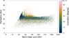 |
Fig. 1 Orbital distribution of semi-major axis and perihelion distance of planetesimals after 1 Gyr of evolution of giant planet migration. The colour coding indicates inclination. Data from Wong et al. (2023). |
Dynamical models overview.
2.2 Computing the satellite impact probabilities
There are two ways to calculate the impact probabilities of the planetesimals with the satellites (Ps). The first method makes use of the relative impact probabilities of the planetesimals on the satellites versus on the host planet and relies on an analytical approximation (Zahnle et al. 2003). We do not use that here.
The second method relies on numerical flyby simulations as detailed in Wong et al. (2019). We can express Ps as the fraction of planetesimals that collided on the satellites and multiply it by the probability of the planetesimals coming within 40 RP of a giant planet; we call the latter the encounter probability (Penc).
We have
 (1)
(1)
where Ni is the recorded number of impacts on the satellites, and Ntot is the total number of planetesimals that come with a distance of 40 RP. From the flyby simulations of the three planet-satellites systems, we could count the number of impacts on each regular satellite and calculate the absolute impact probabilities from which we can compute the impact rates.
2.3 Re-enacting the close encounters
For this work we decide to redo the flyby simulations using the CPU version of GENGA. The reason is the following.
Following Chambers (1999), the GENGA integrator computes a critical radius around each massive body in the simulation, whose magnitude is given by Rc =max(n1RH, n2υKh). Here RH is the Hill radius of the body, h is the time step, and n1 and n2 are constants set by the user; their default values are 3.0 and 0.4. For example, for Mercury using a time step of h = 0.01 yr we have Rc = 0.04 astronomical units (au) which is dominated by the second term, but for Jupiter with h = 0.4 yr we have Rc = 1.07 au which is dominated by the first term. Within this critical distance two bodies are considered to be within a close encounter, and the integration routine smoothly changes from the Mixed Variable Symplectic (MVS) map (Wisdom & Holman 1991) beyond Rc to the Bulirsch-Stoer routine (Grimm & Stadel 2014; Grimm et al. 2022) when the two bodies are closer than 0.2Rc. The changeover between the MVS and Bulirsch-Stoer regimes needs to be done smoothly so that during a close encounter the integrator should compute at least a few steps inside the changeover regime between 0.2 Rc and 1 Rc.
The default values of n1 = 3.0 and n2 = 0.4 in GENGA suffice for many problems: the value of n1 is identical to the default value in RMVS (Levison & Duncan 1994). It is typically sufficient for low-velocity encounters, or when the mass ratio between the central body and the planets or satellites is greater than O(10−5). However, when the masses are lower, the key distance factor is not the number of Hill radii, but rather the number of time steps used to sample the changeover region, in other words, the second term. A pair of objects with lunar mass can easily travel 3 mutual Hill radii in a single time-step. In this case the switch from the symplectic regime to the Bulirsch-Stoer regime is instantaneous, leading to large errors during the close encounter. As such, for high-velocity encounters, the n2 parameter becomes dominant (Chambers 1999).
The average encounter speed between the regular satellites of the giant planets and the hyperbolic heliocentric planetesimals can be computed with Pythagoras’ theorem, and is approximately  (Zahnle et al. 2003), so that within a time step the relative distance the satellite and a planetesimal travel is about
  . This distance is typically much greater than a few Hill radii of the satellites. As such, the n2 term dominates. It is likely that n2 = 0.4 is too low and the simulations may ‘step over’ close encounters as well as collisions between the satellites and the planetesimals. As such, we redid the simulations by setting n2 = 1. We reckon that this value is high enough because GENGA begins to check for potential close encounters at a distance of
  (in other words, at
  ).
).
Due to the low impact probabilities with the satellites it is necessary to re-enact many more encounters than are obtained during the giant planet migration simulations. We sampled the velocity distribution of the planetesimals as they penetrated the 40 planetary radii (RP) sphere, and recorded their values between 38 and 42 planetary radii. We created 25 000 massless planetesimals in this manner per simulation and ran 20 000 simulations per planet for a total of 500 million planetesimals per planet. Our maximum number of planetesimals per simulation was limited by computing time: higher numbers of planetesimals would increase the computing time more sharply than a linear increase due to greater RAM and CPU cache occupation. From testing we found that using 25 000 planetesimals using one CPU core gave excellent results, with each simulation lasting 12–17 seconds. In these flyby simulations all planetesimals passed by the satellites at once.
The isotropic initial position vectors of the planetesimals are computed according to
 (2)
(2)
where ξ1 and ξ2 are uniform random numbers in the interval [0, 1], and S is the distance to the planet corresponding to 40 RP. The angles θ and ϕ are the spherical latitude and longitude, respectively. The assumption of isotopic flybys has been validated by Zahnle et al. (1998) and the output from our GPU simulations confirm this. The velocities of the planetesimals are computed from angular momentum conservation and the requirement that they are initially all moving towards the planet. Their components are computed as
 (3)
(3)
where ξ3 and ξ4 are two additional uniform random numbers, u is the speed of the particle at 40 RP, whose magnitude and distribution was computed from the GENGA simulations, and ψ modulates the magnitude of the velocity vector components orthogonal to the direction towards the planet. With this prescription, the impact parameter of the planetesimals, b = L/u, where L is the specific angular momentum, is uniformly distributed in b2. Even though this impact parameter distribution is only strictly valid beyond 52 RU for Uranus, 75 RS for Saturn and beyond 110 RJ for Jupiter, this prescription does reproduce the trend from the GENGA planet migration simulations that Penc/PP ~ 50 (Wong et al. 2019). We computed the hyperbolic velocities at 40 RP from the migration and post-migration GENGA simulations in Wong et al. (2023), and from there calculated the encounter velocities ‘at infinity’ as  . For Jupiter 〈u〉 = 10.1 km s−1 leading to 〈υ∞〉 = 3.17 km s−1, for Saturn 〈u〉 = 6.85 km s−1 leading to 〈υ∞〉 = 3.65 km s−1, and for Uranus 〈u〉 = 4.25 km s−1 leading to 〈υ∞〉 = 2.39 km s−1.
For the purpose of our calculations, we assumed that the satellites reside on their present-day orbits. The initial positions and velocities of the Jovian, Saturnian, and Uranian satellites are from the JPL Horizons website. The time step was 0.01 days or 864 seconds and the maximum simulation time was just 20 days, by which time most of the planetesimals had left. With this time step Rc = 12000 km assuming υK = 14 km s−1 for Mimas, and GENGA will scan for encounters at a distance of at least 21 000 km, comparable to the relative distance travelled in a single time step between Mimas and a planetesimal, and will reduce the time step within this distance to the satellites. We therefore expect all collisions to be detected. For those few planetesimals that impacted a satellite their impact velocities were recorded.
3 Results and outcomes
3.1 Fundamental simulation parameters
Many small bodies in the trans-Neptunian region of the Solar System are on meta-stable orbits. These orbits could appear to be stable for billions of years because they are temporarily trapped in mean-motion resonances with Neptune (Duncan et al. 1995; Duncan & Levison 1997). Non-resonant objects with long semi-major axes whose perihelion lies within ~37 au evolve on billion-year timescales, undergoing a random walk in semi-major axis (Fernández et al. 2004), while resonant objects, once dislodged, can become Neptune crossing (Duncan et al. 1995; Duncan & Levison 1997). At short semi-major axis (often ≲100 au) secular effects are important, which alter the eccentricity, and thus the perihelion distance. These secular effects can flip a body from non-crossing to a crossing orbit, changing them from a scattered disc object to a Centaur or ecliptic comet. These combined dynamical effects cause a slow leakage of scattered disc and resonant objects into the Centaur region.
In order to compute the current impact rate onto the regular satellites we need to rely on the distribution of ecliptic comets, and more specifically on the injection rate of scattered disc objects into the realm of the giant planets. Ecliptic comets are scattered disc objects that have left their source region and become Neptune crossers; their motion is thus dominated by encounters with the planets, and by secular oscillations in inclination and eccentricity. A subset of these comets are the short-period Jupiter-family comets, which are concentrated along the ecliptic plane, and whose Tisserand parameter with respect to Jupiter T > 2 (Levison & Duncan 1997). The Tis-serand parameter with respect to a planet is akin to the Jacobi integral in the circular restricted three-body problem, and is roughly conserved during encounters with said planet. We qualified the particles in our simulations that met all the following criteria as an ecliptic comet (EC). Following Wong et al. (2023) our definition focuses on the EC injection rate, and not so much their actual fate. Our criteria are:
the planetesimal survived the first 1 Gyr during the migration episode;
its perihelion reached q < 30 au in the last 3.5 Gyr of the simulation, and
it is lost eventually due to collision with the planets or the Sun, ejection from the Solar System, or survived till the end of simulation at 4.5 Gyr.
As such, only those scattered disc objects that began to cross Neptune are counted as ecliptic comets.
Following Duncan et al. (1995) we computed the injection rate of ecliptic comets from the scattered disc as
 (4)
(4)
where NSD is the current number of objects in the scattered disc, rSD is the rate at which the scattered disc population declines, and fec is the fraction of scattered disc objects that become ecliptic comets. The rate of decline of scattered disc objects is computed as the number of planetesimals that left the system (ΔN) divided by the final number of the particles at the end (Nfin), and the time interval (Δt) (Duncan et al. 1995). In other words
 (5)
(5)
It is worth mentioning that rSD depends on the time range over which it is calculated because the rate of decline is not constant with time; instead, the rate of decline is a function of time itself: it decreases with increasing time. To approximate the current injection rate we calculated ΔN and Nfin over the last 0.5 Gyr in the simulations. Doing the same calculation over the last 1 Gyr increases the rate of decline by about 15%, and this increases to 50% if we consider the decline over the last 1.5 Gyr. These differences indicate the non-linearity of the rate of decline. We show this in Fig. 2, where we plotted the remaining percentage of the initial population over the last 3.5 Gyr from one of the GPU simulations. It is clear that the decline is much more rapid between 1 and 2 Gyr than between 3.5 and 4.5 Gyr. The fraction of bodies remaining after 4.5 Gyr is about 20% of the population at 1 Gyr, that is, the population declines by a further 80% between 1 Gyr and 4.5 Gyr of evolution. The percentage remaining after 1 Gyr of migration is typically 0.68% and therefore the total population remaining after 4.5 Gyr is 0.15%. Nesvorný et al. (2023) reports a remaining fraction of 0.25%.
Using Equation (5) to compute rSD is not without problems, however. The quantity ΔN changes discretely, and Poisson statistics dictate that the standard deviation  . If ΔN is a small quantity but Nfin is large, then the uncertainty in the ratio between different simulations, that is σrSD, will likely be low. But if Nfin is also a small quantity, with standard deviation
  , then both the ratio itself, and the uncertainty in the ratio ΔN/Nfin, can take on an (arbitrarily) large range in values due to stochastic variations in ΔN between different simulations. The expectation is that ΔN ≪ Nfin so that if ΔN is a low number σrSD ~ |rSD|(ΔN)−1/2 ~ |rSD| . As such, the expectation is that the uncertainties in rSD will become large when the number of remaining particles in the simulations and their rate of decline is low. These uncertainties cannot be reduced by running more simulations with the same initial number of particles.
To estimate the total number of ecliptic comets we need their mean dynamical lifetime, τEC. Levison et al. (2000) argue that
 (6)
(6)
where Ninit is the initial number of test particles, and N(s) is the number of test particles remaining at the time s < t. The last step is approximately valid because of the slow decline of planetesimals. The orbital elements or vectors of each body during the simulation are written to disk at regular time intervals: every 0.1 Myr for RMVS and every 0.3 Myr for GENGA. In this manner each simulation produced thousands of data frames. To compute τEC we, (a) searched each data frame for a particular particle, (b) determined whether its perihelion q < 30 AU, and then (c) counted the number of data frames the particle was in with q < 30 au. If its perihelion increased again beyond 30 au it was not counted. We computed τEC for each particle by multiplying the total number of data frames by the data output interval (either 0.1 or 0.3 Myr). We then averaged these individual times over all simulations per set to compute τEC.
The nominal average values of all of these quantities are listed in Table 2 for the different sets of numerical simulations that we performed. All the quantities derived from the simulations, as well as their uncertainties, are in the Supplementary Materials on Zenodo. In what follows we listed all the relevant quantities from all simulation sets, but for the analysis of the impact rate we used only the clone (C) simulations. The reason for this is that in the RMVS M simulations 〈∆N〉( = 1.34 so that σ∆N = 1.12 and the uncertainty in the rate of decline is σrSD ~ |rSD|, which is too great to derive a meaningful impact rate onto the giant planets.
We computed  Gyr−1 (2σ) from the RMVS C simulations, and rSD = −0.149 ± 0.004 Gyr−1 (1σ) from the combined GPU simulations. Most of our values fall in between those of previous literature estimates and their uncertainties from Brasser & Morbidelli (2013) (−0.163 ± 0.066), Fernández et al. (2004) (−0.15), Levison et al. (2006) (−0.27), Volk & Malhotra (2008) (−0.15 ± 0.05), but are much lower than that of Di Sisto & Brunini (2007) (−0.52). Some of these studies (Fernández et al. 2004; Di Sisto & Brunini 2007; Volk & Malhotra 2008) compute the injection rate from integrating the observed sample of then-known trans-Neptunian objects, while others (Levison et al. 2006; Brasser & Morbidelli 2013) rely on a distribution of planetesimals that results from long-term integrations of particles subjected to giant planet migration. The agreement between all these results is encouraging and suggests that the leakage rate may only be weakly dependent on the underlying orbital distribution of scattered disc objects.
From the RMVS C simulations we obtained  (2σ), and fEC = 78.7% ± 1.2% (1σ) from the GPU runs. The mean lifetime of the ecliptic comets in the RMVS clone simulations is
  Myr (2σ) and in the GENGA simulations the result is
  Myr (2σ). These large ranges are due to some simulation particles spending a long time on orbits only crossing one or both ice giants, for which the evolution timescale is of the order of 100 Myr (Duncan et al. 1987). We show examples of these long-lived particles in Fig. 3. We plotted the semi-major axis and perihelion distance of two particles that both survive the migration stage. The case displayed in orange spends a shorter time crossing Neptune as an EC than the black case. All of the average EC lifetimes listed above are comparable with that found by Levison et al. (2000), who report τEC = 190 Myr, but longer than found by Di Sisto & Brunini (2007) (72 Myr) and Tiscareno & Malhotra (2003) (9 Myr), but the last study only simulated ecliptic comets whose perihelia were close to Jupiter and Saturn, drastically reducing the dynamical lifetime.
For completeness we report that the total fraction remaining for the RMVS C simulations is  (2σ) and 0.15% ± 0.05% (1σ) for the GPU C simulations. Last, we report the fraction of the total population that are ECs with q < 30 au, which is computed as NEC = NSD |rSD|fECτEC. The mean and uncertainties were computed using a Monte Carlo sampling procedure from the underlying distributions in fEC, rSD, and τEC across all simulations in each set. For the RMVS C simulations we obtained
  Nsd (2σ), and
  Nsd (1σ) from the GPU simulations. The large uncertainties are almost entirely due to the distribution in τEC. Before we can calculate the current impact rate onto the giant planets and their satellites we need to know the number of scattered disc objects greater than some threshold diameter, NSD.
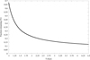 |
Fig. 2 Decline of the remaining fraction of planetesimals during the last 3.5 Gyr of dynamical evolution. The rate of decline slows down with increasing time. Data are from one of the GPU simulations of Wong et al. (2023). |
Nominal outcomes of numerical simulations.
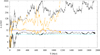 |
Fig. 3 Semi-major axis and perihelion distance evolution of two particles that survive for the first 1 Gyr. They spend a long (black) and short (orange) time on Neptune-crossing EC orbits. The blue and cyan lines indicate the semi-major axes of Neptune and Uranus, respectively. |
3.2 The current number of scattered disc objects and their size-frequency distribution
Based on Outer Solar System Origins Survey (OSSOS) observations the current estimated number of scattered disc objects with diameter Di > 10 km is (2.0 ± 0.8) × 107 (Nesvorný et al. 2019), assuming their albedo is 6%. We scaled the number of impactors from the observed number of scattered disc objects with Di. We have,
 (7)
(7)
Observations of distant scattered disc objects in the hot or excited population, as well as Jupiter’s Trojan asteroids, show that the slope α seems to have two values, one for objects with diameter Di ≳ 100 km, and another one for smaller objects (Shankman et al. 2013; Fraser et al. 2014; Lawler et al. 2018; Wong & Brown 2015; Yoshida & Terai 2017). These studies suggest that for Di ≳ 100 km |α1| = 4.5 ± 0.5 and for 1 ≲ Di ≲ 100 km objects |α2| = 2.0 ± 0.2. Wong et al. (2023) adopts the nominal values α2 = −2 and α1 = −4.5. For impactors with diameter Di < 1 km, we shall adopt the slope of Singer et al. (2019), in other words α3 = −0.7.
With the nominal adopted value of α2 by Wong et al. (2023) the expected current number of scattered disc objects with diameter Di > 1 km is approximately 2.0 × 10⁹, which is consistent within uncertainties with the values obtained by previous numerical and observational works (e.g. Brasser & Morbidelli 2013; Volk & Malhotra 2008; Shankman et al. 2013; Lawler et al. 2018). This estimate varies by at least a factor of three: Shankman et al. (2013) compute 2 × 10⁹ for Di > 1 .5 km (assuming an albedo of 4%), followed by Lawler et al. (2018), who increases it to 3 × 10⁹ for the same diameter. Volk & Malhotra (2008) report a number of 109, probably for objects with Di > 2 km (the exact diameter is not specified), and Brasser & Morbidelli (2013) estimate 2 × 10⁹ for Di > 2.3 km. It is possible that these studies adopt different size-frequency distributions at that size range, making scaling all of these values to Di > 1 km or Di > 10 km challenging. Can we verify whether any of the above estimates for NSD make sense?
One source of bodies that we can use are the Jupiter-family comets (JFCs). Following Levison & Duncan (1997) we can define the production rate of JFCs as rSDfJFC. Literature estimates show that fJFC = 16–30% (Levison & Duncan 1997; Di Sisto et al. 2009; Brasser & Morbidelli 2013). The usual reported number of active JFCs with diameter DJFC > 2 km and perihelion distance q < 2.5 au is 117 (Di Sisto et al. 2009). The dormant to active JFC ratio is about 5–6.5 (Levison & Duncan 1997; Di Sisto et al. 2009; Brasser & Morbidelli 2013), so to first order there are of the order of 700 dormant JFCs. These comets spend 7–10% of their dynamical life with q < 2.5 au (Brasser & Morbidelli 2013), so that there are about 104 JFCs with DJFC> 2 km in total. The median dynamical lifetime of these comets is 165 kyr (Levison & Duncan 1997; Brasser & Morbidelli 2013), so the loss rate is then approximately 0.06 yr−1. This must match the production rate NSDfJFC|rSD| and results in a nominal value of NSD = 2 × 10⁹ if we take fJFC = 20% and |rSD| = 0.15 Gyr−1, with a range of (1.1 - 2.5) × 109 accounting for the uncertainties of fJFC and |rSD|.
From their own analysis of numerical simulations of JFC production, Nesvorný et al. (2017) estimate that at present the number of active JFCs to scattered disc objects is 10−7 – comparable to 6.8 × 10⁻⁸ of Brasser & Morbidelli (2013) – and they compute that NSD = (1.5 – 4) × 107 with Di > 10 km, implying NSD = (1.5 – 4) × 109 with Di >1 km if α2 = −2, consistent on the lower end with earlier estimates. However, Nesvorný et al. (2017) assumes a physical lifetime of 500 orbits. In an independent study on near-earth objects including active JFCs Bottke et al. (2002) obtains NSD = (2.8 ± 2.0) × 109 objects beyond Neptune with Di > 1 km. However, most of the estimates for NSD derived from the JFC population pertain to objects with diameter Di > 2 km rather than 1 km, which agrees better with the estimates of Brasser & Morbidelli (2013); Shankman et al. (2013); Lawler et al. (2018) than with that calculated by us from the observational constraints by Nesvorný et al. (2019) and the numerical work by Nesvorný et al. (2017) for objects with Di > 10 km.
A potential problem presents itself when we extrapolate the estimate of the current population back in time before the onset of giant planet migration. The average depletion of the population in the clone simulations is 99.8%, comparable to the 99.7% of Nesvorný et al. (2017). If the current population with Di > 1 km is 2 billion, the original number was about 1012, which is higher than that computed by Nesvorný et al. (2023) and Wong et al. (2023) by a factor of 1.5, which is acceptable. But if the current population is 3 or 4 billion then it is difficult to reconcile with the original population unless its size-frequency distribution slopes are on the very steep end of what observational constraints allow.
One way out of this dilemma is to accept that the current population of scattered disc objects with diameter Di > 10 km is (2 ± 0.8) × 107 (Nesvorný et al. 2019) so that with our nominal depletion the nominal primordial population of such objects is 1010 – Nesvorný et al. (2017) reports (8 ± 3) × 109. With the primordial disc mass of 18 M⊕ from Wong et al. (2019, 2023), and adopting the knee size frequency distribution of trans-Neptunian objects from Fraser et al. (2014); Lawler et al. (2018) a primordial number of objects of 1010 with Di > 10 km requires that the size-frequency distribution slopes are either (α1; α2) = (5.0, 2.1) or (α1, α2) = (4.5, 2.2). In either case one of the slopes is at the higher end of literature estimates.
With these faint-end slopes and our depletion amount the current number of scattered disc objects with Di > 1 km becomes NSD = (2.5 – 3.2) × 109. In what follows we adopt a nominal value of NSD = 3 × 10⁹ for Di > 1 km. The resulting nominal number of ecliptic comets with Di > 1 km is then NEC = 5.4 × 10⁷ if we use the outcome of the GENGA simulations.
We now compute the ecliptic comet injection rate. From the RMVS clone simulations we obtain  yr−1 (2σ), while the combined GENGA simulations yield FEC = 0.353 ± 0.002 yr−1 (1σ) these estimates do not include the uncertainty in NSD. We resort to using the outcome of the GPU clone simulations, and we adopt a nominal value of FEC = 0.36 yr−1. With this approach the largest uncertainty in the impact rate is that from the number of scattered disc objects. In Table 3 we have listed the nominal values of all the relevant parameters that we adopted.
The nominal adopted values of several relevant simulation parameters.
Impact probabilities with the planets for different simulation sets.
Satellite impact rates and related quantities.
3.3 Impact probabilities with the giant planets and their satellites
The various impact probabilities of planetesimals with the giant planets and the satellites, as well as encounter probabilities with the planets, and impact speeds with the satellites are listed in Tables 4 and 5. The quantities derived from the numerical simulations, as well as their uncertainties, are given in the Supplementary Materials on Zenodo.
The first table lists the impact and encounter probabilities of planetesimals with the giant planets. The first two entries are obtained from the clone simulations run with GENGA for the last 3.5 Gyr (Wong et al. 2023). The third column is PP for the RMVS clone simulations. The next two columns are the same values as the first two, but are obtained from Wong et al. (2021) when the giant planets were migrating. The last column is the impact probability obtained from the RMVS M simulations. Even though the output from these last simulations is not used in our analysis, we list the impact probabilities here because our values are very similar to those of Levison et al. (2000) and these impact probabilities were used by Zahnle et al. (1998), and Zahnle et al. (2003) in their analysis of the current cratering rates.
Two things are of note. First, the impact probabilities with the planets after migration during the last 3.5 Gyr are lower than that during the migration phase, typically by a factor of 3–4. The reason is the different initial conditions of the migration and clone simulations. During the migration phase the planetesimals are located in a ring surrounding the outermost ice giant. They are excited by the migrating planets and are quickly scattered from one planet to another. During the last 3.5 Gyr most plan-etesimals from this initial ring are either ejected or collide with one of the giant planets. Planetesimals remaining after 1 Gyr of migration reside on meta-stable orbits (Duncan & Levison 1997) whose distribution is shown in Fig. 1, and their time-averaged orbital distribution is very different from the first 1 Gyr. The different initial conditions are also the reason why for Uranus Penc/PP < 40 in the M simulations. The reason is that during their migration a significant fraction of planetesimals encounter the ice giants on elliptic orbits, some of which are still recorded in the code as encounters if they venture close enough. For comparison, Zahnle et al. (1998) reports that 20% of planetesimals encounter Jupiter on elliptical orbits.
Second, the impact probabilities we computed with RMVS are systematically higher than with GENGA. The reason for this is likely to be the time step: we chose its value as a compromise between speed and accuracy, with the understanding that most planetesimals were ejected due to the cumulative effect of mostly distant encounters with the giant planets. However, with a large enough time step RMVS does not adequately resolve very close repeated encounters with the giant planets (Levison & Duncan 1994; Michel & Valsecchi 1996), while GENGA, using a Bulirsch-Stoer integrator close to the planet, likely does a better job of resolving such close encounters. The impact probability difference between RMVS and GENGA is a factor of 1–1.5, which is propagated into the impact rates. In what follows we adopt the impact probabilities from the GENGA simulations.
Table 5 contains the impact probabilities of planetesimals with the satellites. The first entry, Ps/PP, is the impact probability scaled to that of the planet obtained from our flyby simulations, where we counted the number of impacts on a satellite and divided by the number that hits the planet. The next entry, Ni/Ntot, is the impact probability of a planetesimal that ventures within 40 RP as computed from our flyby simulations This is the number of planetesimals that collide with a satellite divided by the total number of planetesimals (500 million) in the flyby simulations. The next entry, Ps is the absolute impact probability of a heliocentric planetesimal with the satellites, and is computed as Ni/Ntot × Penc, where we used the Penc values on the planets from the GENGA simulations during the last 3.5 Gyr. As an example, for Enceladus Ni/Ntot = 0.10 × 10⁻⁶, suggesting that typically we recorded 50 impacts out of 500 million particles in the flyby simulations, and Penc = 5.95% for Saturn so that the absolute impact probability becomes Ps = 0.1 × 10−6 × 0.060 = 0.60 × 10⁻⁸, which is a little lower than using the relation Ps/PP × PP. The discrepancy between these two values of the absolute impact probability is largest for Mimas and Enceladus. This could be attributed to the flyby simulations missing some encounters and impacts due to the high encounter speeds with these tiny bodies, but several iterations of the flyby simulations with higher values of n2 > 1 did not remedy that problem. We subsequently list the average impact speed with the satellite obtained from the flyby simulations, followed by the impact rate of objects with Di > 1 km, and the crater diameter that such an impact produces. The last entry is cratering rate for craters with diameter Dcr > 10 km assuming the crater scaling relations discussed below.
We note that the differences between Ps/PP and with direct hits during the flyby simulations are typically 30% and are smallest for the Jovian satellites Io, Europa, and Ganymede (about 10%). We do not know what accounts for this large difference. Both the analytical estimate of Zahnle et al. (2003) and our numerical flyby simulations have their own assumptions and limitations, but Zahnle et al. (2003) did say that their Monte Carlo procedures gave results that were 30% different from their analytical solutions. Additional differences could result from numerical factors in the flyby simulations and the fact that the gravitational focusing of the giant planets becomes important for Saturn and Uranus at closer distances than for Jupiter, resulting in a different initial distribution of the impact parameter. The uncertainty in the value of PP is at least a factor of 1.3.
3.4 Current impact rate on the satellites
We computed the current impact rate on a satellite (or a planet) following the procedure from Duncan et al. (1995) and Levison et al. (2000) based on the injection rate (FEC) of ecliptic comets with Di ≥ 1 km originating from beyond Neptune, and on the impact probability with the satellites with the giant planets. The formula for calculating the impact rate is
 (8)
(8)
where Ps is the post-migration collision probability onto a satellite as described in Equation (1).
The impact rates listed in the fifth column of Table 5 need to be converted into a cratering rate using crater scaling laws to convert impactor diameter to craters, and vice versa. Wong et al. (2023) employs a crater scaling law based on the π-scaling law, using the simple-to-complex crater diameter relation DSC = 4 (1 ms−2/ɡ) km (Schenk 1991), which applies to all icy satellites apart from Mimas, Enceladus, Tethys, Dione, and Miranda, for which DSC ~ 15 km (Schenk 1991). For Io, DSC = 24 (1 m s−2/ɡ) km (Pike 1980). The crater scaling law in Wong et al. (2023) for icy bodies is
 (9)
(9)
where the bottom equation applies to Mimas, Enceladus, Tethys, Dione and Miranda, and the top equation to the other satellites (for Io the coefficient in the top equation is 3.39). For both crater scaling laws we assume that the impact angle is 45°. These scaling laws are somewhat different from those in Zahnle et al. (2003). Wong et al. (2023) assumes an impactor density of ρi = 400 kg m−3, which is the mean density of comet Tempel 1 (Richardson et al. 2007) and which is a little lower than that of Churyumov-Gerasimenko (Jorda et al. 2016), and a satellite density ρs = 1000 kg m−3 apart from Io, for which ρs = 3520 kg m−3. We employ values for the traditional scaling parameters α = 0.85, which describes the simple-to-complex crater diameter ratio (Croft 1985), and β = 0.22, which relates the efficiency of crater excavation in the gravity-dominated regime. The inverse relations for icy bodies are
 (10)
(10)
from which we compute the cratering rate for Dcr > 10 km using the inferred impactor size-frequency distribution slope of α3 = −0.7 for impactors with Di < 1 km (Singer et al. 2019), and following Nesvorný et al. (2019) by adopting α2 = −2.1 for Dimp > 1 km. The uncertainties in the cratering rate are a factors of a few, primarily due to uncertainties in FEC (including in NSD). For Io the coefficient of the top equation becomes 0.264.
The nominal value of FEC and the current impact probability of Jupiter result in a rough estimation of the impact rate on Jupiter, which we compute as 1.0 × 10⁻³ per year for objects with Di > 1 km. Our estimated Jovian impact rate falls towards the low end, but remains consistent with values from previous studies. The ranges and uncertainty of impact rates in Zahnle et al. (2003) are discussed in Section 4, but suffice to say that the range of these impact rates for Di > 1 km spans two orders of magnitude, and the uncertainties in these estimates also vary. We also calculated the impact and cratering rates on Enceladus (and the other satellites of all three planets). The impact rate of objects with Di > 1 km with Enceladus is computed to be 2.12 Gyr−1. For the cratering rate we used the inverse crater scaling law. With our adopted values for the impactor density, satellite density, and impact velocity from Table 5, a crater with diameter Dcr > 10 km on Enceladus requires a projectile diameter of Di = 0.41 km and adopting the size-frequency distribution slope α3 = −0.7 from Singer et al. (2019) the current cratering rate becomes 5.0 × 10⁻⁶ km−2 Gyr−1.
Impact rates and cratering rates on the giant planets and Enceladus from various dynamical models.
4 Comparison with earlier work
We present three sets of studies that estimate current impact rates and surface age for the icy satellites. These sets include:
Classic studies (Zahnle et al. 1998, 2003; Kirchoff & Schenk 2009),
Recent studies by others (Nesvorný et al. 2019, 2023; Bottke et al. 2023, 2024), and
Recent studies by us (Wong et al. 2019, 2021, 2023), and this work.
Each group of studies represents a series of works that begin with planetary dynamics and impact rate estimations, progressing towards determining crater ages for the icy satellites. These works employ various methodologies and sources, ranging from numerical simulations of planetary migration to observational crater counts. It is important to note that no single paper in any of these sets comprehensively addresses the entire spectrum from planetary dynamics to geological history.
We shall discuss the differences in results from the three studies by listing the impact rates on Jupiter and Enceladus, and the cratering rate on the latter, in Table 6. In the following, we address the large uncertainties and differences between our impact rate estimates, and those from previous studies.
4.1 Classic studies
Zahnle et al. (1998, 2003) constrain the current impact rate on Jupiter through multiple measurements. Zahnle et al. (2003) reports an impact rate of approximately 4 × 10⁻³ yr−1 based on six encounters (smallest ~1 km in diameter) within four Jovian radii over ~350 years. Lamy et al. (2004) observe nine comets crossing Callisto’s orbit over approximately 50 years, suggesting an impact rate of about 1.75 × 10⁻³ per year for Di > 1 km. Other estimations, using recorded collisions and close encounters, measurements of excess carbon monoxide content, crater counting on Ganymede, and inference from Near Earth Objects, range from 0.4 to 44 × 10−3 impacts per year. The ranges Zahnle et al. (2003) discusses are: historical records (4.3 × 10⁻³ to 2.3 × 10⁻² impacts per year), observed impacts (1.4 × 10⁻² to 4.4 × 10⁻² yr−1), excess carbon monoxide content (7.7 × 10⁻³ yr−1), crater counting on heavily cratered terrain on Ganymede (2.0 × 10⁻³ to 4.8 × 10⁻² yr−1), and inferred impacts from Near Earth Objects (1.3 × 10⁻³ yr−1). All impact rates above are scaled to impactors with diameters Di > 1 km, assuming a cumulative power-law slope of α2 = −2 (Singer et al. 2019). In any case, the impact rate on Jupiter of Zahnle et al. (1998, 2003) have uncertainties that vary significantly, ranging from a factor of three to an order of magnitude. Zahnle et al. (2003) calibrate the impact rate on Jupiter at  yr−1 for impactors with Di > 1 .5 km.
This commonly cited Jovian impact rate for Di ≥ 1 .5 km, when translated using their Case A size-frequency distribution, corresponds nominally to 10−4 yr−1 for impactors with diameter Di ≥ 10 km, and 7.5 × 10⁻³ yr−1 for Di ≥ 1 km. Using α2 = −2.1 we find similar results: 9.3 × 10⁻⁵ yr−1 for Di ≥ 10 km, and 1.0 × 10⁻² yr−1 for Di ≥ 1 km. We note that Case A of Zahnle et al. (2003) represents a shallower size-frequency distribution of the impactors, with α3 = −1 for Di < 1.5 km, whereas their Case B reflects a steeper distribution closer to a collisionally evolved population deduced from craters on Triton (α3 = −2.5 for Di < 1.5 km). Most recent studies adopt Case A as a more accurate representation of heliocentric comet populations in the outer Solar System, so that we shall do the same. The shallow slope is also more closely aligned with the results of Singer et al. (2019).
Zahnle et al. (2003) theoretically assess the impact rate on Saturn by considering several factors: the proportion of comets delivered from beyond Neptune’s orbit to Jupiter’s, the impact probability based on the planets’ relative sizes to their Hill spheres, and the gravitationally enhanced cross-sections, which are proportional to each planet’s mass and escape velocity. From this, they estimate the impact ratio of Jupiter to Saturn to be 1:0.42. This is close to the ratio of 1:0.47 from the average annual Öpik impact probabilities for the three then-known Centaurs with Saturn, for which the impact rate is computed as 2 × 10⁻⁸ yr−1 for a 150 km diameter object (Fernández et al. 2002). Together, this corresponds to a Saturnian impact rate of 3.2 × 10⁻³ yr−1 for Di ≥ 1 km, using the Case A size-frequency distribution.
With this information we compute that the current impact rate on Enceladus, scaled from Jupiter and using Case A, is approximately 16.7 Gyr−1 for objects with Di > 1 km. We used Ps/PP = 2.2 × 10⁻⁶ for the Enceladus to Jupiter impact probability ratio, and that the impact rate on Jupiter is 5 × 10⁻³ yr−1 for Di ≥ 1 .5 km. This impact rate on Enceladus is a factor of eight higher than our estimate, and is primarily due to Zahnle et al. (2003) taking a factor of six higher impact rate on Jupiter, as well as our different size-frequency distribution between impactor diameters 1 km and 1.5 km. To compute the cratering rate on Enceladus we use the inverse of the crater scaling laws adopted by Zahnle et al. (2003) (see the Appendix). Using the impact velocity of heliocentric planetesimals with Enceladus listed by Zahnle et al. (2003) of υi = 24 km s−1 the impactor diameter required to excavate a crater with diameter Dcr > 10 km on Enceladus is Di = 0.34 km. Adopting the Case A size-frequency distribution implies the current impact rate of such planetesimals on Enceladus is 49 Gyr−1. The resulting cratering rate is then 6.1 × 10⁻⁵ km−2 Gyr−1, which is a factor of 12 greater than our estimate, with the additional factor of two over the impact rate being caused by our different adopted crater scaling law and slope.
4.2 Recent studies
In the last five years, Nesvorný et al. (2023) have built upon their earlier works of Nesvorný (2015a,b); Nesvorný et al. (2017) to further constrain the initial conditions of the giant planet migration model, specifically the initial semi-major axis of Neptune and its migration pathway. The most recent version of the model assumes that the dynamical instability among the giant planets occurred 10 Myr after the dispersal of the protoplanetary gas disk. The migration rate of Neptune follows an exponential profile (Nesvorný et al. 2017): for the first 10 Myr, the migration e-folding time (τ) is 10 Myr, representing rapid migration. Then, after 10 Myr of dynamical evolution, τ increases to 30 Myr, reflecting a slower migration rate, which lasts up to 500 Myr.
Nesvorný et al. (2023) uses the initial conditions of the simulations of Nesvorný et al. (2017) and reran the last 1 Gyr of evolution. They begin with one million test particles from Nesvorný et al. (2017) and apply ‘on-the-fly’ cloning when any particle ventures closer than 23 AU for the first time, cloning it 50 times to maintain sufficient particle interactions with the planets.
From the simulation’s impact counts, Nesvorný et al. (2023) calculates the impact rate on Jupiter as 3.5 × 10⁻⁵ per year for objects with Di ≥ 10 km, without considering cometary disruption. They compute the impact rate as Ċp = (Δn/t) (nimp/ntp), where T is 1 Gyr, and ΔN is essentially equal to the original number of planetesimals in the disc because 99.7% are lost (Nesvorný et al. 2017). In Nesvorný et al. (2023) they adopt ΔN = (8 ± 3) × 109 with Di > 10 km and they record Nimp = 217 impacts on Jupiter out of a total of Ntp = 5 × 10⁷ test particles; in this manner they obtain their nominal value Ċp = 3.5 × 10⁻⁵ per year. With cometary disruption included, the rate decreases to 2.6 × 10⁻⁵ yr−1. Using their adopted impactor power-law slope of α2 = −2.1, we computed that their impact rate on Jupiter for Di > 1.5 km becomes 1.9 × 10⁻³ yr−1 without disruption, and 1.4 × 10⁻³ yr−1 with disruption. These values are still higher than ours by factors of a few, but they also fall outside the range of  yr−1 of Zahnle et al. (2003). The impact rates for objects with Di > 1 km are listed in Table 6.
To calculate the collision probability with Enceladus, Nesvorný et al. (2023) record the close encounters within a Hill radius of Saturn and numerically evaluate the collision probability for each Saturnian encounter with Enceladus. Following Zahnle et al. (2003) the impact rate was then scaled to that of Jupiter. Using their nominal impact rate on Jupiter of 3.5 × 10⁻⁵ yr−1 for Di ≥ 10 km and Ps/Pp = 1.5 × 10⁻⁶ as the Enceladus to Jupiter impact probability ratio – see Table 2 of Nesvorný et al. (2023) – the impact rate on Enceladus becomes 0.053 Gyr−1 for Di > 10 km, and 6.6 Gyr−1 for Di > 1 km using α2 = −2.1; this impact rate is a factor of 2.5 higher than our value.
Nesvorný et al. (2023) do not explicitly compute the crater-ing rate onto the satellites, only the relative impact probabilities. Since some of their methodology follows that of Zahnle et al. (2003) we can naively adopt the same cratering scaling law as Zahnle et al. (2003) and the size-frequency distribution of their Case A for objects with diameter Di < 1 km. We then computed the cratering rate on Enceladus as 2.4 × 10⁻⁵ km−2 Gyr−1 for the non-disruption case, and 2.2 × 10⁻⁵ km−2 Gyr−1 with disruption. These cratering rates are a factor of three to four higher than ours and a factor of three to four lower than that of Zahnle et al. (2003).
5 Discussion
In this section we discuss our results in comparison to previous studies in more detail. To begin, we find that the impact rates onto Jupiter and Enceladus, and by extension the other giant planets and their satellites, is lower than that found by two other studies. We made our methodology transparent, we clarified every choice of every parameter and how they were used. It is strange that despite many of these parameters being similar to some of the previous studies, we still find a very different impact rate. Why is this so? There are several reasons that we can think of.
The first is the outcome of the numerical simulations. The migration simulations in Wong et al. (2023) move Neptune and Uranus out slower than Nesvorný et al. (2017), but Nesvorný et al. (2023) concluded that the details of the migration should not matter for the current impact rates. We concur with this statement based on logical deduction alone. However, Wong et al. (2023) find that the location of the planetesimal disc’s outer edge appears to play a role because it influences the depletion, fraction that becomes ecliptic comets, and the rate of decay, but only when the outer edge is beyond 35 au. Furthermore, the migration occurs very early and the outer Solar System is relatively stable for the past 3.5 Gyr. Therefore the current impact rate – which reflects only the most recent few hundred Myr – should not strongly depend on the specific details of Neptune’s migration, such as its speed or timing if it occurred more than 4 Gyr ago. The adopted disc mass and its width by Wong et al. (2023) are also comparable to Nesvorný et al. (2017), and we obtained the same amount of depletion by 4.5 Gyr of evolution, apart from cases where the disc extended beyond 35 au. The average rate of decline of our scattered disc population is consistent with other works in the literature. If this parameter is fundamentally wrong in our simulations it has to be equally wrong in others; this is highly unlikely. Unfortunately we do not have the numerical resolution to determine fJFC , and other studies do not report fEC so that we cannot compare our values to the works of others; the only parameter with which we can do this is rSD, which agrees across the board.
One difference between the outcome of our numerical simulations, that of Levison & Duncan (1997), and Levison et al. (2000) is that our impact probability with the planets is lower than in these studies, even though the impact probability for the simulations with migration are comparable to those in Levison et al. (2000). Levison & Duncan (1997) do not explicitly report the impact probabilities, yet the simulations of Levison et al. (2000) also find a comparable lifetime for the ecliptic comets than we do, once again lending credibility to our approach. We argued why our clone simulations are a good proxy for the current population and why the impact probabilities from this population should be considered rather than that including the migration; simply put: the migration phase is not a good proxy for the current solar system. In our studies, we derive the impact probability probabilities of the satellites by multiplying the impact count during the flyby simulations with the encounter probability with the planets. Both counts were recorded in dynamic simulations. Nesvorný et al. (2023), however, numerically evaluates the collision probability of each planetesimal encounter with the giant planets and its satellites, yet we find similar impact probability ratios Ps/PP to Zahnle et al. (2003) and Nesvorný et al. (2023), so that our different approach still yields consistent results.
A second potential reason for disagreement is the current number of scattered disc objects that we use. Neither Zahnle et al. (2003) nor Nesvorný et al. (2023) explicitly mention this number because they have no need for it. Unfortunately this quantity is poorly known and it will probably remain so for the time being. We made clear why we have chosen the number that we did, based on constraints from the total depletion of the population of planetesimals in our simulations as well as constraints on the primordial disc mass and the observed slopes of the size-frequency distribution of these objects, and the observational constraints. We do not foresee that the current population can be much more or much less numerous than what we have used here; factors of two perhaps. As such, this quantity is perhaps also not to blame.
A third possibility of disagreement is the choice of impactor size-frequency distribution. Our choices are certainly different from those of Zahnle et al. (2003) and partially accounts for our lower impact rates, but we deliberately choose the same slope of α2 = −2.1 as Nesvorný et al. (2023) for objects with diameter 1 ≲ Di ≲ 100 km to minimise differences in outcome. We extended the population to sub-km objects by adopting α3 = −0.7 from Singer et al. (2019), but if we restrict ourselves to computing the impact rate of km-sized objects then this choice does not matter. Thus, our difference of a factor of a few with Nesvorný et al. (2023) cannot be explained by the choice of impactor size-frequency distribution slope.
Beyond these relatively obvious potential differences that all yield comparable outcomes, there is one additional divergence in impact rate calculation methods that could contribute to the observed discrepancies in our results: the fundamental difference in approach. Both Zahnle et al. (2003) and Nesvorný et al. (2023) anchor their satellites’ impact rate to that of Jupiter. Whether this is derived from simulations or from observational constraints is less relevant. The satellite-to-Jupiter impact probability ratio and Jupiter’s absolute impact rate yield the resulting satellites’ impact rate. While the impact probability with satellites is implicit in this method, it is indirectly informed by the impact probability with Jupiter, even if this is not explicitly stated in Zahnle et al. (2003).
In contrast, our approach uses the flux of new comets entering the Centaur region from beyond Neptune as the fundamental parameter. This is then multiplied by the absolute impact probability with the satellites – derived from flyby simulations and the encounter probabilities with the giant planets – to yield the satellites’ impact rate. This is where the major differences show up: our impact rate on Jupiter is a factor of eight lower than that of Zahnle et al. (2003), and at least three lower than that of Nesvorný et al. (2023). The discrepancy with Zahnle et al. (2003) is primarily due to their choice of fixing the impact rate on Jupiter from historical observations rather than numerical simulations, while the discrepancy with Nesvorný et al. (2023) is more difficult to explain, but it appears to be due to how they compute the impact rate on Jupiter over the last billion years for objects with Di > 10 km, and their potentially anomalously low impact probability with this planet.
As a thought experiment we may use the impact rate on Jupiter adopted by Zahnle et al. (2003) at face value and compute what the injection rate of comets with Di > 1 km from beyond Neptune needs to be to be consistent with this impact rate. We obtain FEC = 2.6 yr−1. For this high value there is no literature precedent. Even if we were to adopt an impact probability with Jupiter of about 1% (Levison et al. 2000) rather than our value of 0.29%, the injection rate still needs to be 0.75 yr−1, which is still very high. Repeating this check for the impact rate of Nesvorný et al. (2023) with our impact probability and without disruption results in 1.5 yr−1, for which there is also no literature precedent either; using the higher impact probability on Jupiter of 1% lowers this to 0.44 yr−1, which is acceptable, but this cannot be verified without knowing their impact probability with Jupiter.
One potential effect that we did not consider is tidal disruption of comets. From crater chains on Ganymede and Callisto, and assuming their surfaces ages are about 4 Gyr old, Schenk et al. (1996) argue that there are 3.7 × 10⁻³ tidal disruptions per year near Jupiter. Since these disruptions generally happen within 3 RJ for comets with Di ~ 1 km this rate of disruption is fairly consistent with our estimated impact rate on Jupiter, yet with typically 10 fragments generated these disruptions are insufficient to elevate the impact rate at Jupiter by a factor of a few.
6 Conclusions
In this work, we uses numerical simulations of the evolution of the outer Solar System to compute the impact and cratering rates onto the regular satellites of Jupiter, Saturn, and Uranus, highlighting the complexities involved in determining these rates. We demonstrated how the current impact rate depends strongly on the specific parameters of the dynamical and disc models employed.
We outlined our methodology and parameter choices in detail, allowing future studies to verify or adjust these assumptions and recalculate impact rates. After careful comparison with previous works, we conclude that our impact rates are lower than that the best estimates of previous studies by up to a factor of six, likely due to our reliance on the injection rate of scattered disc objects into the Centaur region rather than anchoring to the impact rate on Jupiter. This difference in both approach and outcome highlights the importance of clearly stating all parameters and assumptions in future studies to enable meaningful comparisons.
Our findings underscore that the uncertainties in impact rates substantially influence surface age estimates, particularly for young, sparsely cratered terrains such as Europa, Enceladus, and young patches on Tethys and Dione. Better constraints on orbital dynamics and impactor size-frequency distributions are needed to refine both current and historical impact rates.
Future advances, such as more precise measurements of small body sizes using stellar occultation techniques, can provide crucial data to constrain the current impact rates and improve our understanding of the historical evolution of small bodies in the outer Solar System. These insights will help bridge gaps between impact dynamics and geological interpretations of icy moon surfaces.
Data availability
Supplementary materials are available on https://doi.org/10.5281/zenodo.14974372
Acknowledgements
This study is supported by the Research Council of Norway through its Centres of Excellence funding scheme, project No. 332523 PHAB. GENGA can be obtained from Bitbucket.
Appendix A Crater scaling
Zahnle et al. (2003) uses the following crater scaling law

where ɡ is the acceleration due to gravity, ρi and ρt are the densities of the impactor and the satellite, and DSC is the simple to complex transition crater diameter. Zahnle et al. (2003) uses DSC = 2.5 km for Europa, Ganymede, Callisto, and Titan (Schenk et al. 2004) and DSC = 15 km for all other satellites as well as an impactor density of ρi = 600 kg m−3 and a satellite density of ρs = 900 kg m−3 for all satellites apart from Io, for which ρs = 2700 kg m−3. The top equation should be applied when Dcr < DSC. The inverse equations are then

References
- Bottke, W. F., Morbidelli, A., Jedicke, R., et al. 2002, Icarus, 156, 399 [NASA ADS] [CrossRef] [Google Scholar]
- Bottke, W. F., Vokrouhlický, D., Marschall, R., et al. 2023, PSJ, 4, 168 [NASA ADS] [Google Scholar]
- Bottke, W. F., Vokrouhlický, D., Nesvorný, D., et al. 2024, PSJ, 5, 88 [Google Scholar]
- Brasser, R., & Morbidelli, A. 2013, Icarus, 225, 40 [Google Scholar]
- Chambers, J. E. 1999, MNRAS, 304, 793 [Google Scholar]
- Croft, S. K. 1985, Lunar Planet. Sci. Conf. Proc., 90, C828 [Google Scholar]
- Di Sisto, R. P., & Brunini, A. 2007, Icarus, 190, 224 [Google Scholar]
- Di Sisto, R. P., Fernández, J. A., & Brunini, A. 2009, Icarus, 203, 140 [Google Scholar]
- Duncan, M. J., & Levison, H. F. 1997, Science, 276, 1670 [Google Scholar]
- Duncan, M., Quinn, T., & Tremaine, S. 1987, AJ, 94, 1330 [Google Scholar]
- Duncan, M. J., Levison, H. F., & Budd, S. M. 1995, AJ, 110, 3073 [NASA ADS] [CrossRef] [Google Scholar]
- Fernandez, J. A., & Ip, W. H. 1984, Icarus, 58, 109 [NASA ADS] [CrossRef] [Google Scholar]
- Fernández, Y. R., Jewitt, D. C., & Sheppard, S. S. 2002, AJ, 123, 1050 [Google Scholar]
- Fernández, J. A., Gallardo, T., & Brunini, A. 2004, Icarus, 172, 372 [CrossRef] [Google Scholar]
- Fraser, W. C., Brown, M. E., Morbidelli, A., Parker, A., & Batygin, K. 2014, ApJ, 782, 100 [Google Scholar]
- Grimm, S. L., & Stadel, J. G. 2014, ApJ, 796, 23 [NASA ADS] [CrossRef] [Google Scholar]
- Grimm, S. L., Stadel, J. G., Brasser, R., Meier, M. M. M., & Mordasini, C. 2022, ApJ, 932, 124 [NASA ADS] [CrossRef] [Google Scholar]
- Holman, M. J., & Wisdom, J. 1993, AJ, 105, 1987 [NASA ADS] [CrossRef] [Google Scholar]
- Jorda, L., Gaskell, R., Capanna, C., et al. 2016, Icarus, 277, 257 [Google Scholar]
- Kirchoff, M. R., & Schenk, P. 2009, Icarus, 202, 656 [Google Scholar]
- Lamy, P. L., Toth, I., Fernandez, Y. R., & Weaver, H. A. 2004, in Comets II, eds. M. C. Festou, H. U. Keller, & H. A. Weaver (Tucson: University of Arizona Press), 223 [Google Scholar]
- Lawler, S. M., Shankman, C., Kavelaars, J. J., et al. 2018, AJ, 155, 197 [NASA ADS] [CrossRef] [Google Scholar]
- Levison, H. F., & Duncan, M. J. 1994, Icarus, 108, 18 [NASA ADS] [CrossRef] [Google Scholar]
- Levison, H. F., & Duncan, M. J. 1997, Icarus, 127, 13 [Google Scholar]
- Levison, H. F., Duncan, M. J., Zahnle, K., Holman, M., & Dones, L. 2000, Icarus, 143, 415 [NASA ADS] [CrossRef] [Google Scholar]
- Levison, H. F., Duncan, M. J., Dones, L., & Gladman, B. J. 2006, Icarus, 184, 619 [Google Scholar]
- Levison, H. F., Morbidelli, A., Van Laerhoven, C., Gomes, R., & Tsiganis, K. 2008, Icarus, 196, 258 [Google Scholar]
- Michel, P., & Valsecchi, G. B. 1996, Celest. Mech. Dyn. Astron., 65, 355 [Google Scholar]
- Nesvorný, D. 2015a, AJ, 150, 73 [CrossRef] [Google Scholar]
- Nesvorný, D. 2015b, AJ, 150, 68 [CrossRef] [Google Scholar]
- Nesvorný, D., Vokrouhlický, D., Dones, L., et al. 2017, ApJ, 845, 27 [CrossRef] [Google Scholar]
- Nesvorný, D., Vokrouhlický, D., Stern, A. S., et al. 2019, AJ, 158, 132 [Google Scholar]
- Nesvorný, D., Dones, L., De Prá, M., Womack, M., & Zahnle, K. J. 2023, Planet. Sci. J., 4, 139 [Google Scholar]
- Pike, R. J. 1980, Lunar Planet. Sci. Conf., 11, 2159 [Google Scholar]
- Richardson, J. E., Melosh, H. J., Lisse, C. M., & Carcich, B. 2007, Icarus, 190, 357 [Google Scholar]
- Schenk, P. M. 1991, J. Geophys. Res., 96, 1887 [NASA ADS] [Google Scholar]
- Schenk, P. M., Asphaug, E., McKinnon, W. B., Melosh, H. J., & Weissman, P. R. 1996, Icarus, 121, 249 [Google Scholar]
- Schenk, P. M., Chapman, C. R., Zahnle, K., & Moore, J. M. 2004, Ages and Interiors: the Cratering Record of the Galilean Satellites, eds. F. Bagenal, T. E. Dowling, & W. B. McKinnon (Cambridge: Cambridge University Press), 1, 427 [Google Scholar]
- Shankman, C., Gladman, B. J., Kaib, N., Kavelaars, J. J., & Petit, J. M. 2013, ApJ, 764, L2 [Google Scholar]
- Singer, K. N., McKinnon, W. B., Gladman, B., et al. 2019, Science, 363, 955 [NASA ADS] [CrossRef] [Google Scholar]
- Tiscareno, M. S., & Malhotra, R. 2003, AJ, 126, 3122 [NASA ADS] [CrossRef] [Google Scholar]
- Volk, K., & Malhotra, R. 2008, ApJ, 687, 714 [Google Scholar]
- Wisdom, J., & Holman, M. 1991, AJ, 102, 1528 [Google Scholar]
- Wong, I., & Brown, M. E. 2015, AJ, 150, 174 [NASA ADS] [CrossRef] [Google Scholar]
- Wong, E. W., Brasser, R., & Werner, S. C. 2019, Earth Planet. Sci. Lett., 506, 407 [CrossRef] [Google Scholar]
- Wong, E. W., Brasser, R., & Werner, S. C. 2021, Icarus, 358, 114184 [NASA ADS] [CrossRef] [Google Scholar]
- Wong, E. W., Brasser, R., Werner, S. C., & Kirchoff, M. R. 2023, Icarus, 406, 115763 [Google Scholar]
- Yoshida, F., & Terai, T. 2017, AJ, 154, 71 [NASA ADS] [CrossRef] [Google Scholar]
- Zahnle, K., Dones, L., & Levison, H. F. 1998, Icarus, 136, 202 [NASA ADS] [CrossRef] [Google Scholar]
- Zahnle, K., Schenk, P., Levison, H., & Dones, L. 2003, Icarus, 163, 263 [NASA ADS] [CrossRef] [Google Scholar]
All Tables
Impact rates and cratering rates on the giant planets and Enceladus from various dynamical models.
All Figures
|
Fig. 1 Orbital distribution of semi-major axis and perihelion distance of planetesimals after 1 Gyr of evolution of giant planet migration. The colour coding indicates inclination. Data from Wong et al. (2023). |
| In the text | |
|
Fig. 2 Decline of the remaining fraction of planetesimals during the last 3.5 Gyr of dynamical evolution. The rate of decline slows down with increasing time. Data are from one of the GPU simulations of Wong et al. (2023). |
| In the text | |
|
Fig. 3 Semi-major axis and perihelion distance evolution of two particles that survive for the first 1 Gyr. They spend a long (black) and short (orange) time on Neptune-crossing EC orbits. The blue and cyan lines indicate the semi-major axes of Neptune and Uranus, respectively. |
| In the text | |
Current usage metrics show cumulative count of Article Views (full-text article views including HTML views, PDF and ePub downloads, according to the available data) and Abstracts Views on Vision4Press platform.
Data correspond to usage on the plateform after 2015. The current usage metrics is available 48-96 hours after online publication and is updated daily on week days.
Initial download of the metrics may take a while.