| Issue |
A&A
Volume 535, November 2011
|
|
|---|---|---|
| Article Number | A102 | |
| Number of page(s) | 4 | |
| Section | Stellar structure and evolution | |
| DOI | https://doi.org/10.1051/0004-6361/201117852 | |
| Published online | 18 November 2011 | |
Research Note
No apparent accretion mode changes detected in Centaurus X-3
1
Institut für Astronomie und Astrophysik, Universität Tübingen, Sand 1, 72076 Tübingen, Germany
e-mail: daniela.mueller@astro.uni-tuebingen.de
2
MAXI team, RIKEN, 2-1 Hirosawa, Wako, Saitama 351-0198, Japan
Received: 8 August 2011
Accepted: 30 September 2011
Aims. Two distinct spectral states have previously been reported for Cen X-3 on the basis of RXTE/ASM observations. Intrigued by this result, we investigated the spectral properties of the source using the enhanced possibilities of the X-ray data now available with the aim to clarify and interpret the reported behavior.
Methods. To check the reported results, we used the same data set and followed the same analysis procedures as in the work that reported the two spectral states. Additionally, we repeated the analysis using the enlarged data sample including the newest RXTE/ASM observations as well as the data from the MAXI monitor and from the INTEGRAL/JEM-X and ISGRI instruments.
Results. We were unable to confirm the reported presence of the two spectral states in Cen X-3 either in the RXTE/ASM data or in the MAXI or INTEGRAL data. Our analysis shows that the flux variations in different energy bands are consistent with a spectral hardness that is constant over the entire time covered by observations.
Key words: stars: neutron / X-rays: binaries / pulsars: individual: Cen X-3
© ESO, 2011
1. Introduction
Cen X-3 was first observed in 1967 (Chodil et al. 1967) and was later identified as a pulsating high-mass X-ray binary system based on the Uhuru observations (Giacconi et al. 1971; Schreier et al. 1972). The pulsation period of the source was found to be ~4.8 s (Giacconi et al. 1971), the orbital period (determined from regular X-ray eclipses) is ~2.08 days (Schreier et al. 1972). Measuring the eclipse times, Avni & Bahcall (1974) derived a mass of 0.6–1.1 M⊙ for the compact object and of 16.5–18.5 M⊙ for the companion star, well in accordance with Hutchings et al. (1979), who determined the masses from the optical spectroscopic observations of the companion. The projected orbital radius was determined to be ~39.75 ± 0.04 light-seconds from the analysis of pulse arrival times (Schreier et al. 1972). The system is located at a distance of about 8 kpc (Krzeminski 1974), with a lower limit of 6.2 kpc (Krzeminski 1974). Cen X-3 shows a non-periodic alternation of high and low states with a characteristic time of reccurence of 125–165 days, derived from the analysis of Vela data (Priedhorsky & Terrell 1983). This long-term variability is sometimes attributed to a precessing accretion disk (Priedhorsky & Terrell 1983).
Our analysis was inspired by the work of Paul et al. (2005). Based on their analysis of RXTE/ASM data of Cen X-3, the authors reported two distinct spectral states/modes in the high state of the source distinguished by the hardness ratio. In the high state the peak flux is up to a factor of 40 higher than during the low state (Paul et al. 2005). It was found that when the source transits from a low to a high state, it adopts one of these two spectral modes and remains in that mode during the entire high-intensity phase. Paul et al. (2005) showed that during all high states between December 2000 and April 2004 the source was in the hard spectral mode as indicated by a high hardness ratio, while in all high states prior and subsequent to this period it was in the soft spectral mode. To exclude systematic effects, the authors analyzed ASM data of three other sources: Her X-1, Vela X-1 and SMC X-1. But none of the sources showed a behavior similar to that reported for Cen X-3. Paul et al. (2005) interpreted their results as a manifestation of two accretion modes that are at work in Cen X-3 at different times.
We repeated the analysis of Paul et al. (2005) using the same data set and following the analysis procedures described in their paper. We then extended our analysis to the entire ASM data on the source available now and included the data obtained with the MAXI, INTEGRAL/JEM-X and INTEGRAL/ISGRI instruments.
2. Observational data and analysis method
We used data from the All-Sky Monitor (ASM) onboard the Rossi X-ray Timing Explorer (RXTE), from the Monitor of All-sky X-ray Image (MAXI) and from the JEM-X and ISGRI instruments of the INTEGRAL (INTErnational Gamma-Ray Astrophysics Laboratory) satellite.
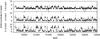 |
Fig. 1 Processed ASM lightcurve of Cen X-3 from MJD 50087 to 53501. The three energy bands A (1.5–3 keV), B (3–5 keV) and C (5–12 keV) are shown in different panels. |
The ASM instrument is an X-ray monitor covering the 1.5–12 keV energy range (Levine et al. 1996). It consists of three scanning shadow cameras (SSCs) each with a position-sensitive proportional counter (Levine et al. 1996). The counts detected in three energy bands, 1.5–3, 3–5 and 5–12 keV, are accumulated in dwells of about 90 s. In our analysis we used the dwell-by-dwell data available from the ASM team on the web1. We checked that these data differ only in format from the data available at NASA’s high energy astrophysics science archive center (HEASARC), which were used by Paul et al. (2005).
MAXI is an X-ray monitor onboard the International Space Station (ISS) (Matsuoka et al. 2009). It scans the sky in each orbit of 92 min, observing a particular source for about 40–150 s (Sugizaki et al. 2011), depending on the source position. MAXI has two cameras, the gas slit camera (GSC) and the solid-state slit camera (SSC). The main instrument, GSC, consists of proportional counters with slit and slat collimators (Matsuoka et al. 2009) with a total effective area of 5350 cm2 (Matsuoka et al. 2009). During every orbit, about 85% of the sky is scanned in the 2–30 keV energy band (Sugizaki et al. 2011). MAXI lightcurves with a time resolution of one orbit are available on the web2. The lightcurves are produced for three energy bands, 2–4 keV, 4–10 keV, and 10–20 keV.
The INTEGRAL satellite observes objects simultaneously in gamma-rays, X-rays and visible light. JEM-X is one of its instruments and consists of two telescopes with coded aperture masks (Lund et al. 2003). JEM-X obtains X-ray spectra and imaging in the 3–35 keV energy band (Lund et al. 2003). IBIS is the gamma-ray imager of INTEGRAL and consists of two detector layers, ISGRI and PICsIT (Ubertini et al. 2003). ISGRI is the soft gamma-ray imager (Lebrun et al. 2003). It consists of a CdTe detector camera with a sensitive area of 2621 cm2 observing in the 15 keV–1 MeV energy band (Lebrun et al. 2003). INTEGRAL data can be downloaded from the web3 for all instruments and for a number of predefined energy bands. For our analysis we selected the following energy bands: JEM-X 3.0–5.5 keV, 5.5–10.2 keV, 10.2–18.9 keV, 18.9–34.9 keV, ISGRI 22.1–30.0 keV, 30.0–40.3 keV, 40.3–51.2 keV, 51.3–63.3 keV.
As mentioned above, our analysis follows the procedures described in Paul et al. (2005). First, we excluded data falling in the intervals of X-ray eclipses. We then averaged the data within each orbit of the system to avoid any spectral dependence on the orbital phase (Suchy et al. 2008), i.e. we produced light curves with one time bin per orbit. For consistency, we used the same orbital parameters as Paul et al. (2005): the orbital period Porb = 2.08702 d, the mid-eclipse time tmid(TJD) = 10087.295, and the eclipse duration in units of orbital phase Δφ = 0.306 (including ingress and egress). First, we performed the analysis on the same ASM data set as used in Paul et al. (2005): from MJD 50 087 to 53 501. Then, to enlarge the data sample, we added ASM data on the source covering the time range from MJD 53 501 to 55 646 (i.e. all ASM observations available while we prepared this work). For the MAXI analysis we used all data available to date, from MJD 55 097 to MJD 55 630. For the INTEGRAL analysis we used data from MJD 52 650 to 54 959, which are all available data in the archive.
3. Results
3.1. RXTE/ASM results
The resulting ASM lightcurve of Cen X-3 in the time range MJD 50087–53501 in three energy bands with removed eclipse intervals with each bin corresponding to one orbit of the system is shown in Fig. 1. In the 5–12 keV light curve one can already see substantial differences with respect to the results of Paul et al. (2005, see Fig. 1 in their paper). We were unable to confirm the reported spectral hardening accompanied by an increase of the flux between MJD 51 800 and 53 100 in the highest energy band. The reported two spectral states should emerge as two branches of data points in a plot of the countrates in the 3–5 keV band versus the 5–12 keV band, as shown in Fig. 3 of Paul et al. (2005). In the corresponding plot from our (re-)analysis of the data (Fig. 2), we were unable to find any hint of different branches.
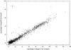 |
Fig. 2 ASM data between MJD 50 087 and 53 501 (same as used in Paul et al. 2005). Countrate in band B (3–5 keV) is plotted versus countrate in band C (5–12 keV). Typical uncertainties of the data points are indicated by the error bars in the upper left corner of the plot. |
The inclusion of the new ASM data that became available since the work of Paul et al. (2005) (MJD 53 501 to 55 646) did not reveal any separation of the data points in two spectral states either. The two modes appear neither in the new data alone, nor in the entire set of ASM data. Figure 3 shows the ASM fluxes in the 3–5 keV band versus fluxes in the 5–12 keV band. The data from the new observations (after MJD 53 501) are plotted with a different marker. We were unable to detect any change with respect to the older ASM observations.
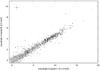 |
Fig. 3 ASM data: countrate in band B (3–5 keV) versus countrate in band C (5–12 keV). The data from MJD 50 087 to 53 501 are marked with a cross to distinguish them from the data between MJD 53 501 to 55 646, which are marked by circles. Typical uncertainties of the data points are indicated by the error bars in the upper left corner of the plot. |
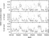 |
Fig. 4 MAXI lightcurve of Cen X-3 from MJD 55 097 to 55 630. The three energy bands 2–4 keV, 4–10 keV, and 10–20 keV are plotted. |
3.2. MAXI results
The long-term Cen X-3 lightcurve in all three energy bands of MAXI is shown in Fig. 4. We plotted the fluxes for the ASM data in different energy bands versus each other. The two spectral modes are expected to appear best in a plot of the 2–4 keV versus 4–10 keV fluxes because those energy bands are closest to the bands “B” and “C” of ASM where the clearest separation into two spectral states is seen in Paul et al. (2005). However, we were unable to find any indication of the two branches (see Fig. 5).
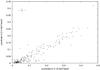 |
Fig. 5 MAXI data: countrate in the 2–4 keV band versus countrate in the 4–10 keV band. The size of typical error bars is shown in the upper left of this figure. |
3.3. INTEGRAL results
Following the procedure of Paul et al. (2005), we made countrate versus countrate plots for the selected JEM-X and ISGRI energy bands. It follows from the results of Paul et al. (2005) that the separation of the two spectral states should appear best in a 3.0–5.5 keV versus 5.5–10.2 keV countrate plot of JEM-X. As for the MAXI data, we were unable to find two spectral states (see Fig. 6). Extending the energy bands to higher energies, e.g. using ISGRI data, did not reveal any spectral separation of the source either.
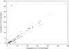 |
Fig. 6 INTEGRAL: countrate in the 3.0–5.5 keV band versus countrate in the 5.5–10.2 keV band. The size of typical error bars is shown in the upper left of this figure. |
4. Conclusions
Intrigued by the finding of Paul et al. (2005), we performed a study of Cen X-3 using the data taken with two all-sky monitors, RXTE/ASM and the MAXI as well as data taken from the JEM-X and ISGRI instruments of INTEGRAL. Using the same data and analysis procedures as Paul et al. (2005), we were unable to find any spectral transitions either in the lightcurve or by plotting fluxes in different energy bands versus each other. The result does not change with the addition of newest RXTE/ASM, MAXI or INTEGRAL data or by extending the analysis to higher energy bands. Although Paul et al. (2005) ruled out possible instrumental effects on the basis of their analysis of the ASM data of some other sources for the same time interval as for Cen X-3, we suggest that systematic and/or analysis effects are responsible for the previously reported appearance of the two spectral states. To clarify this question we contacted the ASM instrument team, inquiring whether any substantial recalibration of ASM data took place after the work of Paul et al. (2005). According to them, major calibrational changes occurred around MJD 51 956 when telemetry modes switched from ASM “position histogram” to ASM Event mode. The ASM camera SSC 1 was mainly influenced by this change and a discontinuity around that time may have led to a change in the observed fluxes as reported in Paul et al. (2005). However, the spectral discontinuity was observed in each ASM camera separately for Cen X-3, but not observed at all for a set of other pulsars. Additionally, the data software ran through major updates in April 2005 and 2007. This could also have led to the reported behavior if the data for Her X-1, Vela X-1, and SMC X-1, which were used by Paul et al. (2005) to check for possible instrumental effects, were downloaded after the software update. The instrument team also generally claimed that although it is now difficult to check whether the recalibration or data analysis software updates could have led to the reported
effect, the regular improvement of the ASM calibration over time suggests that any later analysis is generally more reliable than an earlier one.
Acknowledgments
This research has made use of the MAXI data provided by RIKEN, JAXA and the MAXI team, quick-look results provided by the ASM/RXTE team as well as data provided by the INTEGRAL Science Data Centre. We thank R. Remillard of the ASM/RXTE team for a detailed report of the history of ASM calibration and software updates. We also thank the referee for useful suggestions on improving the manuscript. This work has been partially funded by the DLR, grant 50 OR 1008, and by the Carl-Zeiss-Stiftung.
References
- Avni, Y., & Bahcall, J. N. 1974, ApJ, 192, L139 [NASA ADS] [CrossRef] [Google Scholar]
- Chodil, G., Mark, H., Rodrigues, R., et al. 1967, Phys. Rev. Lett., 19, 681 [NASA ADS] [CrossRef] [Google Scholar]
- Giacconi, R., Gursky, H., Kellogg, E., Schreier, E., & Tananbaum, H. 1971, ApJ, 167, L67 [NASA ADS] [CrossRef] [Google Scholar]
- Hutchings, J. B., Cowley, A. P., Crampton, D., van Paradijs, J., & White, N. E. 1979, ApJ, 229, 1079 [NASA ADS] [CrossRef] [Google Scholar]
- Krzeminski, W. 1974, ApJ, 192, L135 [NASA ADS] [CrossRef] [Google Scholar]
- Lebrun, F., Leray, J. P., Lavocat, P., et al. 2003, A&A, 411, L141 [NASA ADS] [CrossRef] [EDP Sciences] [Google Scholar]
- Levine, A. M., Bradt, H., Cui, W., et al. 1996, ApJ, 469, L33 [NASA ADS] [CrossRef] [Google Scholar]
- Lund, N., Budtz-Jørgensen, C., Westergaard, N. J., et al. 2003, A&A, 411, L231 [NASA ADS] [CrossRef] [EDP Sciences] [Google Scholar]
- Matsuoka, M., Kawasaki, K., Ueno, S., et al. 2009, PASJ, 61, 999 [NASA ADS] [CrossRef] [Google Scholar]
- Paul, B., Raichur, H., & Mukherjee, U. 2005, A&A, 442, L15 [NASA ADS] [CrossRef] [EDP Sciences] [Google Scholar]
- Priedhorsky, W. C., & Terrell, J. 1983, ApJ, 273, 709 [NASA ADS] [CrossRef] [Google Scholar]
- Schreier, E., Levinson, R., Gursky, H., et al. 1972, ApJ, 172, L79 [NASA ADS] [CrossRef] [Google Scholar]
- Suchy, S., Pottschmidt, K., Wilms, J., et al. 2008, ApJ, 675, 1487 [NASA ADS] [CrossRef] [Google Scholar]
- Sugizaki, M., Mihara, T., Serino, M., et al. 2011, PASJ, accepted [arXiv:1102.0891] [Google Scholar]
- Ubertini, P., Lebrun, F., Di Cocco, G., et al. 2003, A&A, 411, L131 [NASA ADS] [CrossRef] [EDP Sciences] [Google Scholar]
All Figures
|
Fig. 1 Processed ASM lightcurve of Cen X-3 from MJD 50087 to 53501. The three energy bands A (1.5–3 keV), B (3–5 keV) and C (5–12 keV) are shown in different panels. |
| In the text | |
|
Fig. 2 ASM data between MJD 50 087 and 53 501 (same as used in Paul et al. 2005). Countrate in band B (3–5 keV) is plotted versus countrate in band C (5–12 keV). Typical uncertainties of the data points are indicated by the error bars in the upper left corner of the plot. |
| In the text | |
|
Fig. 3 ASM data: countrate in band B (3–5 keV) versus countrate in band C (5–12 keV). The data from MJD 50 087 to 53 501 are marked with a cross to distinguish them from the data between MJD 53 501 to 55 646, which are marked by circles. Typical uncertainties of the data points are indicated by the error bars in the upper left corner of the plot. |
| In the text | |
|
Fig. 4 MAXI lightcurve of Cen X-3 from MJD 55 097 to 55 630. The three energy bands 2–4 keV, 4–10 keV, and 10–20 keV are plotted. |
| In the text | |
|
Fig. 5 MAXI data: countrate in the 2–4 keV band versus countrate in the 4–10 keV band. The size of typical error bars is shown in the upper left of this figure. |
| In the text | |
|
Fig. 6 INTEGRAL: countrate in the 3.0–5.5 keV band versus countrate in the 5.5–10.2 keV band. The size of typical error bars is shown in the upper left of this figure. |
| In the text | |
Current usage metrics show cumulative count of Article Views (full-text article views including HTML views, PDF and ePub downloads, according to the available data) and Abstracts Views on Vision4Press platform.
Data correspond to usage on the plateform after 2015. The current usage metrics is available 48-96 hours after online publication and is updated daily on week days.
Initial download of the metrics may take a while.