| Issue |
A&A
Volume 535, November 2011
|
|
|---|---|---|
| Article Number | A61 | |
| Number of page(s) | 8 | |
| Section | The Sun | |
| DOI | https://doi.org/10.1051/0004-6361/201117186 | |
| Published online | 04 November 2011 | |
Collisionless turbulent transport and anisotropic electron heating in coronal flare loops
Max-Planck-Institut für Sonnensystemforschung, 37191 Katlenburg-Lindau, Germany
e-mail: This email address is being protected from spambots. You need JavaScript enabled to view it.
Received: 3 May 2011
Accepted: 9 September 2011
Abstract
Context. One of the hypotheses about the generation of the hard X-ray emissions (HXR) of the sun is that a strong electron-beam is first accelerated near the looptop, and then propagated down to the chromosphere. There the HXR emissions are generated by the bombardment of electrons via thick-target bremsstrahlung. Recently, the beam-plasma model has been questioned because streaming instabilities make the beam propagation doubtful. Another open question in solar flare models is the generation of anisotropic electron distributions deduced from microwave emissions. The question is whether one can find a mechanism, in addition to the generally considered mirror motion, that may cause the electron anisotropy in flare loops.
Aims. To understand the transport of coronal electron beams and the possible generation of electron anisotropic distribution in the course of the beam propagation, we simulated a beam-plasma return-current system. Our aim is to investigate the evolution of predicted streaming instabilities at the nonlinear stage and to determine the intensity of beam transport in coronal loops.
Methods. The linear instabilities and wave coupling in the beam-plasma return-current system are investigated by a multi-fluid dispersion analysis. We performed a two-dimensional electromagnetic particle-in-cell simulation to understand the generation of turbulent transport and anisotropic electron heating at the nonlinear stage of the beam evolution.
Results. The beam-plasma return-current system is stablized at a late stage of evolution by a combined effect of 1) a relaxation of electron bulk drifts; and 2) a fast thermalization of the beam and return-current electrons in the drift direction. As a result, the downward electron beam continues to propagate in the coronal loop. Distinguishable parallel and perpendicular electron heating is observed, which is caused by turbulent deflection of electron beams. The electron distribution becomes anisotropic through different heating rates.
Conclusions. An electron beam injected from a solar flare looptop can continue to propagate stably despite a partial relaxation of its drift velocity. After drift relaxation and anisotropic electron heating, the slowed-down electron drifts and the ambient thermalized plasma create a stable beam-propagation environment because of the Landau damping effect. This electron beam can propagate stably at a modified drift speed down to the chromosphere, where it generates HXR radiation. We conclude that the beam plasma model is feasible for the HXR generation in a solar flare event. The observed anisotropic electron distribution is a direct consequence of turbulent deflections of the electron beams.
Key words: instabilities / turbulence / Sun: flares
© ESO, 2011
1. Introduction
The detailed dynamics of plasma transport in coronal flare loops has been a puzzle for many years since the electron acceleration was indirectly diagnosed by solar X-ray observations. Piece by piece, solar physicists have added different mechanisms to the picture of electron energization. Among the proposed flare scenarios a propagating electron beam in hard X-ray (HXR) coronal loops is widely considered. In the framework of the collisional thick-target model (CTTM), the footpoint HXR emission is generated by strong plasma beams ejected from the corona, causing bremsstrahlung emission in the chromosphere (De Jager 1964; Arnoldy et al. 1968; Brown 1971).
Previous solar observations from space telescopes seem to support this viewpoint. According to the standard solar flare model (Tsuneta 1997; Yokoyama & Shibata 2001), HXR observations of the synchronized looptop thermal bremsstrahlung and flare footpoint thick-target bremsstrahlung point at the coronal looptop as a primary acceleration site (Masuda et al. 1994). In this case the downward propagating beam mainly consists of accelerated electrons (Tsuneta & Naito 1998; Mann et al. 2001). Similar conclusion was drawn by model studies intended to make the picture of solar radiation in different bands coherent. For example, the closely correlated HXR emission in footpoints and radio microwave (MW) emissions in coronal loops, observed with several satellite-borne and ground-based instruments, suggest a common energy source for flare HXR radiation observed at different altitudes (Klein et al. 1986).
However, although several models of coronal acceleration seem to support the CTTM mechanism of HXR generation, several theoretical problems remain. The main difficulties are first, the so-called “number problem” – the extremely high number of electrons and beam densities needed to explain the observed intensity of the footpoint HXR radiation. And second, the maintenance of the quasi charge-neutrality in the corona, i.e. the inevitable electron resupply problem. Unfortunately, only little detailed theoretical or computational work exists on the problem of stability of return-current systems in the solar context (Fletcher 2005; Vlahos et al. 2009; Zharkova & Gordovskyy 2005). Hence, more work on instability analysis and anomalous turbulent transport is required.
Recently, taking into account the large-scale topological change of coronal magnetic fields and the resulting energy release in the form of Alfvén waves, an alternative model of turbulent acceleration directly in the chromosphere was developed to explain the observed HXR emission (Fletcher & Hudson 2008). This model attributes the generation of impulsive footpoint HXR to the energy transport via parallel Alfvén wave propagation, similar to the electron acceleration above the terrestrial aurora (Volwerk et al. 1996). Considering the typical plasma parameters of flare loops, Fletcher & Hudson (2008) concluded that Alfvén waves arrive at the chromosphere without efficient viscous or resistive damping. Hence, Alfvén waves can eventually deliver the energy for electron accelerations and HXR generation into the chromosphere. This model successfully addresses the strong intensity of footpoint HXR, without assuming a high electron beam density, as the standard CTTM model does. Note that the Alfvén wave model does not consider the electron beams in coronal loops during the flare impulsive phase.
Several observational evidence indicates, nevertheless, that electron beams in coronal loops contribute to the generation of solar HXR radiation. One of the most authentic arguments supporting the role of beams is the temporal synchronization of the looptop and footpoint HXR emissions, which indicates a common (or at least well-correlated) energy source for the radiation from the two different sites (see Fig. 2 in Masuda et al. 1994). In addition, electrons with different velocities will spend different times for the propagation in coronal loops. As a result, the time-of-flight (TOF) delay method (Aschwanden & Schwartz 1996) allows to determine fine time structures of flare HXR pulses (Aschwanden & Schwartz 1995). For most of the analyzed flare cases, with an inferred flare loop size and TOF delays measurements, the conclusion is that the particle acceleration time is much shorter than the free-streaming time. This implies that the particle acceleration takes place synchronously near the coronal looptop, but not down along the propagation path.
In order to explain the results of TOF analyses in the context of a local acceleration model, recently a so-called local re-acceleration thick-target model (LRTTM) was proposed (Brown et al. 2009). This model considers a re-acceleration mechanism caused by chromospheric turbulent waves or local current sheet electric fields, which increase the net radiative HXR output per electron injected from the HXR looptop source. The LRTTM model assumes an injection of fresh electrons from a place away from the footpoint HXR source to replace the decelerated ones (as in standard CTTM). In contrast to CTTM, however, no long-lasting high-density electron beam injection is necessary in LRTTM. Instead, the electrons are locally re-accelated to achieve the observed HXR emission (Brown et al. 2009). This model can therefore explain both the TOF delays and the long-lasting footpoint HXR emission. However, because the amount of required fresh electrons injected to chromosphere is not as high as in CTTM, there is no electron re-supply problem in LRTTM.
Hence, the electron beam propagation from a lootop source has still to be considered in solar flare models. This paper particularly aims to study the anomalous transport in beam-plasma return-current systems in coronal flare loops. The explanation of the temporal variation of the injected electron beam requires a complete reconnection/injection model in the flare looptop region (Aschwanden 1998a). However, it is beyond the scope of this paper to address the detailed electron injection from the looptop region. But a resupply return-current electron has of course to be considered. For an electron beam that propagates downward from the acceleration site in the corona, several questions have to be solved to suggest a feasible model of flare HXR emissions. One important question is the stability of the beam-plasma return-current system. It is well known that counter-streaming Maxwellian-distributed electron of comparable temperature become acoustic-wave unstable if their relative drift velocity exceeds their electron thermal velocity (Watt et al. 2002; Fletcher 2005). To understand how, nevertheless, an energetic electron beam can propagate in a coronal loop against a return-current electron beam, numerical simulations of the transport properties are necessary. An investigation including the numerical simulation of the nonlinear evolution of the return-current beam-plasma system and its anomalous transport in an unmagnetized plasma has been carried out in Lee & Büchner (2011a,b). In the following that work is considered as a reference for a comparison with the current investigation of the magnetized plasma dynamics in flare loops.
Another important question to be addressed is the origin of anisotropy of the electron distribution in coronal loops. Considering the magnetic loss-cone geometry in a flare loop, the distribution function of injected beams strongly influences the temporal evolution of HXR emissions at the footpoint (Aschwanden 1998b). A theoretical investigation of the electron thermalization in a beam-plasma return-current system was carried out by using a three-dimensional particle-in-cell simulation (3D PIC) by Karlický & Bárta (2009). The authors concluded that in weak magnetic fields a filamentation instability strongly heats the electrons perpendicular to the direction of beam propagation. In unmagnetized plasmas, turbulent field perturbations cause a deflection of the pre-heated parallel electron flows, which results in distinct parallel and perpendicular heating rates (Lee & Büchner 2011a,b). These previous investigations demonstrate that the evolution of the electron distribution from isotropic to anisotropic can be a result of several kinds of instabilities. The evolution of electron distribution functions from the looptop acceleration sites to the chromospheric HXR sites is important for understanding the transport process in solar flare loops. In principle, the anisotropy of precipitating particles can be detected by polarimetric observations in flares located between the solar center and the limb (Suarez-Garcia et al. 2006; Boggs et al. 2006). So far, most models of the electron transport during solar flares considered that anisotropy is primarily generated by a magnetic mirror mechanism. Numerical investigations of the beam electron kinetics of precipitating electron beams were carried out, e.g., by Zharkova et al. (Zharkova & Gordovskyy 2005). These authors concluded that the anisotropic electron distribution plays an important role in the observed HXR and MW emissions and should be included in models of the solar flare dynamics (Zharkova et al. 2010a,b). The question arises, however, whether there is another mechanism that generates anisotropic distribution in flare loops, in addition to the usually assumed magnetic mirror mechanism.
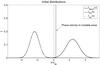 |
Fig. 1 Distributions of the beam-plasma return-current system considered for solar flare loops. The expected phase velocity of an initially unstable wave is plotted as a black dashed line. |
In this paper, a beam-plasma return-current system is considered to study the two mentioned important questions in solar flare radiation, i.e. the stability evolution of a return-current system, and the generation of anisotropic electron distributions. The two-dimensional, relativistic, and electromagnetic particle-in-cell (PIC) code XOOPIC (Verboncoeur et al. 1995) was used for this study. But we first carry out a multifluid dispersion analysis in Sect. 2 to study the linear electromagnetic stability properties of the beam-plasma return-current system for typical parameters of the flare coronal plasma. In Sect. 3 simulation results of the nonlinear evolution of wave-particle interaction and of the consequent anomalous transport are provided and a spectrum analysis of the field perturbations is given. We compare the temporal evolution of the turbulence and of the energy conversion between kinetic and thermal energy in Sect. 4. We find anisotropic electron heating at the nonlinear stage of the beam evolution, and we discuss its correlation with the growth of localized turbulences. In the conclusion we discuss the possible implication for energetic electron beam propagation in the solar flare loops.
2. Model setup and multifluid dispersion analysis
To study the anomalous transport and stability of electrons in a coronal flare loop, a two-dimensional beam-plasma return-current configuration is considered for the linear dispersion analysis and for the particle-in-cell simulation. A sketch is shown in Fig. 1. A charge- and current-neutrality system is assumed, i.e.  (1)where Nα is the density and Vdα is the bulk velocity of the plasma species α. The same plasma configuration was used e.g. in the papers of Lee & Büchner (2011a,b) for the investigation of the plasma evolution in an environment without background magnetic fields. In this work, we assume a background magnetic field Bx = 100 G to mimic the magnetized coronal loops. In an solar active region this value is typical for the loop magnetic field during flares (Masuda et al. 1994), and the value is usually deduced from the gyro-synchrotron radiation of micro-wave observations (Kundu et al. 2001).
We use the typical plasma parameters inferred for coronal flare loops throughout: 1) number density of background ions ni = 1 × 10¹⁶ m-3 and of two drifting electron beams ne,beam = ne,RC = 5 × 10¹⁵ m-3; 2) temperature of hot-forward propagating electron beam Te,beam = 2Tion = 2Te,RC, which is twice of the background ions and return-current electrons. The temperature of the injected electron beam is Te,beam = 2 keV, which corresponds to an electron thermal velocity Vte ≈ 0.088 c; 3) the drifts of beam and return-current electrons are directed opposite to each other (Vde,beam = −Vde,RC), leaving the net current zero. The real ion-to-electron mass ratio is applied (mi/me = 1836). The drift velocity is choosen 2.4 times of the electron thermal velocity (Vde = 2.4Vte), referring to a fast injected electron beam from the looptop. The same parameters as for plasma setup are used for the dispersion analysis and, again, in the later 2D EM PIC code simulation to investigate the nonlinear evolution. Note that the subscripts “beam” ”and “RC” here represent the beam and return-current electrons. In the simulation they are equivalent to the electron species “e1” and “e2”.
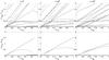 |
Fig. 2 Linear dispersion for propagation angles θ = 0°;θ = 30°;θ = 60°. Dotted lines depict the normalized real frequencies ω(k) of waves, crosses depict the corresponding growth rates γ(k). |
In the considered beam-plasma return-current system, drifting Maxwellian electron distribution functions become unstable with the free energy supply from the drifts. At the linear stage of plasma evolution the system can be investigated in the fluid regime because the drifts of electrons are well above the electron- and ion-thermal velocities. Hence, Landau damping (Landau 1946) is initially negligible. Therefore, for the stability analysis a multi-fluid dispersion relation, i.e. Eq. (2.20) in Lee (2008) or Eq. (8) in Lee & Büchner (2011b), can be used for the investigation of eigen modes and instabilities. We calculated the multi-fluid dispersion relation with the applied plasma parameters. The resulting waves and instabilities are shown in Fig. 2 for propagation angles θ = 0°;θ = 30°;θ = 60°.
The dispersion relation is considered only for two electron species in the rest frame of the return-current electrons. Background ions can be neglected because the real electron-ion mass ratio is applied in this study. The reason for the simplification is that theoretically and numerically it has been proved that the anomalous transport in the beam-plasma return-current system is mainly caused by interactions between electrons (Lee et al. 2008). The wave coupling in a multi-species system can be studied by considering the interaction of only two species each time if the characteristics (phase velocities) of the other wave modes are far from the coupling region. In the considered beam-plasma return-current system, wave coupling between electron- and ion- related waves exists indeed. The corresponding instabilities growth rate is, however, negligible compared to the growth rate caused by wave coupling of the two electron species (Lee et al. 2007). As one can see in Fig. 2, numerous eigen modes exist in the system. The streaming instabilities, as indicated by their positive growth rates (crosses in Fig. 2), are caused by the energy exchange between waves of positive and negative energy (Chen 1987).
The upper column of Fig. 2 shows the complete dispersion curves at different angles. These dispersion diagrams help to identify the original unstable modes. In the lower column, on the other hand, the unstable branches in the upper are dipicted with their corresponding growth rates. We found that the highest growth rate is caused by the coupling between 1) backward propagating electron acoustic waves (in the − x direction) of the return-current electron beam; and 2) the forward propagating electron acoustic wave (to the + x direction) of the hot beam of precipitating electrons. The electron-electron acoustic instability is electrostatic in nature. In addition to the primary instability caused by coupling of two electron acoustic waves, other unstable waves can be excited at oblique propagation angles. The oblique modes are caused by coupling to electron cyclotron waves. In general, they have much smaller growth rates compared to the primary electron-electron acoustic mode. Because these waves are triggered by cyclotron waves, they generate magnetic field perturbations.
The multi-fluid dispersion analysis used here is reliable only for wavelengths longer than the Debye length, i.e. the minimum wave length covered by a fluid description is kλde < 1. If kinetic effects are included, waves and instabilities in the range kλde ≥ 1 beome Landau-damped. The predicted waves and instabilities only describe the linear phase of instabilities. Soon the system leaves the linear stage and evolves into a non-linear state. To understand the anomalous transport, it is important to know how the linear instabilities develop into field perturbations and flow turbulences at the nonlinear stage.
In the following sections, the nonlinear evolution of the system is studied by means of a two-dimensional electromagnetic particle-in-cell simulation (2DEM PIC).
3. Collisionless momentum transport by electromagnetic turbulences
Owing to the linearly predicted streaming instabilities in a beam-plasma return-current system, one of the controversies is about the propagation of such electron beam in flare loops (Fletcher 2005). The primary argument is whether the anomalous transport, generated by the instabilities, would dissipate the injected electron beam significantly so that it is unable ever to make its way to the chromosphere. In the view of plasma transport one has to answer the following question: given typical flare plasma parameters, under which condition can an injected plasma beam eventually propogate down to the chromosphere stably and hence generate HXR?
To investigate the nonlinear evolution of the injected electron beam, we used the two-dimensional electromagnetic particle-in-cell code XOOPIC (Verboncoeur et al. 1995). To include the wave-particle resonance effect at kinetic scales the implemented grid size was chosen to be smaller than the Debye length (dx = dy = λDe/4). The simulation domain is Lx = 512λde and Ly = 128λde. Periodic boundary condition was applied in both directions. The simulation box is more than an order of magnitude larger than the typical wave length of the expected main turbulence mode generated by electron/ion acoustic type instabilities (Lee et al. 2008), and of the coupled cyclotron instabilities.
The simulation was performed sufficiently long for the relaxation of electron drifts and the anisotropic heating to be saturated. The energy of the resulting electromagnetic field perturbation is plotted in Fig. 3, starting from the linear and continuing down to the nonlinear stage of instability development ( ). The generated electric field and magnetic field energy in the whole simulation domain are shown as a function of time in Fig. 4. The upper panel of Fig. 3 shows that the wave fronts of the perturbations propagate obliquely, approximately in the range ( − 30° ≤ θ ≤ 30°), where θ is the angle between k and background magnetic field Bx.
The result of a spectrum analysis of the generated electric and magnetic field perturbations is shown in Fig. 5. The left panels of this figure depict the spectra of electric and magnetic field perturbations during the linear stage ![Mathematical equation: \hbox{$t\subset[0; 38.25]\omega_{\rm pe}^{-1}$}](/articles/aa/full_html/2011/11/aa17186-11/aa17186-11-eq30.png) . The right panels show the wave spectra at the nonlinear evolution stage
. The right panels show the wave spectra at the nonlinear evolution stage ![Mathematical equation: \hbox{$t\subset[38.25; 765]\omega_{\rm pe}^{-1}$}](/articles/aa/full_html/2011/11/aa17186-11/aa17186-11-eq31.png) . The frequencies of the spectrum shown in the figure are chosen following the highest intensities in the frequency range. At other frequencies we found a much lower spectral intensity. In the linear stage (left panels), the perturbations have typical wavelengths longer than Debye length (k||λDe ≤ 1; k⊥λDe ≤ 1), as expected from the linear dispersion analysis (see Fig. 2). Shorter wavelength perturbations (k||λDe ≥ 1; k⊥λDe ≥ 1) experience Landau damping, therefore they do not exist. Comparing the spectrum of electric and magnetic perturbations, we found that (the left lower panel) magnetic perturbations propagate more in the oblique direction, as can be seen by the wider extension in the k ⊥ coordinate. The electric perpurbations propagate at a smaller angle, more parallel to the background magnetic field. At the nonlinear stage large amplitude waves grow by merging smaller wave perturbations.
. The frequencies of the spectrum shown in the figure are chosen following the highest intensities in the frequency range. At other frequencies we found a much lower spectral intensity. In the linear stage (left panels), the perturbations have typical wavelengths longer than Debye length (k||λDe ≤ 1; k⊥λDe ≤ 1), as expected from the linear dispersion analysis (see Fig. 2). Shorter wavelength perturbations (k||λDe ≥ 1; k⊥λDe ≥ 1) experience Landau damping, therefore they do not exist. Comparing the spectrum of electric and magnetic perturbations, we found that (the left lower panel) magnetic perturbations propagate more in the oblique direction, as can be seen by the wider extension in the k ⊥ coordinate. The electric perpurbations propagate at a smaller angle, more parallel to the background magnetic field. At the nonlinear stage large amplitude waves grow by merging smaller wave perturbations.
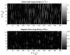 |
Fig. 3 Spatial distributions of electric field and magnetic field energy density in the simulation domain at time |
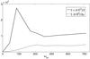 |
Fig. 4 Generated electric field (solid line) and magnetic field (dashed line) energy as function of time. |
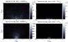 |
Fig. 5 Spectrum analysis of simulation in the linear stage (left panels) and nonlinear stage (right panels). The analyzed interval for the linear stage is |
At the nonlinear stage the frequency of the dominant mode is much lower than the frequency of the maximum growing mode at the linear stage. The phase velocity at the nonlinear stage is also much lower than the phase velocity of the most unstable mode at the linear stage. The wavelength of the most intensive nonlinear wave perturbations is longer in the short wave number range. This can be seen in the right panels for both electric and magnetic perturbations. Similar shifts were found also in electrostatic perturbation in previous investigations of one-dimensional electrostatic instabilities (Lee et al. 2008). In addition to the wavelength shifts at the nonlinear stage, the electric perturbations are propagating more parallel than in the linear stage. Furthermore, at the nonlinear stage the amplitude of the electric perturbation exceeds the amplitude of magnetic perturbation by about an order of magnitude. This simulation result corresponds well to the dispersion analysis, i.e. the electromagnetic cyclotron instability has a much lower growth rate than the electron acoustic instability.
At the nonlinear stage of the field perturbation growth, the electron beam and return current are slowed. The growth of streaming instabilities first converts the kinetic energy of the electron beams into electromagnetic field energy, and later the wave energy is further converted into electron thermal energy. The temporal evolution of electron beam and return-current drifts is shown in the left panel of Fig. 6.
Together with drift relaxation, anisotropic electron heating also takes place. Parallel and perpendicular electron temperatures are shown in the middle and right panels of Fig. 6. Evidently the original isotropic (Tx,e1 = Ty,e1; Tx,e2 = Ty,e2 at t = 0) beam and return-current electrons are thermalized at different rates. The parallel electron thermalization saturates at  , which is the same instant that the intense drift relaxation finishes. The parallel electron temperature reaches the level Tx,e1 = 6.24 keV and Tx,e2 = 4.99 keV at a later stage of simulation. The perpendicular electron temperature, on the other hand, continues to increase until a much later time
  , and the final perpendicular electron temperatures becomes Ty,e1 = 3.12 keV and Ty,e2 = 2.18 keV. Hence, in the course of beam propagation the original isotropic drifting Maxwellian distributions of electron beams evolve into anisotropic ones. Anisotropic electron heating has already been reported in Lee & Büchner (2011b), who considered the case without a background magnetic field Bx. By comparing the simulation results, one notices that the perpendicular electron heatings are stronger in the unmagnetized case (Lee & Büchner 2011b), which are Ty,e1 = 4.99 keV and Ty,e2 = 3.74 keV at the end of simulation.
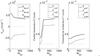 |
Fig. 6 Temporal evolution of the bulk drifts of beam electron (solid line) and return-current electron (dashed line), plasma heating in the parallel and in the perpendicular directions. |
Clearly the kinetic energy of the electron beams is first converted into the energy of electromagnetic turbulences. At the later stage the field energy is then transformed into electron thermal energy. However, the energy conversion mechanism in magnetized plasma is different from the one in unmagnetized plasma. In an unmagnetized plasma without background magnetic field the perpendicular electron heating is caused by turbulent deflection of the parallel flow (Lee & Büchner 2011a,b). The turbulent deflection has a tendency to reduce the temperature anisotropy. On the other hand, in a magnetized plasma with a strong background magnetic field, as in coronal loops, the plasma turbulent deflection can be suppressed by the magnetic field tension force.
The applied background magnetic field changes the processes of energy conversion as well as the anisotropic electron heating. We will discuss how the magnetic tension influences the energy conversion and the associated perpendicular electron motion in the next section.
4. Energy conversion and electron heating
Anisotropic electron heating caused by electron turbulent deflections in an unmagnetized plasma has been discussed in Lee & Büchner (2011b). For the anisotropic electron heating in magnetized plasma we examined the localized turbulence and the intensity of electron perpendicular flow. Initially, the beam and return-current electrons are flowing in parallel to the magnetic field background Bx. At the nonlinear stage  , the beam and return-current drifts are deflected, and the electron flows pick up perpendicular velocity. The flow patterns are plotted in the upper and lower panels of Fig. 7. To demonstrate this effect, we show the amount of the electron drift deflection described by the averaged perpendicular momentum in Fig. 8. Obviously, the perpendicular momentum increases synchronously with the relaxation of electron bulk drifts (
 cf. the first panel of Fig. 6). This indicates that the parallel momentum of electron beams, drifting initially in the x direction, is re-directed to the perpendicular y direction.
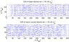 |
Fig. 7 Flow velocity arrows of the beam (upper) and return-current (lower) electrons. |
However, Fig. 8 also indicates that the perpendicular momentum does not further increase during the nonlinear stage (after  ), although the parallel momentum (drift) is still dropping slowly (cf. Fig. 6). Because the energy is conserved in the system, this indicates a loss of the kinetic energy of the parallel drift motion and its conversion to other energy forms. One immediately notices that the perpendicular electron heating (shown in the third panel of Fig. 6) continues even after the primary drift relaxation stops at . The continued perpendicular electron heating indicates that the perpendicular thermalization mechanism is different from the one of parallel electron heating, where the later one is mainly caused by the interaction with parallel electric field fluctuations (Büchner & Elkina 2005; Lee et al. 2008; Lee & Büchner 2010).
As discussed in the previous section, at the early nonlinear stage the parallel electron heating is faster than the perpendicular electron heating. To confirm that the long-lasting perpendicular electron heating is supplied by the deflected thermal energy, the heat flux diverted from parallel to perpendicular direction should be calculated. The heat flux caused by the parallel-to-perpendicular deflection can be estimated as follows  (2)A detailed derivation of the diverted heat flux (Eq. (2)) can be found in Lee & Büchner (2011b). In the above equation the term Tα, | | − Tα, ⊥ is the temperature difference between parallel and perpendicular directions. Clearly, according to Eq. (2) the deflected heat flux Qy vanishes if there is no temperature difference, i.e. (Tα, | | − Tα, ⊥ = 0).
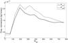 |
Fig. 8 Averaged perpendicular momentum of electrons (solid line = beam electron, dashed line = return current), shown as functions of time. |
In the right panel of Fig. 10 the estimated perpendicular heat flux (Qy), which is deflected from the parallel to the perpendicular flow direction is plotted as a function of time. The perpendicular heating rate ∂Ty/∂t is plotted in the left panel as a reference for the increase of the perpendicular thermal energy. These two panels show a synchronic evolution of perpendicular heating rate and deflection of heated parallel electron flow to the perpendicular direction. This indicates that the diverted parallel electron flows, pre-heated in the parallel direction, turn in the perpendicular direction by turbulent scattering and carry their thermal energy along. The turbulent deflection of the electron flows, as shown in Fig. 7, explains the continued perpendicular electron heating after the parallel electron heating has saturated at .
As pointed out in the previous section, evidently, a stronger anisotropy of the electron distribution is generated because of the existence of the background magnetic field Bx. We suspect that the magnetic tension force is the cause of this strong anisotropy. This hypothesis will be tested here by a detailed analysis of the forces applied to the plasma.
In general, the deflection of pre-heated parallel electron drifts is caused by the out-of-plan magnetic perturbation δBz. This is the mechanism that generates the perpendicular heating in both magnetized and unmagnetized plasma. However, when a background Bx appears, the Lorentz force can regulate the plasma motion. The Lorentz force of FLorentz = J × B has two parts  (3)where the first term on the right-hand side is the gradient of magnetic pressure, and the second term is the magnetic tension force. If the field lines are not straight but have a radius of curvature R, a transverse tension force B2/(μ0R) is exerted per unit volume (Harra & Mason 2004).
For an imposed background magnetic field Bx = 100 G, the background magnetic field applies magnetic tension force when the field topology has a curvature. The background magnetic field in a magnetized collisionless plasma is bent with the perpendicular electron flows. Consequently, the magnetic tension force of the background magnetic field acts as a restoring force and suppresses the perpendicular electron drifts. Indeed the highest averaged perpendicular momentum in this magnetized plasma case is only | Py,e1,e2 | mag. ≈ 0.8 | Py,e1,e2 | unmag., compared to the maximum perpendicular momentum of unmagnetized plasma (see Fig. 7 in Lee & Büchner 2011b).
The magnetic tension force (B· ▽ )B/μ0 as a function of time is calculated for the magnetized and unmagnetized cases and they are shown in Fig. 9. Because of the applied background magnetic field, Bx = 100 G is much larger than the generated magnetic field turbulences (at the nonlinear stage the out-of-plan magnetic perturbation δBz is smaller in the magnetized plasma δBz ≈ 5 − 15 G, than in the unmagnetized case (where δBz ≈ 10 − 20 G, Lee & Büchner 2011b). The generated magnetic tension force, which suppresses the perpendicular electron flow, is much stronger in magnetized plasma (circled solid line in Fig. 9) than the generated tension force in unmagnetized plasma (solid line in Fig. 9). The stronger magnetic tension force explains the suppressed perpendicular momentum in this case.
A direct consequence of the suppressed perpendicular flow is that the perpendicular heat flux Qy is also much reduced, as expressed in Eq. (2). With a reduced perpendicular heat flux in the case of magnetized plasma, the perpendicular electron heating rate is also weaker. A stronger anisotropy is caused by the less efficient perpendicular heating when the background magnetic field is imposed. As shown in Fig. 6, the temperature anisotropies of beam and return-current electrons are Tx,e1/Ty,e1 = 2 and Tx,e2/Ty,e2 = 2.29 at the final stage of evolution in this case, while for the same simulation setup but without background magnetic field the reported electron temperature anisotropies were Tx,e1/Ty,e1 = 1.27 and Tx,e2/Ty,e2 = 1.33 (Lee & Büchner 2011b).
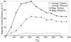 |
Fig. 9 Grid-averaged tension force (solid lines) and magnetic pressure gradient (dashed lines) for magnetized (with circle marks) and unmagnetized plasma. |
It is shown here, therefore, that the anisotropic heating of both beam and return current electrons is more prominent in the presence of a finite background magnetic field. The result suggests that the anisotropic electron distribution is a natural consequence of beam propagation that undergoes turbulent transport in waves generated by initially fluid-like instabilities.
It is worthwhile to address the evolution of electron drifts. As Fig. 6 shows, the strong relaxation of electron drifts, which has been argued to be a result of turbulent transport, comes to an end when the parallel electron heating saturates. It has been proven in multi-fluid and kinetic regimes (Lee & Büchner 2010) that the beam-plasma return-current system evolves into a stable state at the late stage of the nonlinear evolution with slow drifts and high electron temperatures, because of a strong Landau damping effect. It is demonstrated again here that in the beam-plasma return-current system the instabilities cease after the thermalization of drifting electrons, if there is either a background magnetic field or no external B-field.
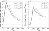 |
Fig. 10 Perpendicular heating rate ∂Ty/∂t (left panel) and heat flux Qy deflected from parallel to perpendicular direction (right panel). The solid, dashed and dotted lines are calculated values of beam electron, return-current electron and background ion, respectively. |
5. Discussion and conclusion
We studied the turbulent transport in a beam-plasma return-current system for typical solar plasma conditions inferred from flare observations. This work was carried out by means of a linear stability analysis and a two-dimensional electromagnetic particle-in-cell simulation.
We found that in the course of nonlinear evolution the beam electron drift relaxes and anisotropic electron heating takes place. The initial beam plasma situation is unstable, several linear instabilities are indentified by a multi-fluid dispersion analysis. Once the instabilities develop into a nonlinear stage, the electron beam drifts are slowed down and the electrons are anisotropically thermalized. As a result of the reduced drift velocities, Landau damping comes into play. This stabilizes waves with wavelengths shorter than the Debye length (Lee & Büchner 2010).
The whole beam evolution proceeds in the following way: 1) the original beam-plasma return-current system is unstable against the excitation of electron acoustic and electron cyclotron waves. These waves with wavelengths longer than the Debye length can be adequately described by a multi-fluid approach; 2) the linear fluid instabilities nonlinearly trigger unstable waves. Their amplification causes a large-scale magnetic field turbulence δBz, deflecting electron flows and causing turbulent transport. Anisotropic electron heating takes place as a result of continuous electron drift deflection by the magnetic turbulence; 3) along with the slowdown of electron drifts, Landau damping starts. The most unstable waves, predicted in the multi-fluid dispersion analysis, are now in the short wavelength range. The kinetic wave-particle interaction comes into play, therefore the instabilities are Landau-damped (Landau 1946). As a result, the waves cannot grow to larger amplitudes and the slowed electron beams can continue to propagate downward to the chromosphere, where they excite HXR radiations.
This kinetic investigation of the beam-plasma return-current system explains how the energetic electron beam injected from the looptop region can heat the plasma in coronal loops to a certain degree while propagating to the site of HXR emission in the chromosphere. It also addresses the anisotropic electron distribution as a natural consequence of the beam propagation. Anisotropic distribution can be generated directly by the propagating beam, in addition to the generally assumed magnetic mirror motion. This effect was recently found already in the return-current beam plasma system without background magnetic field (Lee & Büchner 2011a,b).
To compare with our previous investigations of the beam transport in coronal loops, we point out that the perpendicular electron heating was studied in different background magnetic fields by means of 3D particle-in-cell simulation (Karlický & Bárta 2009). Without the analysis of turbulent transport and magnetic tension force effect, these authors found that the perpendicular electron heating is reduced in stronger background B-fields. Now it is clear that the anisotropic electron heating is caused by the perpendicular heat flux, which is the result from drift deflection of pre-heated parallel electron beam.
Acknowledgments
The authors are grateful to the Max-Planck Society for funding this work by the Interinstitutional Research Initiative “Turbulent transport and ion heating, reconnection and electron acceleration in solar and fusion plasmas” Project No. MIF-IF-A-AERO8047.
References
- Arnoldy, R. L., Kane, S. R., & Winckler, J. R. 1968, ApJ, 151, 711 [NASA ADS] [CrossRef] [Google Scholar]
- Aschwanden, M. J. 1998a, ApJ, 502, 455 [NASA ADS] [CrossRef] [Google Scholar]
- Aschwanden, M. J. 1998b, in Observational Plasma Astrophysics: Five Years of YOHKOH and Beyond, ed. T. Watanabe et al., Astrophys. Space Sci. Lib. (Boston, Mass.: Kluwer Academic Publishers), 229, 285 [Google Scholar]
- Aschwanden, M. J., & Schwartz, R. A. 1995, ApJ, 455, 699 [NASA ADS] [CrossRef] [Google Scholar]
- Aschwanden, M. J., & Schwartz, R. A. 1996, ApJ, 464, 974 [NASA ADS] [CrossRef] [Google Scholar]
- Boggs, S. E., Coburn, W., & Kalemci, E. 2006, ApJ, 638, 1129 [NASA ADS] [CrossRef] [Google Scholar]
- Brown, J. C. 1971, Sol. Phys., 18, 489 [NASA ADS] [CrossRef] [Google Scholar]
- Brown, J. C., Turkmani, R., Kontar, E. P., MacKinnon, A. L., & Vlahos, L. 2009, A&A, 508, 993 [NASA ADS] [CrossRef] [EDP Sciences] [Google Scholar]
- Büchner, J., & Elkina, N. 2005, Space Sci. Rev., 121, 237 [NASA ADS] [CrossRef] [Google Scholar]
- Chen, L. 1987, Waves and instabilities in plasmas, World Scientific Lecture Notes in Physics (NJ: World Scientific Publishing Co. Pte. Ltd.), 12, 20 [Google Scholar]
- De Jager, C. 1964, Solar X-radiation, in Astronomical Observations From Space Vehicles, ed. J.-L. Steinberg (Lieǵe, Belgium: Taffin-Lefort), 45 [Google Scholar]
- Fletcher, L. 2005, Space Sci. Rev., 121, 141 [NASA ADS] [CrossRef] [Google Scholar]
- Fletcher, L., & Hudson, H. S. 2008, ApJ, 675, 1645 [NASA ADS] [CrossRef] [Google Scholar]
- Harra, L. K., & Mason, Keith, O. 2004, Space Sci. (London: Imperial College Press) [Google Scholar]
- Karlický, M., & Bárta, M. 2009, Nonlin. Processes Geophys., 16, 525 [Google Scholar]
- Klein, K.-L., Trottet, G., & Magun, A. 1994, SoPh, 104, 243 [NASA ADS] [Google Scholar]
- Kundu, M. R., Grechnev, V. V., Garaimov, V. I., & White, S. M. 2001, ApJ, 563, 389 [NASA ADS] [CrossRef] [Google Scholar]
- Kuznetsov, A. A., & Zharkova, V. V. 2010, ApJ, 722, 1577 [NASA ADS] [CrossRef] [Google Scholar]
- Landau, L. D. 1946, J. Phys. (USSR), 10, 25 [Google Scholar]
- Lee, K. W. 2008, Collisionless Transport of Energetic Electrons in the Solar Corona, Ph.D. Thesis, Graduate Institute of Space Science, National Central University, Taiwan [Google Scholar]
- Lee, K. W., & Büchner, J. 2010, Phys. Plasmas, 17, 042308 [NASA ADS] [CrossRef] [Google Scholar]
- Lee, K. W., & Büchner, J. 2011a, Advances in Plasma Astrophysics, Proc. IAU Symp., 274, 102 [NASA ADS] [Google Scholar]
- Lee, K. W., & Büchner, J. 2011b, Phys. Plasmas, 18, 022308 [NASA ADS] [CrossRef] [Google Scholar]
- Lee, K. W., Büchner, J., & Elkina, N. 2007, Phys. Plasmas, 14, 112903 [NASA ADS] [CrossRef] [Google Scholar]
- Lee, K. W., Büchner, J., & Elkina, N. 2008, A&A, 478, 889 [NASA ADS] [CrossRef] [EDP Sciences] [Google Scholar]
- Mann, G., Clasen, H.-T., & Motschmann, U. 2001, JGR, 106, 25323 [Google Scholar]
- Masuda, S., Kosugi, T., Hara, H., Tsuneta, S., & Ogawara, Y. 1994, Nature, 371, 495 [NASA ADS] [CrossRef] [Google Scholar]
- Suarez-Garcia, E., Hajdas, W., Wigger, C., et al. 2006, Sol. Phys., 239, 149 [NASA ADS] [CrossRef] [Google Scholar]
- Tsuneta, S. 1997, ApJ, 483, 507 [NASA ADS] [CrossRef] [Google Scholar]
- Tsuneta, S., & Naito, T. 1998, ApJ, 495, L67 [NASA ADS] [CrossRef] [Google Scholar]
- Verboncoeur, J. P., Langdon, A. B., & Gadd, N. T. 1995, Comput. Phys. Commun., 87, 199 [NASA ADS] [CrossRef] [Google Scholar]
- Vlahos, L., Krucker, S., & Cargill, P. 2009, Lect. Not. Phys., 778, 157 [NASA ADS] [CrossRef] [Google Scholar]
- Volwerk, M., Louarn, P., Chust, T., Roux, A., & de Feraudy, H. 1996, J. Geophys. Res., 101, 13, 335 [CrossRef] [Google Scholar]
- Watt, C. E., Horne, R. B., & Freeman, M. P. 2002, Geophys. Res. Lett., 29, 1004 [NASA ADS] [CrossRef] [Google Scholar]
- Yokoyama, T., & Shibata, K. 2001, ApJ, 549, 1160 [NASA ADS] [CrossRef] [Google Scholar]
- Zharkova, V. V., & Gordovskyy, M. 2005, A&A, 432, 1033 [NASA ADS] [CrossRef] [EDP Sciences] [Google Scholar]
- Zharkova, V. V., Kuznetsov, A. A., & Siversky, T. V. 2010, A&A, 512, A8 [NASA ADS] [CrossRef] [EDP Sciences] [Google Scholar]
All Figures
|
Fig. 1 Distributions of the beam-plasma return-current system considered for solar flare loops. The expected phase velocity of an initially unstable wave is plotted as a black dashed line. |
| In the text | |
|
Fig. 2 Linear dispersion for propagation angles θ = 0°;θ = 30°;θ = 60°. Dotted lines depict the normalized real frequencies ω(k) of waves, crosses depict the corresponding growth rates γ(k). |
| In the text | |
|
Fig. 3 Spatial distributions of electric field and magnetic field energy density in the simulation domain at time |
| In the text | |
|
Fig. 4 Generated electric field (solid line) and magnetic field (dashed line) energy as function of time. |
| In the text | |
|
Fig. 5 Spectrum analysis of simulation in the linear stage (left panels) and nonlinear stage (right panels). The analyzed interval for the linear stage is |
| In the text | |
|
Fig. 6 Temporal evolution of the bulk drifts of beam electron (solid line) and return-current electron (dashed line), plasma heating in the parallel and in the perpendicular directions. |
| In the text | |
|
Fig. 7 Flow velocity arrows of the beam (upper) and return-current (lower) electrons. |
| In the text | |
|
Fig. 8 Averaged perpendicular momentum of electrons (solid line = beam electron, dashed line = return current), shown as functions of time. |
| In the text | |
|
Fig. 9 Grid-averaged tension force (solid lines) and magnetic pressure gradient (dashed lines) for magnetized (with circle marks) and unmagnetized plasma. |
| In the text | |
|
Fig. 10 Perpendicular heating rate ∂Ty/∂t (left panel) and heat flux Qy deflected from parallel to perpendicular direction (right panel). The solid, dashed and dotted lines are calculated values of beam electron, return-current electron and background ion, respectively. |
| In the text | |
Current usage metrics show cumulative count of Article Views (full-text article views including HTML views, PDF and ePub downloads, according to the available data) and Abstracts Views on Vision4Press platform.
Data correspond to usage on the plateform after 2015. The current usage metrics is available 48-96 hours after online publication and is updated daily on week days.
Initial download of the metrics may take a while.