| Issue |
A&A
Volume 535, November 2011
|
|
|---|---|---|
| Article Number | A118 | |
| Number of page(s) | 14 | |
| Section | Galactic structure, stellar clusters and populations | |
| DOI | https://doi.org/10.1051/0004-6361/201116957 | |
| Published online | 22 November 2011 | |
Planetary nebulae as observational constraints in chemical evolution models for NGC 6822
1
Instituto de Astronomía, Universidad Nacional Autónoma de México, Apdo. Postal 70264, Méx. DF, 04510 México, Mexico
e-mail: This email address is being protected from spambots. You need JavaScript enabled to view it.
; This email address is being protected from spambots. You need JavaScript enabled to view it.
; This email address is being protected from spambots. You need JavaScript enabled to view it.
2
Instituto Nacional de Astrofísica, Optica y Electrónica, Luis Enrique Erro No. 1, Puebla, Mexico
e-mail: This email address is being protected from spambots. You need JavaScript enabled to view it.
Received: 24 March 2011
Accepted: 30 August 2011
Abstract
Aims. Chemical evolution models are useful for understanding the formation and evolution of stars and galaxies. Model predictions will be more robust when more observational constraints are used. We present chemical evolution models for the dwarf irregular galaxy NGC 6822 using chemical abundances of old and young planetary nebulae (PNe) and H ii regions as observational constraints. We use two sets of chemical abundances, one derived from collisionally excited lines (CELs) and one from recombination lines (RLs). We use our models as a tool to distinguish between both procedures for abundance determinations.
Methods. In our chemical evolution code the chemical contribution of low and intermediate mass stars is time-delayed, while for the massive stars the chemical contribution follows the instantaneous recycling approximation. Our models have two main free parameters: the mass-loss rate of a well-mixed outflow and the upper mass limit, Mup, of the initial mass function (IMF). To reproduce the gaseous mass and the present-day O/H value we need to vary the outflow rate and the Mup value.
Results. We calculate two models with different Mup values that reproduce the constraints adequately. The abundances of old PNe agree with our models and support the star-formation history derived independently from photometric data. Both require an early well-mixed wind, lasting 5.3 Gyr, to reproduce the observed gaseous mass in the galaxy. In addition, by assuming a fraction of binaries producing SNIa of 1%, the models fit the Fe/H abundance ratio as derived from A supergiants. The first model (M4C), which assumes Mup = 40 M⊙, fits within errors smaller than 2σ the O/H, Ne/H, S/H, Ar/H and Cl/H abundances obtained from CELs for old and young PNe and H ii regions. The second model (M1R), which adopts Mup = 80 M⊙, reproduces within 2σ errors the O/H, C/H, Ne/H and S/H abundances adopted from RLs. Both models reproduce the increase of the O, Ne, S, and Ar elements during the last 6 Gyr. We are not able to match the observed N/O ratios in either case, which suggests that the N yields of LIMS need to be improved. Model M1R does not provide a good fit to the Cl/H and Ar/H ratios, because the SN yields of those elements for m > 40 M⊙ are not adequate and need to be improved (two sets of yields were tried). From these results we are unable to conclude which set of abundances (the one from CELs or the one from RLS) represents the real abundances in the ISM better. We discuss the predicted ΔY/ΔO values, finding that the value from model M1R agrees better with data for other galaxies from the literature than the value from model M4C.
Key words: ISM: abundances / galaxies: evolution / galaxies: dwarf / planetary nebulae: general / HII regions / Galaxy: abundances
© ESO, 2011
1. Introduction
Planetary nebulae (PNe) constitute one of the most valuable chemical tracers of the past abundances in the interstellar medium (ISM). Their chemical compositions allow us to determine the abundances of some chemical elements present in the ISM when their progenitor stars were born. The PNe are produced by stars with initial masses from ~1 M⊙ to ~8 M⊙ and also with a wide age spread (from 0.1 to 9 Gyr, Allen et al. 1998). Therefore PN characteristics are important as observational constraints in chemical evolution models, allowing us to improve the inferred chemical history (Hernández-Martínez et al. 2009, hereafter HPCG09; Richer & McCall 2007; Buzzoni et al. 2006; Maciel et al. 2006). Although PNe show some bright emission lines, deep observations are needed to determine their physical conditions and accurate chemical abundances, which are based on much fainter lines.
In addition, gaseous nebulae are an important key in the chemical abundance determination of noble gases (e.g., Ne and Ar) and other elements like Cl and, therefore, in the test of stellar yields of these elements. The determination of this type of elements in stars is not so reliable and in previous papers (e.g., Timmes et al. 1995; Romano et al. 2010; Kobayashi et al. 2011) the authors were not able to test Ne, Cl, and Ar yields owing to the lack of stellar abundances.
The chemical evolution equations (e.g., Tinsley 1974) take into account many physical parameters: galactic infalls, galactic outflows, the initial mass function, the star-formation rate, and a set of stellar yields for different masses. Therefore these equations are complex and have to be solved using numerical methods. However, they can be simplified assuming the instantaneous recycling approximation (IRA, Talbot & Arnett 1971). For this approximation the lifetimes of all stars more massive than 1 M⊙ are negligible compared with the age of the galaxies. This approximation allows us to solve the chemical evolution equations analytically. Despite its simplicity, IRA is a good first approximation for elements produced mainly by massive stars (MS), but not for the elements produced partially by low- and intermediate- mass stars (LIMS).
There are intermediate methods to calculate chemical evolution models, which consist in analytical approximations that consider the delays in chemical enrichment produced by LIMS. Several authors have presented their own analytical approximations (e.g., Serrano & Peimbert 1983; Pagel 1989; Franco & Carigi 2008). These authors propose some time-delay prescription for the chemical enrichment produced by LIMS. Through these time-delays one can see the processed nuclear material in one instant of time after the formation of the LIMS, while the contribution from the MS is instantaneous, as in the IRA approximation.
In this paper we calculate chemical evolution models for the dwarf irregular galaxy NGC 6822 following the method used by Franco & Carigi (2008). This method was modified by Hernández-Martínez (2010) to include numerical infalls, outflows, and star-formation rates. We also increase in this new code the number of chemical elements considered from 5 to 27.
NGC 6822, a galaxy of the Local Group, is located at 460 kpc from the Milky Way (Gieren et al. 2006). It presents a recent increase in the star-formation rate, which is shown by its bright H ii regions. These features make it easy to determine the present-day chemical abundances of the ISM. Thus, it is suitable for chemical evolution modeling.
Carigi et al. (2006, hereafter CCP06) performed chemical and photometric evolution models for NGC 6822. Based on a cosmological approach, they obtained the gas infall rate necessary to form the galaxy and, based on the photometric properties, they derived a robust star-formation history. Their chemical evolution models were built to reproduce the present component of the ISM, as given by the chemical abundances of the H ii region HV, determined from recombination lines (RLs).
Hernández-Martínez et al. (2009) determined abundances from collisionally excited lines (CELs) for 11 PNe and one H ii region. From these data they confirmed the chemical homogeneity of the present component in the ISM and found the presence of two populations of PNe. Based on these results they built a preliminary chemical evolution model to reproduce the chemical behavior of NGC 6822. One of the aims of our work is to compute detailed chemical evolution models by using the abundances of the ISM past component (represented by PNe) as an additional restriction to the one posed by H ii regions to the ISM current component.
Moreover, because abundances obtained from RLs are larger that those from CELs by factors of about 2, a problem known as “the abundance discrepancy” (see Sect. 5), we also compute models to reproduce the chemical abundances as derived from RLs. By means of these models we aim to distinguish between the values of abundances obtained from both methods.
Chemical evolution models can also be used to constrain the stellar yields when the model results are compared with accurate observations. We fitted the observed Cl and Ar abundances, and derived SN yields for massive stars.
Furthermore, we also compute the He to O abundance enrichment ratio, ΔY/ΔO (in this expression Y and O are the chemical abundances of He and O, both by mass), which is an important parameter in chemical evolution discussions.
This paper is organized as follows: in Sect. 2 we describe the chemical evolution equations used by assuming a time-delay approximation for LIMS. The assumptions for the models are presented in Sect. 3. In Sects. 4 and 5 we present the results from our models, with observational restrictions obtained from CELs and RLs, respectively. In Sect. 6 we discuss the evolution of ΔY vs. ΔO. Finally, in Sect. 7 we discuss our results and present our conclusions.
2. Chemical evolution equations with a delayed contribution from LIMS
Franco & Carigi (2008) proposed an analytical solution for the chemical evolution equations by considering that the enrichment produced by LIMS is delayed by the lifetime, τ, of a representative mass, while the MS enrich instantaneously the ISM. This solution was built only for a star-formation rate proportional to the gas mass in a closed-box model. The authors obtained results very similar to those found from numerical models that consider the lifetime of each star. Franco & Carigi studied the evolution of five elements: H, He, C, N, O, and the metallicity Z.
Following the prescription given by Franco & Carigi (2008), we developed a numerical code that solves the differential equations of the evolution of the gas mass Mgas(t) (Eq. (1)) and the evolution of the chemical abundance by mass in the ISM for the element i, Xi(t) (Eq. (2)), respectively (Hernández-Martínez 2010).
This numerical code can solve 27 chemical species (H, He, C, N, O, F, Ne, Na, Mg, Al, Si, P, S, Cl, Ar, K, Ca, Sc, Ti, V, Cr, Mn, Fe, Co, Ni, Cu, Zn) for which we have a good collection of Z dependent integrated yields for LIMS (ylims), MS (yms) and type Ia supernovae, SNIa (ysnia), for 6 initial stellar metallicities (Zi = 1.0 × 10⁻⁸, 1.0 × 10⁻⁵, 1.0 × 10⁻⁴, 4.0 × 10⁻³, 8.0 × 10⁻³, and 2.0 × 10⁻²). These yields are described in detail in Sect. 3.
In the delayed approximation the evolution of the gaseous mass is given by 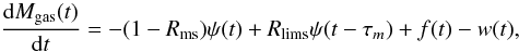 (1)where, Rms and Rlims are the masses returned to the ISM by massive- and low-intermediate mass stars, respectively. τm is the time delay of LIMS for their total gas ejection into the ISM, and ψ(t), f(t) and w(t) are the star-formation, accretion, and outflow rates as function of time, respectively.
In addition, the evolution of the gaseous mass in element i is  (2)
(2)
where  (t) and
  (t) are the abundances (by mass) of element i in the gas accreted and in the gas expelled from the galaxy, respectively. Ei(t) is the gas rate, in the element i, returned to the ISM by MS, LIMS, and SNIa that die at a time t, and it is calculated by
 ![Mathematical equation: \begin{eqnarray*} E_i&=&[{R}_{\rm ms} X_i(t) + {\rm y}_{i,\rm ms}]\psi(t)+[{R}_{\rm lims} X_i(t-\tau_i) + {\rm y}_{i,\rm lims}]\psi(t-\tau_i) \\ &&+{\rm y}_{i,\rm snia}\psi(t-\tau_{\rm snia}), \end{eqnarray*}](/articles/aa/full_html/2011/11/aa16957-11/aa16957-11-eq36.png) where τi is the time-delay when the group of LIMS enrich the ISM with the element i (see Franco & Carigi 2008) and τsnia is the time-delay of SNIa to pollute the gas mass of the galaxy.
where τi is the time-delay when the group of LIMS enrich the ISM with the element i (see Franco & Carigi 2008) and τsnia is the time-delay of SNIa to pollute the gas mass of the galaxy.
In Appendix A we present for the six initial stellar metallicities and two different upper mass limits of the initial mass function, τm, τi, Rms, Rlims, yms, ylims, and ysnia for the elements considered in this work.
3. Assumptions of the chemical evolution models
Below we describe in detail the assumptions included in our models.
-
1)
We adopt the mass-accretion rate proposed by CCP06, which was tailored to NGC 6822 from cosmological models of galaxy formation. Therefore, the accretion history is a better approximation for this galaxy than simple parametric equations. Carigi et al. (2006) described two families of cosmological models for the increase of baryonic mass: S (small-infall) and L (large-infall). We have chosen the L-models because they better adjust the observational constrains presented by CCP06 (the S-models predict higher enrichment in O/H and C/H than the L-models). In addition, we have parametrized the accretion history of the baryonic mass as a function of time, derived by CCP06. This parametrization, which is used for our chemical evolution models, is presented in Fig. 1 (upper panel) and is given by the expression
 (3)The accreted material is assumed to be primordial, that is, with a chemical composition given by X = 0.752, Y = 0.248, and Z = 0.000 as derived from WMAP observations by Dunkley et al. (2009) and for metal-poor irregular galaxies by Peimbert et al. (2007a);
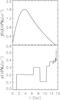
Fig. 1 Accretion (upper panel, see Eq. (3)) and star-formation (bottom panel, CCP06) histories adopted in the models. 13.5 Gyr corresponds to the present time.
-
2)
we consider the history of the star-formation rate (SFR) derived for NGC 6822 by CCP06 based on observed color-magnitude diagrams and photometric evolution models (Fig. 1, bottom panel). Interestingly, the accretion-mass history (shown in the upper panel of Fig. 1) and the SFR do not follow the same trend and seem to contradict each other in the latter 3 or 4 Gyr, when the accretion diminishes while the SFR increases abruptly. It should be considered, however, that the SFR should not follow the gas accretion closely because this accretion is only one of the mechanisms for increasing the SFR. On large scales, the formation of stars is controlled by an interplay between self-gravity and supersonic turbulence, operating on the gas already accreted. It is not clear how star-formation bursts are triggered in dwarf galaxies but for NGC 6822 Gouliermis et al. (2010) suggest that turbulence on kpc scales is the major agent that regulates star-formation. Several mechanisms have been proposed as able to produce turbulence on large scales. In particular, for NGC 6822 a possible mechanism that could have triggered at least the increase in the SFR during the last 100–200 Myr has been found in the presence of an apparently independent stellar structure called the “northwestern” companion, which is considered to be currently interacting with the main body of NGC 6822 and causing the tidal arms in the southeast of the galaxy (de Block & Walter 2000, 2003). If such an interaction occurred in the past (which is possible if the northwestern companion is a satellite nearby NGC 6822), it could have been the mechanism that triggered different starbursts in NGC 6822;
-
3)
we use the initial mass function (IMF) of Kroupa et al. (1993), in the 7.5 − MupM⊙ mass range for Z < 10-5 and in the 0.1 − MupM⊙ mass range for Z > 10-5. Mup is a free parameter adjusted to reproduce the observed O/H abundance ratio;
-
4)
we assume different stellar yields, depending on initial stellar mass (m) and on initial stellar metallicity Zi, provided by different authors. However, these yields do not cover the entire mass range. In the case of LIMS, we have a complete library from 1 M⊙ to 6 M⊙ and for MS, the mass range covered goes from 9 M⊙ to 80 M⊙. To fill the mass gap (from 6 M⊙ to 9 M⊙), we proceeded as follows: for the 6 < m/M⊙ ≤ 7.5 mass range we assigned the stellar yield values given by mass fraction (pi) of the 6 M⊙ star. In the same way, for the 7.5 < m/M⊙ < 9 mass range we assigned the pi values of the 9 M⊙ star.
Specifically,
-
4.1)
for LIMS we adopt the stellar yields by Karakas & Lattanzio (2007), and the integrated yields used by our model are given by
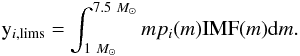 (4)The results for ten elements, five initial
stellar metallicities, and two different Mup values
are presented in Tables A.4 and A.5;
(4)The results for ten elements, five initial
stellar metallicities, and two different Mup values
are presented in Tables A.4 and A.5; -
4.2)
for MS we consider the stellar yields obtained from models for the pre-SN stage and the SN stage. The pre-SN yields are taken from the work of the Geneva-group (Maeder 1992; Meynet & Maeder 2002; Hirschi et al. 2005; Hirschi 2007). The SN yields are taken from Woosley & Weaver (1995) adopting their models B for the 12–30 M⊙ range and their models C for the 35–40 M⊙ range. We combine the Geneva group yields with the Woosley & Weaver yields using the prescription proposed by Carigi & Hernandez (2008), who connect the mass of the carbon-oxygen cores (MCO) from the Geneva group to MCO from Woosley & Weaver, using the prescription given by Portinari et al. (1998). Under these assumptions the He, C, N, and O yields are equal to the pre-SN ones, but for heavier elements the yields are similar to the SN ones. For m > 40 M⊙ the adopted yields for the heavier elements are similar to those given for m = 40 M⊙. The chemical contribution of MS is in IRA, and the integrated yields are given by
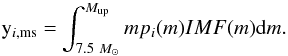 (5)The results for ten elements, six initial
stellar metallicities, and two different Mup values
are presented in Tables A.4 and A.5;
(5)The results for ten elements, six initial
stellar metallicities, and two different Mup values
are presented in Tables A.4 and A.5; -
4.3)
for SNIa we consider the stellar yields, Pi(snia), given in M⊙ by Nomoto et al. (1997), which are almost independent of the initial stellar metallicity. We assume that a fraction Abin of the stars with masses between 3 and 15 M⊙ corresponds to binary systems and that every one of these systems becomes a SNIa. Abin is a free parameter of the model, which is found by fitting the observed Fe/H ratio. We consider that all SNIa of each stellar generation enrich the interstellar medium at τsnia = 1 Gyr after the formation of SNIa progenitors (see Fig. 1 of Mannucci 2008). The integrated yields are given by
 (6)where
MB is the mass of the binary
system. yi,snia values for ten
i-elements and two different Mup
values are presented in Tables A.4 and A.5;
(6)where
MB is the mass of the binary
system. yi,snia values for ten
i-elements and two different Mup
values are presented in Tables A.4 and A.5;
-
4.1)
-
5)
the evolution of all the models is followed from an initial time, t0 = 0, to a final time, tf = 13.5 Gyr, with a step of Δt = 0.01 Gyr. The initial conditions in all models are Mgas(t0) = 0 and Mstar(t0) = 0;
-
6)
for the outflow rates we use two types of prescriptions:
-
6.1)
well-mixed winds. We assume that the ejecta of MS, LIMS, and SNIa are well-mixed with the ISM of the galaxy before part of the ISM is expelled into the intergalactic medium (IGM). We consider that well-mixed winds depend on the SFR and consequently the outflow rate is given by
 (7)where ν is a free parameter in
our models, adjusted to reproduce the observed Mgas
of the galaxy;
(7)where ν is a free parameter in
our models, adjusted to reproduce the observed Mgas
of the galaxy; -
6.2)
selective winds. We assume that during the time interval when a selective wind lasts, the ejecta produced by MS during that interval is expelled from the galaxy into the IGM without mixing with the ISM, therefore these ejecta do not contribute to the chemical enrichment of NGC 6822. The total mass lost owing to the selective winds is small relative to the gaseous mass of the galaxy.
-
6.1)
4. Models for abundances derived from collisionally excited lines
4.1. Observational constraints
NGC 6822 has been extensively studied along the years by different authors, therefore good observational constraints can be found in the literature. For instance, CCP0 derived its total dynamic, total baryonic, and gaseous masses. They amount to MT = (2.0 ± 0.5) × 1010 M⊙, Mbar = (4.3. ± 0.2) × 108 M⊙ and Mgas = (1.98 ± 0.2) × 108 M⊙, respectively.
The chemical abundances of several H ii regions, determined by diverse authors from collisionally excited lines (not corrected for dust depletion) were compiled by HPCG09, with the exception of Cl/H, which comes from Peimbert et al. (2005). The average O/H abundance of those H ii regions is 12 + log (O/H) = 8.08 ± 0.05, and HPCG09 found no evidence of chemical inhomogeneities in this galaxy for the H ii regions located in a central area of about 3 kpc in diameter. We will include a correction owing to depletion in dust grains by adding 0.08 dex to the O gaseous abundances of H ii regions; this correction has been suggested by Peimbert et al. (2005) as adequate for NGC 6822. From this we obtain 12 + log (O/H) = 8.16 ± 0.05. On the other hand, from A-type supergiant stars, Venn et al. (2001) derived the chemical abundance of iron to be 12 + log (Fe/H) = 7.01 ± 0.20. These data will be used as observational constraints for the present component of the ISM.
In addition, HPCG09 obtained the chemical abundances of 11 PNe. These authors found that some of the PNe are relatively young and their average O/H ratio (12 + log (O/H) = 8.11 ± 0.10) is similar to that of H ii regions. We tag these PNe as “young PNe”. Besides, there is a sample of PNe with much lower O, showing an average of 12 + log (O/H) = 7.72 ± 0.10. We tag these PNe as “old PNe”. The chemical abundances of both groups will be used in the chemical evolution models as additional constraints corresponding to the past and recent-past component of the ISM. No correction for dust is considered for PNe.
At the bottom of Table 1 we present the O/H, N/O, Ne/O, S/O, Cl/O, and Ar/O abundance ratio averages for the best-determined H ii regions (the correction for dust is included), young PNe and old PNe. There is no observational value for C/H obtained from CELs, so there is no observational constraint for C/O. Following Allen et al. (1998), we will assume the following ages for the two PN groups: between 0.1 and 1 Gyr for the young PN population and between 3 and 9 Gyr for the old one. The present age of the galaxy is assumed to be 13.5 Gyr. In this table we also present the Fe/H value by Venn et al. (2001) from A-type supergiants. Because most of the Fe in H ii regions and PNe is trapped in dust grains (Peimbert & Peimbert 2010; Shields 1978; Delgado-Inglada et al. 2009), we do not present the gaseous Fe/H abundance. In this table we do not show either He, C or N abundances for PNe because PN progenitors strongly modify these element abundances during their evolution. Consequently, He, C and N abundances in the PN envelopes are not representative of those values in the ISM at the formation time of PN progenitors and cannot be considered as constraints for a chemical evolution model. Moreover, Cl abundances of PNe are not shown in Table 1 because they were not determined by HPCG09.
4.2. The computed models
We computed four chemical evolution models using different upper-mass limits for the IMF and different galactic wind prescriptions reproduce the observed Mgas and the O/H values (corrected for dust depletion) obtained from CELs in H ii regions. We labeled them M1C to M4C. In Table 1 we present the characteristics and time evolution of these four models. In column 1 we list the model name; in Col. 2 the upper-mass limit for the IMF used in the model; in Col. 3 the corresponding wind prescription: “W” for well-mixed and “S” for selective wind; in Col. 4 the gaseous mass predicted by the model at the present time (i.e., 13.5 Gyr); in Col. 5 we list the time at which the chemical abundances are obtained, they correspond to the times adopted for H ii regions, young PNe, and old PNe; and in columns from 6 to 13 the predicted abundance ratios at the different times. As we mentioned in Sect. 4.1, in the three rows at the bottom of this table we include the observed values for H ii regions, young PNe and old PNe, which are used as observational constraints.
For model M1C we adopted an Mup of 60 M⊙ for the IMF (equal to the value adopted by CCP06 in their best model), and we did not include any outflow. From Table 1 it is evident that M1C grossly fails to fit Mgas because it predicts a gas mass ~4.5 times higher than the observed value.
Thus, to reduce the enormous difference between the Mgas predicted by model M1C and the observed value, we have computed model M2C with a well-mixed outflow during the early history of the galaxy. This was originally proposed by CCP06, who computed the evolution of gaseous thermal energy in the galaxy provided by the SFR under the assumption of no gas outflow (see their Fig. 7). These authors demonstrated that the accumulated thermal energy is much higher than the present binding energy, therefore much of that energy should have been thrown away through galactic winds. Carigi et al. (2006) gave several arguments to explain why the outflows that are needed to eliminate this excess in thermal energy likely occurred in the first few billion years of evolution (t < 5 Gyr) when the galaxy was less bounded (note that the binding energy of a galaxy is also a function of time and in the hierarchical cosmology, the potential wells of galaxies for a given present mass were shallower in the past). The gas outflow should have stopped when the binding and thermal energy came to an equilibrium.
In our model the well-mixed galactic wind is turned-on at t = 1.2 Gyr, when the star-formation starts and it lasts 5.3 Gyr, the time necessary for the ejected mass to be the maximum possible, leaving the minimum amount of gas required to maintain the SFR. During the wind phase a value ν = 6.67 in the outflow rate equation (Eq. (7)) was required. The evolution of the total baryonic mass and the gaseous mass in the galaxy, as a function of time, is shown in Fig. 2. These two quantities are directly related to the infall, SFR, and galactic wind. The dashed line is the time evolution of the Mgas (Ec. 1) and the solid line is the time evolution of the total baryonic mass (dMbar/dt = f(t) − w(t)).
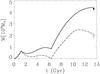 |
Fig. 2 Evolution of the total baryonic mass evolution (solid line) and gaseous mass (dashed line) used in our models M2C, M3C, M4C, and M1R. A well-mixed galactic wind occurs between 1.2 and 6.5 Gyr. Observational constraints are as in CCP06. |
Models that reproduce abundances calculated via collisional excited lines. The “W” and “S” are for well-mixed and selective wind prescription, respectively.
 |
Fig. 3 Chemical evolution of elements in NGC 6822 as predicted by model M4C. To reproduce the observed Mgas value and the different heavy element abundances obtained from collisionally excited lines for H ii regions, a well-mixed galactic wind lasting from 1.2 to 6.5 Gyr and an Mup = 40 M⊙ are assumed in this model. The O/H value of H ii regions has been corrected for dust depletion, as explained in Sect. 4.1. The filled circles, filled squares, and filled triangles represent the average observational values for H ii regions, young, and old PN populations, respectively. The filled star in the Fe/H panel represents the value derived by Venn et al. (2001) for A-type supergiant stars. Observed C/H value is not shown because there is no observed value from CELs. |
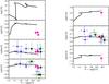 |
Fig. 4 Element abundance ratios relative to O as predicted for model M4C compared to observed values of PNe and H ii regions as presented in HPCG09. The O/H abundance of H ii regions was corrected for dust depletion, as explained in Sect. 4.1. H ii regions are represented by magenta filled circles, young-PNe by green filled squares and old-PNe, by blue filled triangles. The open squares are the two type-I PNe, and the open triangle is PN6 (see text or HPCG09). The magenta filled star in the Fe/O panel represents the value derived by Venn et al. (2001) for A-type supergiants. Observed C/O value is not shown because there is no observational C/H value from CELs. |
The present-time O/H value predicted by model M2C is 4σ higher than the observed values in H ii regions. Similarly, the ISM O/H ratio found at t = 12.9 Gyr is 2σ higher than the observed values of the young PN population, and for the old PN population the predicted ISM O/H value at t = 7.5 Gyr is 2.6σ higher than observed (see Table 1).
Therefore, to better reproduce the O/H abundance ratios we constructed model M3C by adding selective winds to the assumptions of model M2C. A selective wind where only the material produced by MS is expelled to the IGM might have been caused by the presence of a notable increase in the star-formation rate in the last 600 Myr, as reported by CCP06 and Gouliermis et al. (2010, and references therein). Model M3C required a selective wind between 12.5 and 13.5 Gyr to reproduce the current O/H value given by H ii regions. Therefore this model is identical to model M2C for t < 12 Gyr, but reproduces the observed O/H ratio well and it also reproduces the O/H values for both PN populations well. For the other elements that are produced by MS (Ne, Ar, Cl, and S) the predicted Xi/O ratios are similar in both models, unlike those elements partially produced by LIMS (C and N), for which the abundance ratios relative to O are slightly higher than in M2C owing to the loss of metals produced by MS in the selective wind phase (see Table 1). Although model M3C succeeds in fitting the observed O/H abundances, we do not consider it a satisfactory model because the physical mechanism to produce a 1 Gyr selective wind, where all chemical elements ejected by all MS are expelled to the IGM before they can mix with the ISM, is unlikely.
Then, to fit the O/H ratios observed in H ii regions, we proposed a lower value for Mup, keeping the other assumptions of model M2C (a similar model was proposed by HPCG09). For model M4C we used an Mup = 40 M⊙, including a well-mixed wind, starting at t = 1.2 Gyr and lasting 5.3 Gyr. Figure 3 shows the evolution predicted by model M4C for O, C, N, Ne, S, Cl, Ar, and Fe, relative to H, as a function of time. The thick lines (in the eight panels) represent the model results, the symbols represent the average values observed for H ii regions and the two PN populations as explained in the figure caption. We consider model M4C as our best model to reproduce the chemical abundances derived from CELs, therefore we will discuss its characteristics in the following subsection.
4.3. Our best model for abundances from CELs
Model M4C was tailored to fit the observed O/H abundance ratio by reducing Mup to 40 M⊙. We find that it also reproduces well the present abundances of the elements heavier than O. This Mup may be considered a low value for an IMF, but it seems a plausible value because some authors (e.g., Goodwin & Pagel 2005, and references therein) have argued that dwarf galaxies could have lower Mup values than that of the solar vicinity.
From the time evolution shown in Fig. 3 it is found that for all elements the temporal enrichment shows two minima, at 4 and 11 Gyr, owing to the dilution caused by the large infall and owing to the decrease of the SFR (see Fig. 1), respectively. We find that the predicted abundances of all elements at t ~ 7 Gyr agrees with the average abundances of old PNe, whose progenitors were formed at t = 7.5 ± 3.0 Gyr (6.0 ± 3.0 Gyr old). This epoch coincides with the beginning of the second fast enrichment. Furthermore, the recent abundances predicted for all elements matches within uncertainties (~0.1 dex) the average abundances of young PNe, whose progenitors were formed at t = 12.9 ± 0.5 Gyr (0.6 ± 0.5 Gyr old). In addition, Fig. 3 shows that model M4C matches well the H ii region average data of all elements within ~1.5σ (which corresponds to the uncertainties in abundance determinations), except in the case of N, where it fails grossly; this problem is discussed in more detail in the next paragraph. Finally, to fit the observed values of Fe/H, we needed to assume a fraction Abin = 0.01.
We remark that the model fails considerably in reproducing the presently observed N/H abundance ratio. This is found in several works on chemical evolution models (e.g., Chiappini et al. 2003; Carigi et al. 2005; Mollá et al. 2006; Romano et al. 2010; Kobayashi et al. 2011). The prediction of our model is 7.4σ higher than the value observed in H ii regions, therefore we consider that the N yields adopted for LIMS are in general overestimated the models.
To confirm the results given in the previous paragraphs, we present in Fig. 4 the C/O, N/O, Ne/O, S/O, Cl/O, Ar/O, and Fe/O abundance ratios as a function of 12 + log (O/H), predicted by model M4C. Here we show the data for the best observed objects published by HPCG09. H ii regions are presented as magenta filled circles, young-PNe are represented by green filled squares and old-PNe by blue filled triangles. The open squares are the two type-I PNe, and the open triangle is PN6 (in HPCG09 nomenclature) cataloged as an old-PNe based mainly on its Ar/H abundance. We remark that in this figure we present the most complete set of observational constraints for NGC 6822 to be compared with our chemical evolution model.
In this figure, regarding N/O, we find again that the model predicts to much N (probably because of problems with N yields). Unfortunately, we cannot comment about the C/H abundance because there are no determinations of this element using CELs.
In the case of Ne, all Ne/O ratios in PNe are above the H ii values and above model predictions. This could be caused by the ionization correction factor used to derive Ne (Ne/O = Ne++/O++ is commonly used), which is not adequate for low-ionization H ii regions or low-density PNe (Peimbert et al. 1992, 1995b). Ne/O from the model agrees better (within uncertainties) with the values for H ii regions, which means that the Ne and O yields for massive stars up to 40 M⊙, assumed in our model, are reliable.
The comparison is poor for S/O In particular, the model predictions are 2σ higher than the observed values in young PNe and H ii regions. The uncertainties in the S-abundance determinations are very large, in particular for PNe, therefore it is difficult to draw any conclusion regarding the S-yields.
For Cl/O our model agrees well with the present value of the ISM within the uncertainties. Similarly, the evolution of Ar/O agrees within the uncertainties with the observational values.
We reproduce the present Fe/H value obtained from A-type supergiant stars by assuming that only 1% of all stars between 3 M⊙ and 15 M⊙ become SNIa.
Model that reproduces abundances calculated via recombination lines plus correction for dust depletion. In Col. 3, “W” is for well mixed wind prescription.
5. Models for abundances derived from recombination lines
It is well known that the C++ and O++ abundances determined from the faint C ii and O ii recombination lines in photoionized nebulae are systematically larger than abundances derived from collisionally excited lines of the same ion (e.g., Rola & Stasinska 1994; Peimbert et al. 1995; Liu et al. 2004; Esteban et al. 2004; Tsamis et al. 2004; Wesson et al. 2005; Peimbert & Peimbert 2011; Simón-Díaz & Stasińska 2011; Tsamis et al. 2011; Carigi & Peimbert 2011). Other ionic abundances such as O+/H+ and N+/H+ derived from recombination lines show the same behavior. This problem is known as the “abundance discrepancy” and is generally parametrized by the abundance discrepancy factor (ADF), which is defined as  (8)Abundance discrepancy factors have commonly values of about 2. Then, trying to distinguish between the abundance ratios obtained from both CELs and RLs we have computed a model to reproduce the O/H abundance calculated from RLs and compared it with our best model based on collisionally excited lines (model M4C).
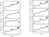 |
Fig. 5 Chemical evolution of elements in NGC 6822 as predicted by model M1R. To reproduce the observed Mgas value and the different heavy element abundance ratios obtained from RLs for H ii regions, a well-mixed galactic wind lasting from 1.2 to 6.5 Gyr and an Mup = 80 M⊙ are assumed in this model. The observed O/H and C/H values have been corrected for dust depletion, as explained in Sect. 4.1. The filled circles, filled squares, and filled triangles represent the average observational values for H ii regions, young, and old PN populations, respectively. The filled star in the Fe/H panel represents the value derived by Venn et al. (2001) for A-type supergiant stars. |
5.1. Observational constraints
We used the abundances reported by Peimbert et al. (2005) from RLs for the H ii region HV. These authors obtained a value 12 + log (O/H) = 8.42 ± 0.06, where this determination includes the correction for dust depletion. Peimbert et al. (2005) considered dust corrections of 0.08 dex for O and 0.10 for C, these corrections have been adopted for H ii regions throughout this paper. Abundance values for other elements are taken from Table 9 of Peimbert et al. (2005).
On the other hand, there are no abundance determinations based on RLs for PNe in NGC 6822 because these faint lines were not detected in these objects. Consequently, we have no direct observational constraints based on RLs for the past component of the ISM. Therefore we used the determinations of chemical abundances derived from CELs as reported by HPCG09 and modified them by considering a certain constant value for the ADF. Owing to this procedure, the RLs abundances for PNe should be considered as only indicative.
Liu et al. (2006) report that for most galactic PNe, ADFs are in the range of 1.6 to 3. Likewise, Peimbert et al. (1995a) determined ADFs for many galactic PNe and computed similar ADF values. Therefore we applied an ADF = 2 to the PN abundance determinations from CELs to derive a value for recombination lines. Note that the ratio of any heavy element to O in PNe is not affected by the ADF correction because the abundances of both elements were increased by the same amount.
In the bottom part of Table 2 we present the chemical abundances for H ii regions obtained via recombination lines plus correction for dust depletion. In addition we present the chemical abundances for the young and old PN populations calculated after using the ADF mentioned above for the abundance values by HPCG09.
5.2. The model
We computed a single chemical evolution model using similar assumptions to those described for model M4C. The model is labeled M1R and was tailored to reproduce the O/H abundance obtained for the H ii region HV from recombination lines.
As in model M4C, model M1R required a well-mixed wind starting at 1.2 Gyr and lasting 5.3 Gyr to reproduce Mgas. Now an Mup = 80 M⊙ is needed to reproduce the current O/H value. In Table 2 (top part) we present the gaseous mass and the O/H, C/O, N/O, Ne/O, S/O, Cl/O, Ar/O, and Fe/H ratios predicted by model M1R for different times.
In this model, the computed O/H value at t = 7.5 Gyr agrees very well with the adopted value for the old PN population. For the young PN population, the oxygen abundance calculated also agrees very well with the adopted value, which is very similar to the one in H ii regions. To fit the observed Fe/H value we required to adopt again Abin = 0.01.
Figure 5 shows the time evolution of the element abundances (O, C, N, Ne, S, Cl, Ar, and Fe) relative to H as predicted by model M1R. The thick lines in every panel represent our model results and the symbols are equal to those in Fig. 3. In this model the computed C/H value agrees well with the observational value obtained from RLs. The predicted N/H ratio is slightly closer to the observational constraint than in the model M4C, but it is still 3.6σ higher than the observed value, again indicating that the N yields for LIMS have to be revised. The predicted evolution of Ne/H shows relatively good agreement with observed values of old PNe, but not so good for young PNe and H ii regions. In the case of S/H, the predicted evolution agrees well with the PNe observed values, but not with observations of H ii regions. The predictions for Cl/H and Ar/H are significantly lower than the observed values in all the cases.
The described behaviors are clearly visible in Fig. 6, where we present the predicted evolution of the C/O, N/O, Ne/O, S/O, Cl/O, Ar/O, and Fe/O abundance ratios as a function of 12 + log O/H and the individual values of the best-observed objects (see Sect. 4.3). In this figure, many of the Ne/O observed values (in particular those of young PNe and H ii regions) lie above the predictions, the S/O for H ii regions is well-predicted within 1σ level. The predicted Cl/O and Ar/O values are ~ 2σ lower than the observed values. This latter problem is caused by the flat extrapolation assumed for the SN yields for m > 40 M⊙ (see Sect. 3). According to Woosley & Weaver (1995), Cl and Ar yields for m = 40 M⊙ are lower than for m = 35 M⊙ and therefore very massive stars would contribute less than massive stars to the ISM enrichment of those elements.
We consider for SN yields for m > 40 M⊙ are necessary a better comparison between models and observations. Recall that the yields in this paper for m > 40 M⊙ were extrapolated from the m = 40 M⊙ yields, and this extrapolation seems not adequate.
Finally, to fit the observed log [Fe/H] = − 0.49 value we adopted Abin=0.01, the same value used for CELs models.
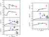 |
Fig. 6 Element abundance ratios, relative to O, as predicted for model M1R compared to observed values from recombination lines for the H ii region HV as presented in Peimbert et al. (2005) and the adopted values for PNe, as explained in Sect. 5.1. O and C abundances in HV was corrected for dust depletion, as explained in Sect. 4.1. H ii region HV is presented in magenta filled circles, young-PNe are represented by green filled squares and old-PNe, by blue filled triangles. The open squares are the two type-I PNe and the open triangle is PN6 (see HPCG09). The magenta filled star, in the Fe/O panel, represents the value derived by Venn et al. (2001) for A-type supergiant stars. |
5.3. The stellar yields problem
One of the most important elements in the chemical evolution models are the stellar yields. In the literature there are several works about stellar evolution models that present stellar yields computed from different codes. These stellar models include different physical ingredients and it is difficult to compare them (e.g., Romano et al. 2010, and references therein). In addition, there is no complete grid of stellar yields available for the entire range of stellar masses.
Our main problem to reproduce RLs observations for some chemical species is the lack of a homogeneous and complete set of stellar yields. First of all, as we explained in detail in Sect. 3, for LIMS we use the Karakas & Lattanzio (2007) yields, which cover from 1 to 6 M⊙ and for MS, those from the Geneva group (from 9 to 80 M⊙) for the pre-SN stage plus those from Woosley & Weaver (1995, hereafter WW) (for 9 to 40 M⊙) for the SN stage, together with the special treatment proposed by Carigi & Hernandez (2008). To reproduce the abundances from RLs, we need to extrapolate the WW yields from 40 M⊙ to 80 M⊙. We can see in Figs. 3 and 5 that the predictions for the evolution of O/H and Ne/H agree well with the observational constraints obtained from CELs (model M4C) and from RLs (model M1R) for the present (H ii regions) and past (PNe) components of the ISM. However, for the other chemical elements, C/H, N/H, S/H, Cl/H, Ar/H, and Fe/H the predictions do not change for the two models, even when for model M1R Mup is 80 M⊙.
Moreover, Cl/H and Ar/H values predicted by model M4C agree well with observations, but this is not the case for model M1R. We blame this on the lack of SN yields for masses > 40 M⊙ and the extrapolation made by us up to 80 M⊙. We have to keep in mind that Mup of the model M4C is equal to 40 M⊙ and no extrapolation for the yields was needed, while Mup of M1R is equal to 80 M⊙ and we had to extrapolate the yields.
Once we had these results, we did an exercise changing only the stellar yields of massive stars. We took the SN yields by Kobayashi et al. (2006) and the pre-SN yields by the Geneva group. We kept the rest of assumptions described in Sect. 3 and constructed two models, M4Ckoba (solid line) and M1Rkoba (dashed line) presented in Fig. 7.
We plot the evolution of the O/H, Ne/H, S/H, Cl/H, and Ar/H to compare them with the observations. The predictions for the evolution of Ne/H and S/H abundances agree very well with the observational constraints obtained from RLs only (dashed line and open symbols), but for CELs (solid line and filled symbols) the model predictions are ~3σ higher. Based on O/H, Ne/H and S/H, the Kobayashi et al. (2006) yields produce a good model for observed RLs abundances, but not for observed CELs abundances. If we want to force the M4Ckoba model to reproduce abundances from CELs, we must diminish Mup even more in the IMF (M4C has an Mup = 40 M⊙). The Cl/H and Ar/H predictions of both models are lower than the observational constraints, by ~0.75 and ~0.25 dex, respectively. To reproduce the Cl/H and Ar/H observed abundances in H ii regions, the Cl and Ar yields should be 5.6 and 1.8 times higher than those computed by Kobayashi et al. (2006). This is an important result, because previous works that tested stellar yields (e.g., Timmes et al. 1995; Romano et al. 2010; Kobayashi et al. 2011) were unable to check the Cl and Ar yields owing to the lack of abundance determinations of these elements in stars of the solar vicinity.
Based on this exercise, we prefer to keep the SN yields by WW for the model reproducing abundances from CELs (Mup = 40 M⊙). Nevertheless, we prefer the SN yields by Kobayashi et al. (2006) for the model reproducing RLs abundances (Mup = 80 M⊙) with Cl and Ar yields increased by factors of ~6 and ~2, respectively.
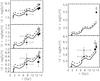 |
Fig. 7 The evolution for O/H, Ne/H, S/H Cl/H and Ar/H for two models, M4Ckoba (solid line) and M1Rkoba (dashed line), based on Kobayashi et al. (2006) yields. The filled circles, filled squares, and filled triangles represent the average observational values for H ii regions, young, and old PN populations, respectively. |
6. The ΔY/ΔO ratio and the IMF
Our chemical models predict the evolution of the He and O enrichment, both by mass, known as ΔY and ΔO, as a function of time. For convenience, and to compare with observations the ΔY /ΔO ratio is often used, where ΔO is equal to O and ΔY is equal to Y − Yp. Here Yp is the primordial He abundance and amounts to 0.248, the value derived from metal-poor irregular galaxies and WMAP (Peimbert et al. 2007a; Dunkley et al. 2009). It is well known that ΔY versus ΔO mainly depends on the adopted yields and the IMF.
Figure 8 shows the ΔY vs. ΔO behavior for our models M4C (solid line reproduces the O/H abundances given by CELs) and M1R (dashed line reproduces the O/H abundances given by RLs). Both lines show a similar behavior (same form, different slope), which depends mainly on the history of the mass accretion, the variation of the SFR with time, and on the time-delays assigned to the LIMS for their contribution to the chemical enrichment of He.
In Fig. 8 the initial slope corresponds to the first epochs of the galaxy, where only infall and IRA from MS are the processes that control the He and O abundances. The sudden discontinuity with a large increase in He occurs when LIMS start their contribution to the He enrichment of the ISM; these stars mainly produce He, but not O. From this point onward both curves evolve in a continuous increase of He and O, with an almost constant slope, perturbed only by a small loop, which occurs when the SFR changes suddenly in the epoch from 6.3 to 10.5 Gyr (see Fig. 1 bottom). At even later times both curves increase with an apparently constant slope.
Interestingly, although the behavior is similar, both curves showing the same perturbations owing the behavior of the SFR, the slopes are very different. As expected, the slope is steeper for M4C, which has Mup of 40 M⊙, and thus in this model less oxygen is produced. The slope derived for model M4C, considering only the zone from ΔO > 0.5 × 10⁻³, is about 7.2, while for model M1R it is about 3.7.
In Fig. 8 we also include two observational points. The filled square represents the (ΔY, ΔO) values derived from the He i RLs by Peimbert et al. (2005) and the [O iii] CEL (HPCG09) under the assumption of a constant temperature given by the [O iii] CELs. The open square represents the values derived from abundances obtained through He i and O ii RLs, considering the presence of spatial temperature variations. Evidently, in both cases ΔO is well-fitted because the models were tailored to fit O/H. On the other hand, the observed ΔY shows huge uncertainties, because it is very difficult to derive a precise value for He abundances because of i) the large statistical errors owing to the faintness of the lines (represented in the Fig. 8 by the error bars); and ii) the possible presence of neutral He in the observed H ii regions, which would increase the derived ΔY value for both determinations. Both Y values are derived from RLs, one under the assumption of constant temperature and the other under the assumption of the presence of temperature variations, the second one gives a Y value lower than the primordial value, probably indicating the presence of neutral helium inside the observed H ii region.
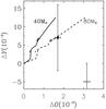 |
Fig. 8 Evolution of ΔY vs. ΔO for our two best models, M4C (solid line) and M1R (dashed line). The black square represents observed abundances under the assumption of constant temperature, and the open square represents abundances from RLs under the assumption of temperature variations (Peimbert et al. 2005), note that the observed ΔY values might be lower limits due to the possible presence of neutral helium inside the H ii region. |
We can also compare the slopes predicted by our models with observational data in the literature. For instance, Izotov et al. (2007) have derived chemical abundances for a large number of H ii galaxies of different metallicities. From these data they derived a slope ΔY/ΔO = 3.6 ± 0.7 or 3.3 ± 0.6, depending on the He i emissivities used, these numbers have not been corrected by the fraction of O atoms trapped in dust grains. By considering that this dust fraction amounts to 0.08 dex (Peimbert et al. 2005), we obtain from the Izotov et al. (2007) data that ΔY/ΔO = 3.0 ± 0.6 or 2.75 ± 0.5. On the other hand, Peimbert et al. (2007b), from theoretical and observational results, obtain ΔY/ΔO = 3.3 ± 0.7. These slopes agree better with model M1R, which was computed to fit O abundances from RL and for which an Mup = 80 M⊙ was assumed.
To summarize, model M1R produces a ΔY/ΔO slope similar to the one derived for a set of other galaxies, while M4C does not. In the case of NGC 6822, however, a much better Y determination is needed to discuss this problem further.
Time-delay (Gyr) of LIMS.
7. Discussion and conclusions
We have developed a code to calculate chemical evolution models for galaxies. The code includes the instant recycling approximation for MS, and a time-delay for the contribution of LIMS. This time-delay has been obtained for each element following the prescription given in Franco & Carigi (2008). Our code also includes the SNIa contribution to the chemical evolution in the galaxy. The code can be used for different SFRs, IMFs, yields, infalls and outflows. It predicts the evolution of 27 elements.
Using this code we calculated chemical evolution models for the dwarf irregular NGC 6822. The main characteristics of the models for this galaxy are
-
A time-dependent infall, parametrized from the one obtained byCCP06 from cosmological considerations, with a primordialabundance given byX = 0.752,Y = 0.248 andZ = 0.000(Fig. 1).
-
The star-formation history derived by CCP06, which is based on the photometric properties of the galaxy (Fig. 1).
-
The IMF by Kroupa et al. (1993) with different Mup values depending on the model.
-
A set of metallicity-dependent yields for 27 elements including H, He, C, N, O, Ne, S, Cl, Ar, Fe and others.
-
1% of the stars with masses between 3 and 15 M⊙ results in binary systems and every one of these systems becomes a SNIa. The contribution of SNIa enrich the ISM with a time-delay of 1 Gyr after the formation of the SNIa precursor.
-
Two types of time-dependent outflows can be used: well-mixed and selective.
Our models for NGC 6822 were constructed to fit the following observational constraints: a) Mgas; b) O/H chemical abundances of H ii regions and the Fe/H ratio of A-type supergiant stars representing the current abundances of the ISM; and c) chemical abundances of young (0.6 ± 0.5 Gyr) and old (6 ± 3 Gyr) planetary nebulae representing the abundances of the ISM at the time they were formed. The H ii abundances were corrected for the fraction of C and O in dust grains. Two sets of chemical abundances were used: those derived from CELs (HPCG09) and those derived from RLs (Peimbert et al. 2005), they differ by an abundance discrepancy factor, ADF, of about 0.26 dex. Because the RLs were not observed in PNe, we estimated their RL abundances based on the CEL abundances, and adopting an ADF of 2. Thus PNe abundances from RLs are only indicative.
The baryonic total mass captured by the system is given by the gas inflow estimated from cosmological considerations, and the amount of gas transformed into stellar mass is obtained from photometric data. From these two considerations only, the remaining gas turns out to be 4.5 times higher than observed. Therefore, to reproduce the observed Mgas value, the models required a well-mixed outflow lasting from t = 1.2 Gyr (which is the time when the star-formation starts) to t = 6.5 Gyr (when the gas mass has diminished sufficiently to fit the present gaseous mass, but without interrupting the star-formation, Fig. 2).
The SFR used in our models was derived from photometric data by CCP06, and agrees well with the abundances obtained for old PNe (HPCG09). These two studies are independent and therefore old PNe data support the SFR based on photometric data.
The two best models obtained to reproduce the present day ISM O/H value required a) an Mup = 40 M⊙ for model M4C, which is based on abundances derived from CELs, and b) an Mup = 80 M⊙ for model M1R, which is based on abundances derived from RLs.
Both models reproduce the O/H evolution of the past component of the ISM obtained from young and old PNe. This is particularly true for model M4C based on CELs. This result implies that the adopted SFR, derived from photometric data, describes the shape of the O/H evolution well and that the inferred well-mixed wind is consistent with the absolute O/H value.
The O/H ratio strongly depends on the use of RLs or CELs, but because the models are tailored to fit the observed values, it is not possible to decide which abundances are more adequate based on O/H alone.
We have tested the time evolution of other elements (C, N, Ne, S, Cl, Ar and Fe, relative to H). In general, the predictions of model M4C agree with the observations of H ii regions and old and young PNe, indicating that the assumptions used for this model are correct and that the SN yields used in the 9 to 40 M⊙ range, derived from WW, are adequate.
About 50% of C is produced by LIMS and about 50% by MS in the pre-SN phase. The C/O ratio is well-fitted by model M1R, a result that implies that the C and O yields are adequate.
On the other hand, the time evolution of heavy elements other than O, predicted by model M1R, do not always agree with the observations. Given that the predicted abundance ratios strongly depend on the yields, the adopted yields can then be tested. The C/O, S/O and Fe/O ratios predicted agree fairly well with the observations. But for Ne/O, Cl/O and Ar/O, the predicted values are lower than observed, probably indicating that the extrapolation of the SN yields from 40 to 80 M⊙ made in this paper is not good enough. A different set of yields for this mass range provided by Kobayashi et al. (2006) was tested, and we found a good agreement with observational values in both models (M4Ckoba and M1Rkoba, Fig. 7) for Ne/H and S/H, but Cl/H and Ar/H are underestimated by factors of ~ 6 and ~ 2 respectively. This is the first time that observational constraints for these elements are presented and compared with the models to test the stellar yields.
Returned mass and integrated yields for Mup = 40 M⊙.
Model M1Rkoba agrees very well with the observed value of O/H obtained from RLs, but to reproduce the observed value obtained from CELs (model M4Ckoba) it is necessary to lower Mup below 40 M⊙. We require a new set of yields for the 40 to 80 M⊙ mass range to make a better test of the model M1R against observations.
The predicted N/H values in both models are always considerably higher than observed and probably indicate that the N yields need improvement. About 80% of N is produced by LIMS and about 20% by MS in the pre-SN stage. Therefore, lower N yields for LIMS would provide a better fit to the observed N/O values.
At this point we are unable to conclude which set of abundances (based on CELs or RLs) represents the real abundances in the ISM better. Model M4C, which assumes Mup = 40 M⊙, reproduces well the O/H, Ne/H, S/H, Ar/H, Cl/H, and Fe/H observational constraints. While model M1R, which assumes Mup = 80 M⊙, reproduces well the O/H, C/H, Ne/H, S/H, and Fe/H observational constraints, but fails to reproduce Cl/H and Ar/H probably because of inadequate SN yields for stars with masses above 40 M⊙.
Returned mass and integrated yields assuming Mup = 80 M⊙.
Because ΔY does not depend strongly on the adopted temperature and ΔO does, ΔY/ΔO is a very good way to distinguish between M1R and M4C models. Unfortunately, the helium abundance determination for NGC 6822 is poor owing to the errors in the He I line intensities and the correction owing to the neutral He inside the H ii regions. We have used the ΔY/ΔO determinations derived by other groups, based on other galaxies, and we find that the M1R model agrees better with the observations of the other galaxies than the M4C model. A much more precise He abundance determination of the H ii regions in NGC 6822 is needed to advance in this topic.
Acknowledgments
We thank the referee Dr. G. Lanfranchi for his comments and suggestions, which helped to improve this paper significantly. We are grateful to Fátima Robles-Valdez for useful discussions. M. Peña is grateful to DAS, Universidad de Chile, for hospitality during a sabbatical stay when part of this work was performed. L.H.-M. benefited from the hospitality of the DAS, Universidad de Chile for this work. L.H.-M. received a scholarship from CONACYT-México and DGAPA-UNAM. M. Peña gratefully acknowledges financial support from FONDAP-Chile and DGAPA-UNAM. This work received financial support from CONACYT-México (grants 60354, 129753) and DGAPA-UNAM (grants IN-112708 and IN-105511).
References
- Allen, C., Carigi, L., & Peimbert, M. 1998, ApJ, 494, 247 [NASA ADS] [CrossRef] [Google Scholar]
- Buzzoni, A., Arnaboldi, M., & Corradi, R. L. M. 2006, MNRAS, 368, 877 [NASA ADS] [CrossRef] [Google Scholar]
- Carigi, L., & Hernández, X. 2008, MNRAS, 390, 582 [NASA ADS] [CrossRef] [Google Scholar]
- Carigi, L., & Peimbert, M. 2011, RMxAA, 47, 139 [NASA ADS] [Google Scholar]
- Carigi, L., Peimbert, M., Esteban, C., & García-Rojas, J. 2005, ApJ, 623, 213 [NASA ADS] [CrossRef] [Google Scholar]
- Carigi, L., Colín, P., & Peimbert, M. 2006, ApJ, 644, 924 (CCP06) [NASA ADS] [CrossRef] [Google Scholar]
- Chiappini, C., Romano, D., & Matteucci, F. 2003, MNRAS, 339, 63 [NASA ADS] [CrossRef] [Google Scholar]
- de Blok, W. J. G., & Walter, F. 2000, ApJ, 537, 95 [Google Scholar]
- de Blok, W. J. G., & Walter, F. 2003, MNRAS, 341, 39 [Google Scholar]
- Delgado-Inglada, G., Rodríguez, M., Mampaso, A., & Viironen, K. 2009, ApJ, 694, 1335 [NASA ADS] [CrossRef] [Google Scholar]
- Dunkley, J., Komatsu, E., Nolta, M. R., et al. 2009, ApJS, 180, 306 [NASA ADS] [CrossRef] [Google Scholar]
- Esteban, C., Peimbert, M., García-Rojas, J., et al. 2004, MNRAS, 355, 229 [NASA ADS] [CrossRef] [Google Scholar]
- Franco, I., & Carigi, L. 2008, RMxAA, 44, 311 [NASA ADS] [Google Scholar]
- Gieren, W., Pietrzyński, G., Nalewajko, K., et al. 2006, ApJ, 647, 1056 [Google Scholar]
- Goodwin, S. P., & Pagel, B. E. J. 2005, MNRAS, 359, 707 [NASA ADS] [CrossRef] [Google Scholar]
- Gouliermis, D. A., Schmeja, S., Klessen, R. S., et al. 2010, ApJ, 725, 1717 [NASA ADS] [CrossRef] [Google Scholar]
- Hernández-Martínez, L. 2010, Ph.D. Thesis, Universidad Nacional Autónoma de México [Google Scholar]
- Hernández-Martínez, L., Peña, M., Carigi, L., & García-Rojas, J. 2009, A&A, 505, 1027 (HPCG09) [NASA ADS] [CrossRef] [EDP Sciences] [Google Scholar]
- Hirschi, R. 2007, A&A, 461, 571 [NASA ADS] [CrossRef] [EDP Sciences] [Google Scholar]
- Hirschi, R., Meynet, G., & Maeder, A. 2005, A&A, 433, 1013 [NASA ADS] [CrossRef] [EDP Sciences] [Google Scholar]
- Izotov, Y. I., Thuan, T. X., & Stasińska, G. 2007, ApJ, 662, 15 [NASA ADS] [CrossRef] [Google Scholar]
- Karakas, A., & Lattanzio, J. C. 2007, PASA, 24, 103 [NASA ADS] [CrossRef] [Google Scholar]
- Kobayashi, C., Umeda, H., Nomoto, K., Tominaga, N., & Ohkubo, T. 2006, ApJ, 653, 1145 [NASA ADS] [CrossRef] [Google Scholar]
- Kobayashi, C., Karakas, A. I., & Umeda, H. 2011, MNRAS, 414, 3231 [NASA ADS] [CrossRef] [Google Scholar]
- Kroupa, P., Tout, C. A., & Gilmore, G. 1993, MNRAS, 262, 545 [NASA ADS] [CrossRef] [Google Scholar]
- Liu, Y., Liu, X.-W., Barlow, M. J., & Lou, S.-G. 2004, MNRAS, 353, 1251 [NASA ADS] [CrossRef] [Google Scholar]
- Liu, X.-W., Barlow, M. J., Zhang, Y., Bastin, R. J., & Storey, P. J. 2006, MNRAS, 368, 1959 [NASA ADS] [CrossRef] [Google Scholar]
- Maciel, W. J., Lago, L. G., & Costa, R. D. D. 2006, A&A, 453, 587 [NASA ADS] [CrossRef] [EDP Sciences] [Google Scholar]
- Maeder, A. 1992, A&A, 264, 105 [NASA ADS] [Google Scholar]
- Mannucci, F. 2008, ChJAS, 8, 143 [NASA ADS] [Google Scholar]
- Meynet, G., & Maeder, A. 2002, A&A, 390, 561 [NASA ADS] [CrossRef] [EDP Sciences] [Google Scholar]
- Mollá, M., Vílchez, J. M., Gavilán, M., Díaz, A. I. 2006, MNRAS, 372, 1069 [NASA ADS] [CrossRef] [Google Scholar]
- Nomoto, K., Iwamoto, K., Nakasato, N., et al. 1997, NuPhA, 621, 467 [NASA ADS] [Google Scholar]
- Pagel, B. E. J. 1989, RMxAA, 18, 161 [Google Scholar]
- Peimbert, A., & Peimbert, M. 2010, ApJ, 724, 791 [NASA ADS] [CrossRef] [Google Scholar]
- Peimbert, A., Peimbert, M., & Ruiz, M. T. 2005, ApJ, 634, 1056 [NASA ADS] [CrossRef] [Google Scholar]
- Peimbert, M., & Peimbert, A. 2011, RMxAASC, in press [arXiv:0912.3781] [Google Scholar]
- Peimbert, M., Torres-Peimbert, S., Ruiz, M. T. 1992, RMxAA, 24, 155 [Google Scholar]
- Peimbert, M., Torres-Peimbert, S., & Luridiana, V. 1995a, RMxAA, 31, 131 [Google Scholar]
- Peimbert, M., Luridiana, V., & Torres-Peimbert, S. 1995b, RMxAA, 31, 147 [Google Scholar]
- Peimbert, M., Luridiana, V., & Peimbert, A. 2007a, ApJ, 666, 636 [NASA ADS] [CrossRef] [Google Scholar]
- Peimbert, M., Luridiana, V., Peimbert, A., & Carigi, L. 2007b, ASPC, 374, 81 [Google Scholar]
- Portinari, L., Chiosi, C., & Bressan, A. 1998, A&A, 334, 505 [NASA ADS] [Google Scholar]
- Richer, M. G., & McCall, M. 2007, ApJ, 658, 328 [NASA ADS] [CrossRef] [Google Scholar]
- Rola, C., & Stasińska, G. 1994, A&A, 282, 199 [NASA ADS] [Google Scholar]
- Romano, D., Karakas, A. I., Tosi, M., & Matteucci, F. 2010, A&A, 522, A32 [NASA ADS] [CrossRef] [EDP Sciences] [Google Scholar]
- Serrano, A., & Peimbert, M. 1983, RMxAA, 8, 117 [Google Scholar]
- Shields, G. A. 1978, ApJ, 219, 559 [NASA ADS] [CrossRef] [Google Scholar]
- Simón-Díaz, S., & Stasińska, G. 2011, A&A, 526, A48 [NASA ADS] [CrossRef] [EDP Sciences] [Google Scholar]
- Talbot, R. J. Jr., & Arnett, W. D. 1971, ApJ, 170, 409 [NASA ADS] [CrossRef] [Google Scholar]
- Timmes, F. X., Woosley, S. E., & Weaver, T. A. 1995, ApJSS, 98, 617 [NASA ADS] [CrossRef] [Google Scholar]
- Tinsley, B. M. 1974, ApJ, 192, 629 [NASA ADS] [CrossRef] [Google Scholar]
- Tsamis, Y. G., Barlow, M. J., Liu, X.-W., Storey, P. J., & Danziger, I. J. 2004, MNRAS, 353, 953 [NASA ADS] [CrossRef] [Google Scholar]
- Tsamis, Y. G., Walsh, J. R., Vílchez, J. M., & Péquignot, D. 2011, MNRAS, 412, 1367 [NASA ADS] [Google Scholar]
- Venn, K. A., Lennon, D. J., Kaufer, A., et al. 2001, ApJ, 625, 754 [Google Scholar]
- Wesson, R., Liu, X.-W., & Barlow, M. J. 2005, MNRAS, 362, 424 [NASA ADS] [CrossRef] [Google Scholar]
- Woosley, S. E., & Weaver, T. A. 1995, ApJS, 101, 181 [NASA ADS] [CrossRef] [Google Scholar]
Appendix A
In this section we present the returned masses, time delays, and integrated yields for the chemical elements considered in this work.
In Table A.1 we show the time-delays of LIMS for the returned mass and for the integrated yields of eight chemical elements. These data are independent of the Mup value adopted in the IMF, but they are dependent on the initial stellar metallicity Zi.
The data shown in Tables A.2 and A.3 were obtained by assuming Mup = 40 M⊙ and Mup = 80 M⊙, respectively.
All Tables
Models that reproduce abundances calculated via collisional excited lines. The “W” and “S” are for well-mixed and selective wind prescription, respectively.
Model that reproduces abundances calculated via recombination lines plus correction for dust depletion. In Col. 3, “W” is for well mixed wind prescription.
All Figures
|
Fig. 1 Accretion (upper panel, see Eq. (3)) and star-formation (bottom panel, CCP06) histories adopted in the models. 13.5 Gyr corresponds to the present time. |
| In the text | |
|
Fig. 2 Evolution of the total baryonic mass evolution (solid line) and gaseous mass (dashed line) used in our models M2C, M3C, M4C, and M1R. A well-mixed galactic wind occurs between 1.2 and 6.5 Gyr. Observational constraints are as in CCP06. |
| In the text | |
|
Fig. 3 Chemical evolution of elements in NGC 6822 as predicted by model M4C. To reproduce the observed Mgas value and the different heavy element abundances obtained from collisionally excited lines for H ii regions, a well-mixed galactic wind lasting from 1.2 to 6.5 Gyr and an Mup = 40 M⊙ are assumed in this model. The O/H value of H ii regions has been corrected for dust depletion, as explained in Sect. 4.1. The filled circles, filled squares, and filled triangles represent the average observational values for H ii regions, young, and old PN populations, respectively. The filled star in the Fe/H panel represents the value derived by Venn et al. (2001) for A-type supergiant stars. Observed C/H value is not shown because there is no observed value from CELs. |
| In the text | |
|
Fig. 4 Element abundance ratios relative to O as predicted for model M4C compared to observed values of PNe and H ii regions as presented in HPCG09. The O/H abundance of H ii regions was corrected for dust depletion, as explained in Sect. 4.1. H ii regions are represented by magenta filled circles, young-PNe by green filled squares and old-PNe, by blue filled triangles. The open squares are the two type-I PNe, and the open triangle is PN6 (see text or HPCG09). The magenta filled star in the Fe/O panel represents the value derived by Venn et al. (2001) for A-type supergiants. Observed C/O value is not shown because there is no observational C/H value from CELs. |
| In the text | |
|
Fig. 5 Chemical evolution of elements in NGC 6822 as predicted by model M1R. To reproduce the observed Mgas value and the different heavy element abundance ratios obtained from RLs for H ii regions, a well-mixed galactic wind lasting from 1.2 to 6.5 Gyr and an Mup = 80 M⊙ are assumed in this model. The observed O/H and C/H values have been corrected for dust depletion, as explained in Sect. 4.1. The filled circles, filled squares, and filled triangles represent the average observational values for H ii regions, young, and old PN populations, respectively. The filled star in the Fe/H panel represents the value derived by Venn et al. (2001) for A-type supergiant stars. |
| In the text | |
|
Fig. 6 Element abundance ratios, relative to O, as predicted for model M1R compared to observed values from recombination lines for the H ii region HV as presented in Peimbert et al. (2005) and the adopted values for PNe, as explained in Sect. 5.1. O and C abundances in HV was corrected for dust depletion, as explained in Sect. 4.1. H ii region HV is presented in magenta filled circles, young-PNe are represented by green filled squares and old-PNe, by blue filled triangles. The open squares are the two type-I PNe and the open triangle is PN6 (see HPCG09). The magenta filled star, in the Fe/O panel, represents the value derived by Venn et al. (2001) for A-type supergiant stars. |
| In the text | |
|
Fig. 7 The evolution for O/H, Ne/H, S/H Cl/H and Ar/H for two models, M4Ckoba (solid line) and M1Rkoba (dashed line), based on Kobayashi et al. (2006) yields. The filled circles, filled squares, and filled triangles represent the average observational values for H ii regions, young, and old PN populations, respectively. |
| In the text | |
|
Fig. 8 Evolution of ΔY vs. ΔO for our two best models, M4C (solid line) and M1R (dashed line). The black square represents observed abundances under the assumption of constant temperature, and the open square represents abundances from RLs under the assumption of temperature variations (Peimbert et al. 2005), note that the observed ΔY values might be lower limits due to the possible presence of neutral helium inside the H ii region. |
| In the text | |
Current usage metrics show cumulative count of Article Views (full-text article views including HTML views, PDF and ePub downloads, according to the available data) and Abstracts Views on Vision4Press platform.
Data correspond to usage on the plateform after 2015. The current usage metrics is available 48-96 hours after online publication and is updated daily on week days.
Initial download of the metrics may take a while.