| Issue |
A&A
Volume 535, November 2011
|
|
|---|---|---|
| Article Number | A23 | |
| Number of page(s) | 12 | |
| Section | Astronomical instrumentation | |
| DOI | https://doi.org/10.1051/0004-6361/201116882 | |
| Published online | 26 October 2011 | |
Multiperiodicity, modulations and flip-flops in variable star light curves
I. Carrier fit method
1
Tartu Observatory, 61602 Tõravere, Estonia
e-mail: This email address is being protected from spambots. You need JavaScript enabled to view it.
2 Department of Physics, Gustaf Hällströmin katu 2a ( PO Box 64), 00014 University of Helsinki, Finland
Received: 14 March 2011
Accepted: 13 September 2011
Abstract
Context. The light curves of variable stars are commonly described using simple trigonometric models, that make use of the assumption that the model parameters are constant in time. This assumption, however, is often violated, and consequently, time series models with components that vary slowly in time are of great interest.
Aims. In this paper we introduce a class of data analysis and visualization methods which can be applied in many different contexts of variable star research, for example spotted stars, variables showing the Blazhko effect, and the spin-down of rapid rotators. The methods proposed are of explorative type, and can be of significant aid when performing a more thorough data analysis and interpretation with a more conventional method.
Methods. Our methods are based on a straightforward decomposition of the input time series into a fast “clocking” periodicity and smooth modulating curves. The fast frequency, referred to as the carrier frequency, can be obtained from earlier observations (for instance in the case of photometric data the period can be obtained from independently measured radial velocities), postulated using some simple physical principles (Keplerian rotation laws in accretion disks), or estimated from the data as a certain mean frequency. The smooth modulating curves are described by trigonometric polynomials or splines. The data approximation procedures are based on standard computational packages implementing simple or constrained least-squares fit -type algorithms.
Results. Using both artificially generated data sets and observed data, we demonstrate the utility of the proposed methods. Our interest is mainly focused on cases where multiperiodicity, trends or abrupt changes take place in the variable star light curves.
Conclusions. The presented examples show that the proposed methods significantly enrich the traditional toolbox for variable star researchers. Applications of the methods to solve problems of astrophysical interest will be presented in the next papers of the series.
Key words: stars: variables: general / methods: data analysis / methods: statistical
Deceased.
© ESO, 2011
1. Introduction
The light curves of variable stars can display very different modes of behaviour. They can be quite regular, often even periodic, or relatively fast changes can be detected. The methods to deal with such observed data can roughly be divided into two classes. The first class encompasses tools that are based on Fourier analysis methods, assuming that the light curve can be decomposed into a set of periodic (harmonic) components. The components themselves can then be interpreted as manifestations of, e.g., different pulsational modes (as in asteroseismology), rotation, orbiting, and so forth. The local behaviour of such multicomponent curves can be quite complex. For instance, it is quite easy to build simple examples where destructive interference between two nearby components with nearly equal frequencies allows some third component to dominate the observed curve. The detection of such local regularities often lead to the usage of the second type of analysis tools, usually referred to as the time-frequency analysis methods. Instead of a global model, a certain set of local variability elements is postulated, and then their change in time is followed. Probably the best known method of this kind is the wavelet transform.
For continuously observed signals the Fourier transform -based methods and different types of time-frequency transforms are a well-developed part of the traditional data processing work flow (see e.g. Poularikas 2010). The situation is different in the case of astronomical data. The irregular observing patterns and long time gaps in the measured series significantly complicate the analysis (see e.g. the review by Schwarzenberg-Czerny 2003, and references therein; or Chapter 5 in Aerts et al. 2010). For the first type of methods, the computed frequency spectra often show spurious peaks due to the regularities in the gap structure of the input data. The second class of methods, on the other hand, can only be used for the short, more or less continuous, subsets of data.
In this paper we propose a relatively new method, at least in the astronomical context, to deal with irregularly spaced data. We start from the simple physical assumption that even if an object is observed to exhibit irregular or semi-regular variability, some regular process can be identified in the background. The best example of this is stellar rotation, normally quite stable over long periods of time, the semi-regularity of the observed light curve being caused by inhomogeneities, such as dark spots, on the stellar surface. Another relevant setting is provided by accretion disks, where the Keplerian rotation of the accretion elements is more regular than the observed outflow of radiation. Using this assumption, we decompose the observed light curves into two components: a rapidly changing carrier tracing the regular part of the signal, and its slowly changing modulation. In this way, we construct a method combining both aspects of the two classes of methods presented above.
The proposed method is certainly not a new method to seek hidden periods from data with gaps and irregularities. Instead, we try to build continuous models for irregularly observed data using a priori known frequency. Proper visualization of the model can then help us to interpret the data at hand and to reveal possible physical effects. The method is of explorative nature and can be used as a starting point before building more sophisticated statistical, numerical or dynamical models.
The layout of the paper is somewhat non-traditional. Instead of commencing with a lengthy introduction and comparison of the new proposed method to various time series analysis methods that have been used in variable star research, we start with introducing the basic elements of the analysis method in Sect. 2, where we also give a detailed description of the algorithms used. Section 3 is dedicated to demonstrate the suitability of the proposed method in various astronomical settings, using both artificially generated and observational data sets. This allows the reader to get appreciation of the new method at work. In Sect. 4 we will give an overview of the related developments, discuss the new method in the light of previous work, and in Sect. 5 discuss the domains of its applicability. The full-scale application of the method to longer sets of observational data will be presented in the forthcoming papers in the series.
2. Carrier fit method
The notion of the carrier frequency is well known from communication theory. Very often this is just a single harmonic tone with a fixed frequency ν0. The carrier is modulated by a signal of interest and transmitted to receiver. In the receiver the modulated signal is demodulated and useful information is recovered. The simplest model for such a process is just a waveform  (1)where the carrier wave is modulated by two smooth low-frequency signal components a(t) and b(t). In some cases the signal can be represented in an analytic complex form
  (2)which allows the explicit tracking of the time dependent amplitude A(t), the phase ϕ(t), and most importantly, the instantaneous frequency
  (3)The real astronomical signals very often contain also higher harmonics of the basic frequency. Due to this we introduce, from the very beginning, a more complex model of the form
  (4)By including the term a0(t), we allow the mean level of the signal to be different from zero. We also assume that the total number of harmonics, K, is not very large.
2.1. The algorithm
To describe the details of the carrier fit method we start from the simplest model of a variable star light curve:  (5)where P0 is the period (measured in days) corresponding to the carrier frequency ν0 = 1/P0 (measured in cycles per day), and the two functions a(t) and b(t) describe slow changes of the curve. Here we define a slow process as one for which the characteristic changes of the functions a and b occur on time-scales significantly longer than the period of the carrier oscillation, P0.
To build approximation curves for the observed data we firstly need to have a proper value for the carrier period P0, the determination of which is discussed in detail in Sect. 2.5. Secondly, certain analytical or numerical models for the both slow modulating functions are required. These models themselves depend on certain sets of parameters, as discussed in Sects. 2.2 and 2.3 for the chosen two representations. After reliably determining P0 and formulating a suitable model for the modulators, the remaining task is to find the model that best fits the observations, and retrieve the corresponding parameters. This data fitting process itself can be formulated as a standard least-square approximation procedure. This procedure can, in general, involve both linear and non-linear parameters. Because of the overall complexity of non-linear fitting, we usually restrict our analysis to the linear regime.
Below we demonstrate the carrier fit tool using two different methods for smooth approximation of the modulators: trigonometric polynomials and splines. There are certainly many other possibilities – essentially every known method of data smoothing from literature can also be used in this context.
2.2. Trigonometric approximation
We start from the relatively transparent method of trigonometric approximation. This allows us to explicitly control the frequency domain behaviour of our algorithm.
Let the time interval [ tmin,tmax] be the full span of our input data. Then we can introduce a certain period D = C × (tmax − tmin) for which the coverage factor C is larger than unity (typically C = 1.1 − 1.5). Using the corresponding frequency, νD = 1/D, we can now build a trigonometric (truncated) series of the type:  (6)and
  (7)to be used as models for smooth modulating curves. The coverage factor C must be larger than the data span to avoid artefacts due to the built-in periodicity of our trigonometric models. Too large coverage factor leads to redundant parametrization. Very often the building of the trigonometric model starts from the rounding of the full span period, D, and checking that the coverage factor remains in reasonable limits. According to our definition of a slow process, the period D must be significantly longer than the carrier period P0.
Using basic trigonometric identities it is now easy to show that the full expansion of the carrier fit model will contain cosine and sine terms of the form  where l = 0,...,L. Proper expansion coefficient estimates must be computed for every term in the series for the fixed carrier frequency ν0 and “data frequency” νD; this is a standard linear estimation procedure and can be implemented using standard mathematical (statistical) packages.
In the beginning of our discussion about the algorithm, we started off with the simplest light curve model, Eq. (5), including only the lowest harmonic k = 1. To generalise to the full case, Eq. (4), including also higher harmonics, we will construct trigonometric representations ak(t) and bk(t) for each overtone of the carrier kν0, k = 1,...,K. The time dependence of a0(t) is also modelled using special trigonometric polynomial. If all polynomials use the same number of harmonics L and we approximate separate cycles by K-harmonic model, then the overall count of linear parameters to be fitted is N = (2 × L + 1) ∗ (2 × K + 1).
The actual choice of the representative parameters K and L depends on the particular object we are working with. The number of tones, K, depends on the complexity of the phase curves. The choice of L is constrained by the longest gaps in the time series. In principle, it is also possible to compute certain formal constraints using standard statistical regression theory (see Draper & Smith 1998). Very often the inspection of phase plots which are computed with different parameter sets can also be useful.
2.3. Spline approximation
The trigonometric models of the modulation curves are the most useful when the actual behaviour of the modulations is relatively continuous, i.e. without sharp transients. The spline approximations are more flexible from this point of view.
To build spline approximations we need to divide the full data time span into, say L, intervals. For every interval with index l = 1,...,L, and for each overtone of the carrier k = 1,...,K, we define two local sets of cubic curves  (8)and
  (9)to be used as local modulators for the different tones of the cosine and sine components of the carrier wave. The complete analytical model for the data will then consist of cosine components
  (10)and sine components
  (11)There will altogether be 2 × 4KL such components. To take into account the general level of the signal, we need to include also the unit component, after which the total number of modes to be fitted into data will be 8KL + 1. The splines are not just a sample of local polynomials, but must obey certain restrictions. In our simple case, we demand that the approximation curves themselves, their first and second derivatives should be continuous. As a result we need to complement our set of fitting equations with 2 × 3K(L − 1) linear constraints. The total number of free parameters will then be N = 2KL + 6K + 1. To perform the constrained least-squares fitting we used routines from the AS 164 -package written by Stirling (1981). The implemented algorithms are based on the so-called Givens rotations (see Gentleman 1973) and allow to solve weighted least-squares equations. The constraints are effectively taken into account by assigning infinite weights to the constraining equations.
2.4. Construction of an analytic signal
One of the useful properties of the carrier fit method is that it allows easily to compute Hilbert transforms for the model waveforms. Using the Bedrosian theorem (Bedrosian 1963), we can easily compute for term
 its Hilbert transform
  (12)By definition, the modulators a(t) and b(t) are smooth functions, or in spectral terms, their spectra are concentrated around the zero frequency. The carrier frequency is significantly higher, and therefore the modulators can be removed from the transform. The complex analytic signal (Gabor 1946) can now be constructed as
  (13)its amplitude as function of time
  (14)and the instantaneous frequency
  (15)can be computed. For the details we refer the reader to the paper by Vakman (1996).
Unfortunately the analytic signal approach is useful only for waveforms which are either completely or nearly harmonic. For more general curves the instantaneous values for amplitude, phase and frequency can be formally computed, but their interpretation is not straightforward.
2.5. Estimation of the carrier frequency
The most important input parameter for the carrier fit method is naturally the carrier frequency ν0, or the corresponding period P0 = 1/ν0 itself. Very often a useful value is already known from previous data analysis steps. Here are some typical cases:
-
estimate from previous literature is at hand;
orbiting period is known from eclipses;
rotation period is computed from radial velocity data (say, in fully synchronized binaries);
the period is estimated by averaging its seasonal values (Blazhko effect stars, spotted stars);
the central frequency of the band in the Fourier spectrum can be used (Quasi-Periodic Objects).
In the case when we do not have a proper value for carrier frequency we need to estimate it from the data. Next we formulate a method to compare different carrier frequencies, and describe how a rough initial value can be improved to eliminate any trends in phase plots.
The most natural choice to measure the quality of the carrier frequency value is to inspect the stability of the resulting light curve – with the optimal carrier frequency, the most stable behaviour should be obtained. For this purpose we can use the interpolated carrier fit trial waveform. Even if built using a very rough preliminary estimate for the frequency ν0, it approximates the input waveform in its entirety and is a continuous function. Let us fix a certain trial frequency νT somewhere around the preliminary carrier frequency ν0. We can divide the interpolated waveform into intervals of the length PT = 1/νT, and construct local phase curves  (16)where ti = t0 + iPT,i = 0,1,...,NT − 1 is a sequence of starting points of the different intervals of the interpolated curve
  , phase φ runs from 0 to 1, and NT is the total number of the intervals for a particular trial period. The phase curves change if we move along time (later we will plot such time-dependent curves as phase diagrams). We can now measure the rate of change of the phases along time using a statistic
  (17)Loosely speaking, we estimate the mean square of the first derivative of the phase diagram along time. The optimal value for carrier frequency should minimize our statistics (see the discussion in Sect. 3.9 and Fig. 22).
After computing the value for an optimal carrier frequency, we can recompute the curve estimates and repeat the optimal frequency search, and thereby obtain a refined value for the optimal carrier frequency. In actual computations such a procedure takes only a couple of iterations to converge. Using this approach, uncertainties in the initial value of the carrier frequency do not matter, as the method ultimately finds the optimal and consistent carrier. However, one problem can be identified with this procedure. The optimal carrier frequency, as defined above, is essentially only a representative device. Sometimes it may be hard to find a physical interpretation to the resulting carrier value computed from the data. Only if we can assume that behind the seemingly erratic variation of oscillation parameters there is a certain mean flow which can be characterized by a certain mean frequency, we can accept the solution as physically meaningful. Fortunately, in most practical cases, the carrier frequency is available from the very beginning or physical considerations lead to a proper interpretation easily.
2.6. Visualization
We use the following scheme to visualize our results. First we calculate a continuous curve estimate, , from the randomly spaced and gapped data set, using a carrier-based least-squares fitting scheme. This approximation is continuous and does not contain gaps, and therefore allows us to get a smooth picture of the long-term behaviour. Below we will discuss why and when we can trust such a gap-filling scheme. Next we divide this continuous curve into segments with a length of the carrier period  . Throughout the paper, we measure periods in the units of days, and frequencies in the units of cycles per day. We then normalize each segment so that the approximating values span the standard range of [ − 1,1] . After normalization, we stack the segments along the time axis. To enhance the obtained plot, we somewhat extend every segment along phases, so that the actual display is wider (along phases) than a single period. The normalization is a relevant part of our procedure because it helps to grasp phase information we are interested in (trends, drifts, flip-flops etc.). In the lower part of the plots we often depict the distribution of the actual observational time moments in the form of “bar code”. The black stripes correspond to the periods during which at least one observation is available. The bright stripes correspond to gaps. This method of visualization allows to verify that the model fits into the data and not into the gaps. If the number of nodes or harmonics L for the modulation model curves is chosen properly then the phase plots do not reveal underlying timing structure.
2.7. Local time-frequency analysis
The obtained continuous, “de-gapped” curve obtained by the carrier fit method can be used as an input to different additional analysis procedures. Now that a fully sampled data set has been obtained, the standard approaches are applicable, due to which many different choices are possible. For instance, we can compute local Fourier spectra for sliding time windows, or compute various wavelet transforms (see Poularikas 2010, for additional possibilities). The corresponding time-frequency plots can then be combined with phase diagrams to get full grasp of the changes in the underlying processes involved.
In particular, we use stacks of normalized, local in time, power spectra to reveal trends in frequency structure of artificial or observed curves.
3. Examples and applications
The carrier fit method is quite straightforward in its formulation and uses rather standard tools for its implementation. However, its full utility can be appreciated only by looking at some actual applications. To build up the required intuition, we first illustrate the method applying it to very simple analytical light curve models which are sampled at time points taken from real observations, and after that, to real astronomical data sets. In the current context, however, we totally ignore the physical background of the effects observed in each example star – our goal here is to show the versatility of the method.
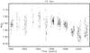 |
Fig. 1 V-band photometry of LQ Hya, JD 2 447 881–2 452 053. The longest time gap in the data set is 284 days. |
3.1. Timing sequences and data sets
To get realistic long-term photometric timing sequences we use a compilation of the V-band photometry for the variable star LQ Hya (Berdyugina et al. 2002). The used subset of 1627 points (displayed in Fig. 1) covers the interval JD 2 447 881–2 452 053 and contains rather long gaps (up to 284 days). In the most of the examples below we use only time points from this data set and calculate artificial time-dependent process values using analytical formulae. To model observational errors we add to each analytical time series value a noise component ε(t), which we generate as a normally distributed random variable with standard deviation of 5% from the overall series amplitude. This level of scatter is quite characteristic for reasonably good photometry, corresponding roughly to the signal-to-noise ratio of 20.
To demonstrate the suitability of the new methods to analyse the so-called Blazhko effect, we use the RR Lyr-type variable star MW Lyr. The data and detailed photometric solutions for the extensive photometry can be found in Jurcsik et al. (2008). As an input for reanalysis we used a well-sampled subset of the observations spanning over the interval JD 2 453 920–2 454 052, containing 3216 points (see Fig. 2).
The usability of the method in the context of the flip-flop phenomenon (e.g. Jetsu et al. 1993) is demonstrated using a subset of the extensive photometry of the rapidly rotating variable star FK Com, described in Korhonen et al. (2007) and depicted in Fig. 3. The data set contains 968 points and spans over the time interval JD 2 451 144–2 451 380.
The periods used as analytical model parameters are also taken to match some values that can be derived from observations; we return to their actual deduction from the data in the next papers of the series.
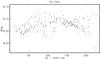 |
Fig. 3 V-band photometry of FK Com, JD 2 451 144–2 451 380. This is the only data fragment where the flip-flop phenomenon is observed continuously. |
3.2. Mismatched carrier frequency
Very often the appropriate carrier frequency ν0 is obtained from information which is available before the actual data processing. Being it rotation, orbiting or previously determined frequency, we need to confirm or re-evaluate it. To do this, a model with smoothly varying coefficients is fitted into the data, using the procedure described in Sect. 2.5. If the actual frequency is stable, but differs from the used carrier frequency we will see it from the time-dependent phase diagram. In the following example we use artificially generated data, but use the time-points from actual observations of LQ Hya described above. For instance, if the input model is just a single harmonic with a frequency ν = 0.149009 = 1/6.711001, magnitude offset and an added noise term ε(t) (see Sect. 3.1)  (18)then using a carrier value ν0 = 0.148714 = 1/6.724333, we will get a time-dependent phase diagram depicted in Fig. 4. To stress that the actual time points used in the analysis are taken from real observations with long gaps, we often plot a stripe-like illustration of the observing times on the lower part of the phase diagrams, as explained in detail in Sect. 2.6. With the refined-search method for the carrier frequency, we can recover the actual period in the input data set, after which the tilted stripes in the figure become strictly horizontal.
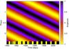 |
Fig. 4 Time-dependent phase diagram, i.e. the light curve amplitude profile over phase (y-axis) plotted as function of time (x-axis), for the mismatched carrier frequency example presented in Sect. 3.2. In this plot, a slightly too low carrier frequency of ν0 = 0.148714 is used, with K = 1 model and L = 8 modulation harmonics. Time points are obtained from real V-band photometric observations of LQ Hya; the bar-code in the bottom of the plot indicates when data has been available (black) and the gaps (bright). For visualization details see Sect. 2.6. |
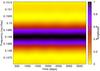 |
Fig. 5 Time-dependent local spectra computed for the interpolated curve |
To analyse time-dependent frequency spectra, we use the same continuous estimate, , but now we use it as an input to a standard time-frequency software1. In our particular case we compute frequency spectra for sliding time windows. After computing each local in time spectrum we again normalize it to span the standard range [ 0,1] . In this case the normalization helps us to track minor shifts in frequencies even if the amplitudes of the separate components change drastically. In this way our visualization method enhances the aspects of the variability which we are looking for. The result of this analysis is shown in Fig. 5.
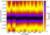 |
Fig. 6 Time-dependent local spectra computed for the original data points without interpolation, to be compared with Fig. 5. |
In principle it is possible to compute local frequency spectra for the original (not interpolated) data set. In Fig. 6 we depict the results of this kind of transform. From this plot it is evident how the gaps in the data tend to distort the overall image. The changes in the spectra can be (mistakenly) counted as real modulations.
3.3. Abrupt change in the period
The next interesting feature in variable star light curves is a possible jump in the frequency. Applying the same time points from observations as in the previous example, such a process can be described with a simple time series model 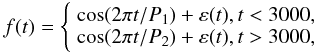 (19)where P1 = 6.747017, P2 = 6.701800, ε(t) is noise term described above (Sect. 3.1) We choose the carrier frequency, ν0, as a mean of the two model frequencies, and apply the carrier fit method to build a continuous curve
  ; the results are depicted in Fig. 7. As a comparison, local time-frequency analysis is made, the results of which are plotted in Fig. 8. The smooth appearance of the two plots is a result of the proper approximation scheme. The gaps of the input data are no longer visible, as they are properly filled in. This facilitates the visibility of the continuous patterns in the changing phase and period. However, if to compare the two plots, we see quite a relevant difference: the transition time from one period to the other is much longer for the time-dependent spectra if compared with the phase plot. To explain the difference, we need to take into account the fact that the time resolution of the transients differs for the two analysis methods. The smoothness of the phase plots is determined by the smoothness of the modulating coefficients a(t) and b(t), and can be adjusted using different fitting schemes. For time-dependent spectra the smoothness is controlled by the width of the sliding transform window. To obtain sufficient resolution in frequency domain we lose resolution in time domain. This is a well-known and ubiquitous uncertainty relation, and is common for all time-frequency analysis methods.
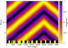 |
Fig. 7 The effect of an abrupt change in the period (Sect. 3.3) in the time-dependent phase diagram. The period before the jump is P1 = 6.747017, and after it P2 = 6.7018004. The used carrier is P0 = 6.724333, the number of model harmonics, K = 1, and the number of modulation harmonics, L = 8. |
 |
Fig. 8 The effect of an abrupt change in the period in the time-dependent local spectra; to be compared with Fig. 7. |
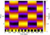 |
Fig. 9 The effect of two beating periods, P1 = 6.747017 and P2 = 6.701800, in the time-dependent phase diagram. The carrier used is P0 = 6.724333, the number of model harmonics K = 1, and the number of modulation harmonics L = 8. See Sect. 3.4. |
3.4. Two beating waves
Next we consider an example, where an interference between two nearby frequencies occurs. Again, the same time points with gaps as in the previous examples are used, and an artificial time series model of the form  (20)where P1 = 6.747017, P2 = 6.701800, and ε(t) is noise term (see Sect. 3.1), is analysed using the carrier fit method to build a phase diagram, plotted in Fig. 9, where a clear chessboard pattern can be seen. This can be understood by considering the trigonometric identity
 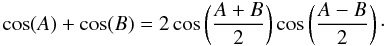 (21)The interference between the two nearby frequencies can be looked upon as a certain high-frequency main tone modulated by a low-frequency beat tone. In our case the beat period is ≈ 2000 days. Because we are dealing here with 100% modulation, the sign of the beat wave changes after every 1000 days, and the overall image of the time-dependent phase looks like a chessboard. These abrupt changes in the phase are somewhat unexpected if we take into account that the model contains only two simple harmonics. The carrier fit method and the used visualization technique allows us to reveal this natural flip-flop in the clearest way.
The continuous approximation curve can be further analysed by using the local time-frequency analysis method. The results of such an analysis with two different sliding windows are shown in Figs. 10 and 11. The first of these two figures, in which a sliding window of the length 600 days was used, demonstrates a very serious problem of the time-frequency analysis. From the form of the input model, we expect that two parallel lines along time are recovered. Instead, we see that the plot is dominated by a single maximum at a period which corresponds to the mean of the two model frequencies, and only around the locations, where the modulating beat wave changes sign, the spectrum splits into two separate frequencies. Even then the local maxima are not placed at the correct periods. Such a weird picture is due to the usage of a relatively short sliding time window (600 days) if to compare with beat period (2000 days). Even if we compute the local spectra for a four times longer time window (as in Fig. 11), there is still a slow wave seen in the positions of the two frequencies. This example illustrates a typical error made in time series analysis, where the original data is divided into segments, and each segment is analysed separately, after which conclusions are made according to the obtained local periods. Were the local spectra computed without a preceding continuous interpolation, the results could be even more misleading. In this particular case we consider the time-dependent phase plot a more appropriate analysis and visualization method.
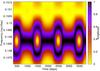 |
Fig. 10 The effect of two beating periods in the time-dependent local spectra, sliding window length is 600 days; to be compared with Fig. 9. |
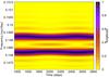 |
Fig. 11 The effect of two beating periods in the time-dependent local spectra, sliding window length is 2400 days; to be compared with Figs. 9 and 10. |
3.5. Linear trend in the frequency
As our next example of the carrier fit method, we define the input data as follows  (22)where
  moves linearly from 0 to 1 during the time span of the input data [ tmin,tmax] and ε(t) is a noise term (see Sect. 3.1).
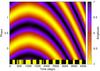 |
Fig. 12 The effect of a linear trend in frequency, as described in Sect. 3.5, in the time-dependent phase diagram. The used model parameters for the carrier fit read ν0 = 0.148714, K = 1, and L = 8. |
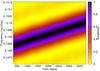 |
Fig. 13 The effect of a linear trend in frequency in the time-dependent local spectra. To be compared with Fig. 12. |
As seen from Fig. 12, the phase diagram for a curve with a changing frequency is rather complex, and it is not easy to interpret the actual form of the variability in the input data. In this case, however, the local time-frequency analysis reveals quite explicitly what is going on, as shown in Fig. 13.
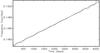 |
Fig. 14 The instantaneous frequency estimated using the Hilbert transform scheme of the carrier fit utility (thin line) over plotted with the analytical model (thick line) for the example presented in Sect. 3.5. Parameters for the carrier fit model: ν0 = 0.148714, K = 1 and L = 8. |
For this model, we can also apply an instantaneous frequency estimation scheme based on the Hilbert transform to construct an analytic signal, as described in Sect. 2.4. In Fig. 14, the computed run of the instantaneous frequency is displayed. Due to the noise component and gaps in the data set, the recovery is not exact. Also, the boundary effects in the beginning and end of the data are clearly visible, resulting from the extra freedom for the corresponding parts of the fitting curve. The results for this example also demonstrate an interesting aspect of time-frequency analysis. From Eq. (22) we can see that for the last time point, the frequency in the input data is 0.149214. The instantaneous frequency for this time point, recovered with both the local time-frequency analysis and Hilbert transform methods, is somewhat higher than the actual frequency. The fact observed here, the input data frequency and the recovered instantaneous frequency being not equal, is often overlooked (however, see Hempelmann 2002). The instantaneous frequency is not an entirely local value, but it also depends on its near neighbourhood due to the integral nature of the Hilbert transform.
3.6. Nonharmonic components
All the above examples were based on simple harmonic components. The real variable star light curves are seldom so simple. To show how the carrier fit method works for non-harmonic waveforms, we define a model with two interfering components f(t) = c1(t) + c2(t) + ε(t), where both components are of the form  (23)with the frequencies ν1 = 0.148214 and ν2 = 0.149214, respectively, corresponding to the periods used in the example of two beating waves, Sect. 3.4. From this example, it is useful to recall that the beat period of these two frequencies is roughly 2000 days. In this model, however, the two waveforms are “active” only during a half of their cycles.
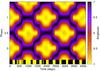 |
Fig. 15 The effect of the interference of non-harmonic waves with ν1 = 0.148214 and ν2 = 0.149214 in the time-dependent phase diagram for a carrier fit model using ν0 = 0.148714. See Sect. 3.6. |
It is quite clear that for the modelling of the process we need higher carrier harmonics. In Fig. 15 we show the results of the carrier fit with K = 3. Again, a regular pattern of minima and maxima is visible. If we compare with the simple beat pattern of Fig. 9, the most important difference is the occasional bi-modality of the phase curves. This is a result of an interplay between phases of the two “activity zones”. If the zones occur at phases nearby each other, we have curves with a single maximum; in case of roughly 180° separation, two maxima appear. For more complex waveforms, the interpretation of the phase plots can be even more convoluted.
3.7. Blazhko effect
As an example of an application of the carrier fit algorithm, based on trigonometric modulation curves, to real observational data, we re-analyse a subset of the photometry for the RR Lyr-type star MW Lyr, collected by Jurcsik et al. (2008). This pulsating star is known to exhibit a modulation of its light curve in addition to the variability due to the pulsations; this effect is known as the Blazhko effect. Jurcsik et al. (2008) proposed a bi-periodic model with the very accurate pulsational period of P0 = 0.397680 days modulated by a significantly longer period of Pb = 16.5462 days.
We start from a similar bi-periodic model with the frequencies kν0 + lνb, where k = 1,...,5 and l = −10,...,10, and ν0 = 1/P0 and νb = 1/Pb. The main difference to the original analysis by Jurcsik et al. (2008) is the usage of a smoother form of the basic waveforms (|k| ≤ 5 instead of |k| ≤ 13), and a more detailed modulation model (|l| ≤ 10 instead of |l| ≤ 4). The resulting normalized phase diagram is presented in Fig. 16.
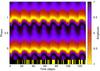 |
Fig. 16 Blazhko effect, phase diagram, bi-periodic fit with P0 = 0.397680 (K = 5), Pb = 16.5462 (L = 10). See Sect. 3.7. |
To apply the carrier fit method to the same input data sequence, we fixed the “data period”, D, to be 150 days with the coverage factor of C ≈ 1.14, so that the trigonometric modulation curves cover slightly more than the full data span. It is important to state that the resulting phase plot is not very sensitive to this number. We also set the number of harmonics K = 5 for the base frequency, and L = 10 for the modulations. In this way the system of linear equations to be fitted into the data was equal to the number of equations in the bi-periodic fit. The results are presented in a phase diagram of Fig. 17, showing a striking similarity of the phase patterns to the ones plotted in Fig. 16. An important point here is that the characteristic modulation pattern is revealed without pre-set (or precomputed) value for the modulation period. The only difference between the two diagrams is the somewhat larger number of small details for the bi-periodic fit and its exact periodicity. The phase diagram for the carrier fit solution is somewhat smoother and reveals minor fluctuations in the general periodic pattern. Whether these are fluctuations resulting form the observational noise, method artefacts, or sampling irregularities, remains currently open.
As this example clearly demonstrates, it is possible to recover the overall bi-periodic phase structure even without knowing the value of one of the periods.
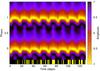 |
Fig. 17 Blazhko effect, phase diagram, carrier fit with P0 = 0.397680, D = 150, K = 5, and L = 10. To be compared with Fig. 16. |
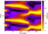 |
Fig. 18 FK Com flip-flop, phase diagram, carrier fit with trigonometric modulations, carrier ν0 = 2.40025, K = 3, L = 3, N = 49. See Sect. 3.8. |
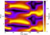 |
Fig. 19 FK Com flip-flop, phase diagram, carrier fit with spline modulations, carrier ν0 = 2.40025, K = 3, L = 5, N = 49. To be compared with Fig. 18. |
3.8. Flip-flop
To demonstrate the spline method in action, we performed both a trigonometric and spline-based fit into a subset of photometry of the star FK Com. A flip-flop phenomenon has earlier been detected in this very subset of data (Jetsu et al. 1993) covering one single observing season, during which a sharp jump of roughly 0.5 in phases occurs. The results of our analysis are shown in Figs. 18 and 19; for both the trigonometric and spline fits, the general picture is quite similar, and the abrupt jump in phase is clearly revealed. There are, however, some subtle differences. The trigonometric method is in a sense more “global”, due to which sharp features in one location can show up as oscillations somewhere far away. The spline method is essentially more “local”, and as a result the picture is somewhat smoother. We deliberately chose our parametrization here so that the total number of free parameters is equal for both methods.
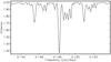 |
Fig. 20 The Stellingwerf’s statistic (criterion) for the input data with an abrupt change in the period (the same model as used in Sect. 3.3), the strongest minimum is at P0 = 6.7470. Note the overall complexity of the spectrum. See the discussion in Sect. 3.9. |
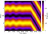 |
Fig. 21 Abrupt change in the period, phase diagram, P1 = 6.747017, P2 = 6.7018004, carrier P0 = 6.7470, K = 1, L = 8. See the discussion in Sect. 3.9. |
3.9. Computation of the carrier frequency
Finally, we illustrate the method to estimate the carrier frequency. Our input data model is the same as used in Sect. 3.3, Eq. (19), containing an abrupt change in the period. The noise added to the input data through the term ε(t) is now increased to 20% level. A fragment of a standard phase-dispersion spectrum (Stellingwerf 1978) for this data set is depicted in Fig. 20. The strongest peak is at a period P0 = 6.7470, coinciding closely with P1 in the input data model. This is to be expected, as the input data consists of a long fragment with this particular period. We proceed by using it as a carrier period value to build a time-dependent phase diagram depicted in Fig. 21. This carrier value produces a nearly horizontal stripe with some oscillatory behaviour for the part of the data having a period close to the used carrier, and a strongly tilted pattern for the part with a shorter period, already familiar from Sect. 3.2 for the case of a mismatched carrier frequency. The situation can be improved by refining the carrier frequency with a procedure described in Sect. 2.5 using the statistic D2 defined by Eq. (17), measuring the speed of changes in the phase diagram. For this example calculation, we plot this statistics in Fig. 22, showing a well-defined minimum at the frequency ν0 = 0.14850 = 1/6.7334. Using this frequency as the carrier, a time-dependent phase plot with minimum changes can be obtained, and is depicted in Fig. 23. Now the decreasing and increasing fragments of the phase diagram are well balanced.
Here we again note that the optimum carrier value is just a formal construct, and not based on any physical principle or insight. However, the procedure can be used as the last resort if no a priori information is available.
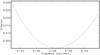 |
Fig. 22 Phase-change spectrum, statistic D2 (see Eq. (17)) is used as the criterion to estimate stationarity of the phase flow. See the discussion in Sect. 3.9. |
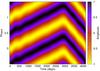 |
Fig. 23 Abrupt change in the period, phase diagrams, P1 = 6.747017, P2 = 6.7018004, carrier P0 = 6.7334, K = 1, L = 8. See the discussion in Sect. 3.9. |
4. Related work
Next we discuss the proposed algorithms in the context of the other well-known analysis methods for variable star light curves.
4.1. The O–C method
In the classical O–C (observed versus computed) method (see for instance Sterken 2005), the input light curve is divided into short fragments, so that for each fragment it is possible to securely determine a certain light curve event, most often a local minimum or maximum. For each event, a difference between the observed (O) and the computed (C) time moments is computed. The computed values are commonly just values from a periodic sequence  (24)where P is a period estimated beforehand, and E is an integer count of the full phases from the starting epoch T0. The differences O–C are then plotted for a full time span of the input data, and a proper model for the deviations is then sought for. Most often polynomial models are used.
In the carrier fit method proposed above, we are not very far off from this traditional scheme. The carrier period,  , is just an analogue of the period P in the equation for computed time point values. The fitting procedure itself tries to tightly model local fragments. In doing so, the local phase properties of the carrier wave indicate peculiarities of the original curve (minima and maxima among others). And finally, the smooth modulation curves are just analogues of the traditional polynomial models for O–C differences. In principle, it is even possible to modify the carrier fit method so that instead of trigonometric or spline models, simple polynomials are used as modulation curves.
The O–C method is often used to refine the already roughly estimated periods. As shown above, a mismatch in the carrier frequency reveals itself as a linear trend in the phase diagram. Therefore, to estimate the needed correction to the carrier period, the linear model for carrier modulations is considered sufficient.
The carrier fit method even shares the well-known problems of the O–C method. Most importantly – the wrong (or not exact enough) base period P can totally spoil the O–C analysis. This is also true when the choice of the proper carrier frequency is considered.
4.2. Fourier analysis
Methods based on, or connected to, standard Fourier analysis are certainly the most popular in variable star research. The classical series of papers, starting from Barning (1963), and ending with Koen (1990) and Frescura et al. (2008), gives a statistically sound treatment for the case when the input data can be described by a simple harmonic. The generalizations for non-harmonic (but periodic) and multiperiodic cases are obvious (see the chapter “Frequency Analysis” and references in the monograph by Aerts et al. 2010). For us the important point is that the classical methods are based on the assumption that the Fourier spectra of the underlying processes are discrete, and form a sparse set of frequencies. The sparseness of the spectrum makes it possible to recover the constituent waveforms from data sets with long gaps. Unfortunately, the periodicities caused by the gaps can be a source of serious problems. Along with every discrete peak in the original spectrum there will be a set of spurious peaks, and a perfect recovery can be a challenge.
Another method of frequency analysis is based on the idea of inversion. In this type of methods, the full discretized Fourier spectrum is fitted into data (see for instance Kuhn 1982, or more recently Nygrén & Ulich 2010). For a sensible inversion, the input data needs to be sampled quite densely. It must also be noted that inversion techniques involve huge matrix computations, and for this reason these methods fail to work for long input data sets.
The carrier fit algorithm described above combines properties of the discrete and continuous spectrum methods. First, we have a carrier frequency ν0 and its overtones kν0, which constitutes the discrete aspect. If the modulating waveforms ak(t) and bk(t) are smooth enough, the resulting spectrum will consist of K narrow but continuous frequency bands, accounting for the continuous aspect. By combining some good properties of the standard methods, we can achieve a compromise, where the discreteness of the midpoints of the narrow bands allow to “bridge” long gaps in time domain, and the continuity of the local spectra around the mid-frequencies allows to describe smooth time-dependent changes. Our method can essentially be regarded as a quite straightforward combination of the two classical approaches.
4.3. Local frequency analysis
There is another set of methods popular among variable star researchers. These methods are based on a division of the input data into separate segments, and then using some standard method to analyse them. The segmentation can be based on natural fragmentation of the input data or by formal division of the full data span. In some methods the segments can be overlapping in time (see recent detailed implementation by Lehtinen et al. 2011). It is assumed that the changes in the local Fourier spectra or other type statistics computed for different segments reveal actual trends in frequency structure of the underlying signal.
A typical example – the δ Scuti – type star θ Tuc was observed during six nights (Stobie & Shobbrook 1976), and data for each night was Fourier analysed seprately. The conclusion of the authors was
Photometric observations of θ Tucanae were Fourier analysed for their component frequencies. No coherent frequency could be found spanning the complete data set. It is shown that both the frequencies and amplitudes present in θ Tucanae change on time scale as short as 24 h.
However, more recent analysis of more extended data sets by other authors (for example Kurtz 1980; Paparó et al. 1996) gave another interpretation to the local variability of θ Tuc. It occurred that the varying local spectra result from constructive and destructive interferences of different coherent oscillation modes. The interpretation of the local spectra is further complicated by their low resolution. Above we gave an illustration of this effect (see Fig. 10) in the context of straightforward local Fourier analysis. This example shows that it is a good practice to use time-dependent phase diagrams (built by the carrier fit method) and time-dependent frequency analysis together to get a full understanding of the underlying process.
Localisation is carried to the limit in the method proposed by Tsantilas & Rovithis-Livaniou (2008). They use a very similar light curve model to Eq. (1)  (25)where observed data is decomposed into three continuous curves: amplitude a(t), frequency b(t) and phase c(t). The point estimates for the three components are then obtained by performing local non-linear least squares fits. Unfortunately, the presentation of the light curve in this form is not unique (for instance frequency changes can be compensated by phase changes) and consequently the obtained numerical results contain large amount of arbitrariness. In our method the carrier is fixed and modulations are constrained to be smooth. This allows to get more useful presentations for the light curves.
4.4. Time-frequency analysis
Another set of methods worthwhile to mention in this context are different time-frequency transforms. They are all based on a decomposition of the input data into set of sub-waves. Every sub-wave (in some methods called wavelet) is localized in time as well as in frequency. For a large set of this kind of decompositions we refer to a recent work by Blackman (2010) and references therein. In the context of variable star research, the most important problem with the standard time-frequency methods is related to the gaps in the input data. Usually the set of sub-waves is mathematically complete, but this leads to unrealistic “filling of gaps”. The sub-waves which are localized in short time intervals inside observing gaps will get zero values and as a result of that the structure of gaps will be seen through in the final two-dimensional spectrum. A very nice illustration of this point can be found in Szátmary (1994), where a large catalogue of model wavelet decompositions is given.
To overcome problems with gaps it is possible to modify the original wavelet method by making its resolution to depend on time. This can be achieved by the use of certain weighting schemes (see Foster 1996 for details) or adaptive wavelets, as done by Frick et al. (1997).
In the carrier fit method we use a priori information to constrain our sub-waves to be localised in fixed frequency strips around carrier and possibly around its harmonics. The shortcoming of our formulation is that our system of sub-waves is not complete. Nevertheless, with our algorithm, the gaps can be properly filled in, which enables to get a continuous phase or frequency diagrams that are more easy to interpret.
5. Discussion and conclusions
5.1. Utility of the carrier fit
All the simple examples above demonstrate that the carrier fit procedure itself is not sufficient to perform proper data analysis and interpretation. It is just a particular method to interpolate data sets with gaps to obtain a relatively smooth estimate for the variable star light curve. Interpolation itself has some value only when the real observed process and its observed values have certain properties. Most importantly, the process must be governed by some relatively stationary inherent clocking mechanism whose parameters change slowly. Fortunately this is the case for many variable stars.
5.2. Domain of applicability
By formulation and by algorithmic implementation the proposed utility can be considered as automatic. However, the obtained results can be very often misleading. This is why the complete understanding of the involved ideas is very important. Let us now reiterate major requirements for successful application of the carrier fit method.
Most importantly, the data to be analysed must come from an object with a certain internal clocking mechanism, being it rotation, orbiting or pulsation. This allows to fix, at least approximately, a proper value for a carrier frequency.
The modulating curves of the basic cycle must be relatively slow so that the spectral representations of the modulations and carrier frequency are located in different parts of the spectrum, i.e. the Bedrosian theorem is valid. It is also important that models for modulations must be smooth enough to allow “bridging the gaps” in observational sequences.
There must be enough of high quality observational points to allow adequate interpolation. To avoid over fit and under fit, standard methods from regression analysis should be used (Draper & Smith 1998).
The user of the methods must have a certain expertise to interpret the obtained phase diagrams. The proper and required intuition for that can be developed by using model computations with known input components. As a starting point the examples provided above can be useful.
Because the method involves inversion of large matrices, certain numerical problems may occur. The methods based on row-wise updating (Givens rotations) to solve the least-squares computational problems are very useful in this context; for details see Lawson & Hanson (1987).
The carrier fit method belongs to the class of data analysis methods called explorative. After getting an intuitively pleasing and convincing phase diagrams the researcher must quantify the results using more precise models (with proper estimates of errors etc.).
Another important aspect of the new method is the focus on phase behaviour. For that purpose, the visualization of normalized light curves is of great importance. This facilitates the detection of relevant trends and abrupt changes in light curves. This is just the aspect which usually remains hidden when standard multicomponent fit into the data is used.
In this paper we have presented a relatively new but simple class of data analysis methods which are useful in different astrophysical contexts. The best way to promote the methods would be their successful application to actual data sets. We are undertaking this effort in the next papers of the series.
The developed software is a part of the general time series package (Irregularly Spaced Data Analysis) which is freely available2
ISDA – Irregularly Spaced Data Analysis, available at http://www.aai.ee/~pelt/soft.htm
ISDA, http://www.aai.ee/~pelt/soft.htm, details by e-mail This email address is being protected from spambots. You need JavaScript enabled to view it.
Acknowledgments
Ilkka Tuominen sadly passed away on March 19, 2011. We wish to express our respect for his importance for the research on magnetically active stars. Financial support from the Academy of Finland grants 141017 and 218159 is acknowledged. We also thank the anonymous referee for useful comments on the manuscript.
References
- Aerts, C., Christensen-Dalsgaard, J., & Kurtz, D. W. 2010, Asteroseismology (Springer) [Google Scholar]
- Barning, F. J. M. 1963, B.A.N., 17, 22 [Google Scholar]
- Bedrosian, E. 1963, Proc. IEEE, 51, 868 [CrossRef] [Google Scholar]
- Berdyugina, S. V., Jankov, S., Ilyin, I., Tuominen, I., & Feckel, E. C. 1998, A&A, 334, 863 [NASA ADS] [Google Scholar]
- Berdyugina, S. V., Pelt, J., & Tuominen, I., A&A, 2002, 394, 505 [Google Scholar]
- Blackman, C. 2010, ApJS, 191, 185 [NASA ADS] [CrossRef] [Google Scholar]
- Draper, N. R., & Smith, H. 1998, Applied Regression Analysis, third edition (Wiley-Interscience) [Google Scholar]
- Foster, G. 1996, AJ, 112, 1709 [NASA ADS] [CrossRef] [Google Scholar]
- Frick, P., Baliunas, S. L., Galyagin, D., et al. 1997, ApJ, 483, 426 [NASA ADS] [CrossRef] [Google Scholar]
- Frescura, F. A. M., Engelbrecht, C. A., & Frank, B. S. 2008, MNRAS, 388, 1693 [NASA ADS] [CrossRef] [Google Scholar]
- Gabor, D. 1946, J. Inst. El. Eng., 93, 429 [Google Scholar]
- Gentleman, W. M. 1973, J. Inst. Maths. Applics., 12, 39 [CrossRef] [Google Scholar]
- Hempelmann, A. 2002, A&A, 388, 540 [NASA ADS] [CrossRef] [EDP Sciences] [Google Scholar]
- Jetsu, L., Pelt, J., & Tuominen, I. 1993, A&A, 278, 449 [NASA ADS] [Google Scholar]
- Jurcsik, J., Sódor, A., Hurta, Zs., et al. 2008, MNRAS, 391, 164 [NASA ADS] [CrossRef] [Google Scholar]
- Koen, C. 1990, ApJ, 348, 700 [NASA ADS] [CrossRef] [Google Scholar]
- Korhonen, H., Berdyugina, S. V., Hackman, T., et al. 2007, A&A, 476, 881 [NASA ADS] [CrossRef] [EDP Sciences] [Google Scholar]
- Kuhn, J. R. 1982, AJ, 87, 196 [NASA ADS] [CrossRef] [Google Scholar]
- Kurtz, D. W. 1980, MNRAS, 193, 61 [NASA ADS] [Google Scholar]
- Lawson, L. C., & Hanson, R. J. 1987, Solving Least Squares Problems, Society for Industrial Mathematics [Google Scholar]
- Lehtinen, J., Jetsu, L., Hackman, T., Kajatkari, P., & Henry, G. W. 2011, A&A, 527, A136 [NASA ADS] [CrossRef] [EDP Sciences] [Google Scholar]
- Nỳgren, T., & Ulich, Th. 2010, Ann. Geophys., 28, 1409 [NASA ADS] [CrossRef] [Google Scholar]
- Paparó, M., Sterken, C., Spoon, H. W. W., & Birch, P. V. 1996, A&A, 315, 400 [NASA ADS] [Google Scholar]
- Poularikas, A. D. 2010, Transforms and Applications Handbook, 3rd edn. (CRC Press) [Google Scholar]
- Rodonò, M., Messina, S., Lanza, A. F., Cutispoto, G., & Teriaca, L. 2000, A&A, 358, 624 [NASA ADS] [Google Scholar]
- Schwarzenberg-Czerny, A. 2003, ASP Conf. Ser., 292, 383 [Google Scholar]
- Stellingwerf, R. F. 1978, ApJ, 224, 953 [NASA ADS] [CrossRef] [Google Scholar]
- Sterken, C. 2005, in The Light Time Effect in Astrophysics, ed. C. Sterken, ASP Conf. Ser., 335, 3 [Google Scholar]
- Stobie, R. S., & Shobbrook, R. R. 1976, MNRAS, 174, 401 [NASA ADS] [Google Scholar]
- Stirling, W. D. 1981, Appl. Stat., 30, 204 [CrossRef] [Google Scholar]
- Szátmary, K., Vinkó, J., & Gál, J. 1994, A&AS, 108, 377 [NASA ADS] [Google Scholar]
- Tsantilas, S., & Rovithis-Livaniou, H. 2008, Comm. Astroseismol., 157, 87 [NASA ADS] [Google Scholar]
- Vakman, D. 1996, IEEE Transactions on Signal Processing, 44, 791 [NASA ADS] [CrossRef] [Google Scholar]
All Figures
|
Fig. 1 V-band photometry of LQ Hya, JD 2 447 881–2 452 053. The longest time gap in the data set is 284 days. |
| In the text | |
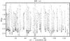 |
Fig. 2 V band photometry of MW Lyr, JD 2 453 920–2 454 052. |
| In the text | |
|
Fig. 3 V-band photometry of FK Com, JD 2 451 144–2 451 380. This is the only data fragment where the flip-flop phenomenon is observed continuously. |
| In the text | |
|
Fig. 4 Time-dependent phase diagram, i.e. the light curve amplitude profile over phase (y-axis) plotted as function of time (x-axis), for the mismatched carrier frequency example presented in Sect. 3.2. In this plot, a slightly too low carrier frequency of ν0 = 0.148714 is used, with K = 1 model and L = 8 modulation harmonics. Time points are obtained from real V-band photometric observations of LQ Hya; the bar-code in the bottom of the plot indicates when data has been available (black) and the gaps (bright). For visualization details see Sect. 2.6. |
| In the text | |
|
Fig. 5 Time-dependent local spectra computed for the interpolated curve |
| In the text | |
|
Fig. 6 Time-dependent local spectra computed for the original data points without interpolation, to be compared with Fig. 5. |
| In the text | |
|
Fig. 7 The effect of an abrupt change in the period (Sect. 3.3) in the time-dependent phase diagram. The period before the jump is P1 = 6.747017, and after it P2 = 6.7018004. The used carrier is P0 = 6.724333, the number of model harmonics, K = 1, and the number of modulation harmonics, L = 8. |
| In the text | |
|
Fig. 8 The effect of an abrupt change in the period in the time-dependent local spectra; to be compared with Fig. 7. |
| In the text | |
|
Fig. 9 The effect of two beating periods, P1 = 6.747017 and P2 = 6.701800, in the time-dependent phase diagram. The carrier used is P0 = 6.724333, the number of model harmonics K = 1, and the number of modulation harmonics L = 8. See Sect. 3.4. |
| In the text | |
|
Fig. 10 The effect of two beating periods in the time-dependent local spectra, sliding window length is 600 days; to be compared with Fig. 9. |
| In the text | |
|
Fig. 11 The effect of two beating periods in the time-dependent local spectra, sliding window length is 2400 days; to be compared with Figs. 9 and 10. |
| In the text | |
|
Fig. 12 The effect of a linear trend in frequency, as described in Sect. 3.5, in the time-dependent phase diagram. The used model parameters for the carrier fit read ν0 = 0.148714, K = 1, and L = 8. |
| In the text | |
|
Fig. 13 The effect of a linear trend in frequency in the time-dependent local spectra. To be compared with Fig. 12. |
| In the text | |
|
Fig. 14 The instantaneous frequency estimated using the Hilbert transform scheme of the carrier fit utility (thin line) over plotted with the analytical model (thick line) for the example presented in Sect. 3.5. Parameters for the carrier fit model: ν0 = 0.148714, K = 1 and L = 8. |
| In the text | |
|
Fig. 15 The effect of the interference of non-harmonic waves with ν1 = 0.148214 and ν2 = 0.149214 in the time-dependent phase diagram for a carrier fit model using ν0 = 0.148714. See Sect. 3.6. |
| In the text | |
|
Fig. 16 Blazhko effect, phase diagram, bi-periodic fit with P0 = 0.397680 (K = 5), Pb = 16.5462 (L = 10). See Sect. 3.7. |
| In the text | |
|
Fig. 17 Blazhko effect, phase diagram, carrier fit with P0 = 0.397680, D = 150, K = 5, and L = 10. To be compared with Fig. 16. |
| In the text | |
|
Fig. 18 FK Com flip-flop, phase diagram, carrier fit with trigonometric modulations, carrier ν0 = 2.40025, K = 3, L = 3, N = 49. See Sect. 3.8. |
| In the text | |
|
Fig. 19 FK Com flip-flop, phase diagram, carrier fit with spline modulations, carrier ν0 = 2.40025, K = 3, L = 5, N = 49. To be compared with Fig. 18. |
| In the text | |
|
Fig. 20 The Stellingwerf’s statistic (criterion) for the input data with an abrupt change in the period (the same model as used in Sect. 3.3), the strongest minimum is at P0 = 6.7470. Note the overall complexity of the spectrum. See the discussion in Sect. 3.9. |
| In the text | |
|
Fig. 21 Abrupt change in the period, phase diagram, P1 = 6.747017, P2 = 6.7018004, carrier P0 = 6.7470, K = 1, L = 8. See the discussion in Sect. 3.9. |
| In the text | |
|
Fig. 22 Phase-change spectrum, statistic D2 (see Eq. (17)) is used as the criterion to estimate stationarity of the phase flow. See the discussion in Sect. 3.9. |
| In the text | |
|
Fig. 23 Abrupt change in the period, phase diagrams, P1 = 6.747017, P2 = 6.7018004, carrier P0 = 6.7334, K = 1, L = 8. See the discussion in Sect. 3.9. |
| In the text | |
Current usage metrics show cumulative count of Article Views (full-text article views including HTML views, PDF and ePub downloads, according to the available data) and Abstracts Views on Vision4Press platform.
Data correspond to usage on the plateform after 2015. The current usage metrics is available 48-96 hours after online publication and is updated daily on week days.
Initial download of the metrics may take a while.