| Issue |
A&A
Volume 534, October 2011
|
|
|---|---|---|
| Article Number | A135 | |
| Number of page(s) | 8 | |
| Section | Cosmology (including clusters of galaxies) | |
| DOI | https://doi.org/10.1051/0004-6361/201117736 | |
| Published online | 20 October 2011 | |
Simulations of BAO reconstruction with a quasar Ly-α survey
1
CEA centre de Saclay, irfu/SPP, 91191 Gif-sur-Yvette, France
e-mail: This email address is being protected from spambots. You need JavaScript enabled to view it.
2
Institut d’Astrophysique de Paris, UMR7095 CNRS, Université Pierre et Marie Curie, 98 bis bd Arago, 75014 Paris, France
3
APC, 10 rue Alice Domon et Léonie Duquet, 75205 Paris Cedex 13, France
Received: 21 July 2011
Accepted: 30 August 2011
Abstract
Context. The imprint of baryonic acoustic oscillations (BAO) on the matter power spectrum can be constrained using the neutral hydrogen density in the intergalactic medium (IGM) as a tracer of the matter density. One of the goals of the baryon oscillation spectroscopic survey (BOSS) of the Sloan Digital Sky Survey (SDSS-III) is to derive the Hubble expansion rate and the angular scale from the BAO signal in the IGM. To this aim, the Lyman-α forest about 150 000 quasars will be observed in the redshift range 2.2 < z < 3.5 and over ~10 000 deg2.
Aims. We simulated the BOSS QSO survey to estimate the statistical accuracy on the BAO scale determination provided by such a large-scale survey. In particular, we discuss the effect of the poorly constrained estimate of the quasar’s unabsorbed intrinsic spectrum.
Methods. The volume of current N-body simulations being too small for such studies, we resorted to Gaussian random field (GRF) simulations. We validated the use of GRFs by comparing the output of GRF simulations with that of the Horizon-4Π N-body dark-matter-only simulation with the same initial conditions. Realistic mock samples of QSO Lyman-α forest were generated and their power spectrum computed and fitted to obtain the BAO scale. The rms of the results for 100 different simulations provides an estimate of the statistical error expected from the BOSS survey.
Results. We confirm the results from the Fisher matrix estimate. In the absence of error on the quasar’s unabsorbed spectrum, our simulations give an expected uncertainty of 2.3% for the BOSS quasar survey measurement of the BAO scale. The expected uncertainties for the transverse and radial BAO scales are 6.8% and 3.9%, respectively. The significance of the BAO detection is assessed by an average Δχ2 = 17 but Δχ2 ranges from 2 to 35 for individual realizations. The error on the quasar’s unabsorbed spectrum increases the error on the BAO scale by 10 to 20% and results in a subpercent bias.
Key words: method: numerical / large-scale structure of Universe / dark energy / quasars: absorption lines / intergalactic medium
© ESO, 2011
1. Introduction
Constraining properties of the dark energy that drives the expansion of the Universe is the key to understanding cosmology. Baryonic acoustic oscillations (BAO) in the pre-recombination baryon-photon fluid generate a bump in the matter correlation function at a distance corresponding to the sound horizon at decoupling (Peebles & Yu 1970; Sunyaev & Zeldovich 1970; Eisenstein & Hu 1998; Bashinsky & Bertschinger 2002). Corresponding wiggles are generated in the matter power spectrum. These BAOs have been detected both in the cosmic microwave background (e.g., Page et al. 2003) and in the spatial distribution of galaxies at low redshift (Eisenstein et al. 2005; Cole et al. 2005; Percival et al. 2010). Their measurements give important and coherent constraints on cosmological parameters (Komatsu et al. 2009).
More recently, it has been realized that BAOs could be detected in the Ly-α forest(McDonald 2003; White 2003) used as a probe of the intergalactic medium (IGM) at intermediate redshifts (z ~ 2−3), and the potential of the measurement was quantified by McDonald & Eisenstein (2007). The structure and composition of the IGM has long been studied using the Ly-α forest in QSO absorption spectra (Rauch 1998). The advent of high spectral resolution Echelle-spectrographs on 10 m-class telescopes has led to a consistent picture in which the absorption features are related to the distribution of neutral hydrogen (Hi) through the Hi Lyman transition lines. The IGM is believed to contain the majority of baryons in the Universe at these redshifts (Petitjean et al. 1993; Fukugita et al. 1998), and is highly ionized by the UV-background produced by galaxies and QSOs (Gunn & Peterson 1965), at least since z ~ 6 (Fan et al. 2006; Becker et al. 2007). Photoionization equilibrium in the expanding IGM establishes a tight correlation between neutral and total hydrogen densities. Numerical simulations and analytical models support the existence of this correlation and show that the gas density traces the fluctuations of the DM density on scales larger than the Jeans length (see for example Bi et al. 1992; Cen et al. 1994; Petitjean et al. 1995; Miralda-Escudé et al. 1996; Theuns et al. 1998).
In this paradigm, the IGM consists of mildly nonlinear gas that traces the dark matter, and is photoheated by the UV background. Although metals are detected in the IGM (Cowie et al. 1995; Schaye et al. 2003; Aracil et al. 2004), stirring of the IGM due to feedback from galaxies and AGNs probably does not strongly affect the vast majority of the baryons (e.g., Theuns et al. 2002b; McDonald et al. 2005).The relation between the Ly-α forest flux and the underlying matter field is nonlinear since fluctuations are compressed to the range 0 < F < 1. However, unlike galaxy surveys, which only sample peaks in the matter field, the whole space along the quasar line-of-sight is democratically sampled. This is expected to lead to less scale dependence in the bias compared to what is observed in galaxy surveys. The shapes and clustering of lines have been extensively used to infer the temperature of the IGM (Schaye et al. 1999; Ricotti et al. 2000; Theuns et al. 2000; McDonald et al. 2001), determine the amplitude of the UV-background (Rauch et al. 1997; Bolton et al. 2005), trace the density structures around galaxies and quasars (Rollinde et al. 2005; Guimarães et al. 2007; Kim & Croft 2008), constrain the reionization history of the Universe (Theuns et al. 2002a; Hui & Haiman 2003; Fan et al. 2006), measure the matter power spectrum (Croft et al. 1999; Viel et al. 2004; McDonald et al. 2006) or constrain cosmological parameters (McDonald & Miralda-Escudé 1999; Rollinde et al. 2003; Coppolani et al. 2006; Guimarães et al. 2007; Viel & Haehnelt 2006). Padmanabhan & White (2009) (see also Meiksin et al. 1999) analyzed the amplitude of nonlinear effects by comparing perturbative theory with outputs of ten dark matter numerical simulations. Although they focused only on halos, they demonstrated that the shift of the reconstructed BAO scale due to nonlinearities decreases with redshift as D2(z), the square of the linear growth factor. The simple linear bias between flux and matter power spectrum was also predicted by McDonald (2003) at low k-values, and by Slosar et al. (2009) and White et al. (2009) on BAO scales.
The observation of BAOs in the Ly-α forest requires a full 3D sampling of the matter density, and therefore a much higher number density and number of quasars than previously available. The baryon oscillation spectroscopic survey (BOSS) (Schlegel et al. 2009) of the Sloan Digital Sky Survey-III (SDSS-III) (Eisenstein et al. 2011) aims to identify and observe more than 150 000 QSOs over 10 000 square degrees. The QSO redshift range useful for BAO reconstruction is limited to z > 2.15 on the low side by the requirement that the Ly-α absorption falls in BOSS spectrograph wavelength range. It is limited to about z < 3.5 on the high side by the sharp decrease in the QSO density both intrinsically and for the magnitude accessible to the spectrograph (g < 22). Using standard Fisher matrix techniques and analytical description of the Ly-α power spectrum, McDonald & Eisenstein (2007) showed that the density of quasars should be in the range of 20 to 30 per square degree to achieve constraints on the order of 1% on the radial and transverse BAO scales, see also McQuinn & White (2011). Such a high requirement led to new developments in target selection (Palanque-Delabrouille et al. 2011; Yèche et al. 2010; Bovy et al. 2011; Kirkpatrick et al. 2011; Ross et al. 2011).
It is important to confirm the predictions for the accuracy of BAO scale measurements with additional work on numerical simulations. Recently, Slosar et al. (2009); White et al. (2009) have studied the BAO signature in a typical Ly-α forest survey, using large N-body simulations, but with still higher quasar density. This paper follows those works and investigates errors in the BAO scale estimates as a function of the properties of the survey such as the density of quasars and the amplitude of the noise. Very recently Greig et al. (2011) have published a similar study but assuming all QSO located at the same z, a constant signal-to-noise ratio, S/N, and a much smaller volume than the BOSS survey, the combined nine simulations correspond to 711 instead of 10 000 deg2. In Sect. 2 a comparison with the Horizon-4Π (Prunet et al. 2008) dark-matter-only N-body simulation validates the use of linear Gaussian random field (GRF) to study BAO scale reconstruction. The production of realistic mock spectra is described, including quasar’s unabsorbed spectrum, noise, and the effect of peculiar velocities. Standard methods of analyzing the BAO signal in terms of power spectrum are presented in Sect. 3. The performance of the survey for different quasar densities and noise amplitudes are presented in Sect. 4 and the effect of the error on the estimate of the quasar’s unabsorbed spectrum discussed. The resulting cosmological constraints are presented in Sect. 5, and we draw conclusions in Sect. 6.
2. Description of the simulations
2.1. From Nbody to Gaussian random-field simulations
The size of large N-body simulations is typically (2 Gpc/h)3. At z = 2.5 this corresponds to 745 deg2, which is much lower than the 10 000 deg2 of the BOSS survey. As will be clear in Sect. 4.1, probing such a volume with the Ly-α forest of 20 quasars per deg2 results in a power spectrum or a correlation function where the BAO features are hardly seen: some realizations will exhibit them and some will not. A larger volume is therefore required in order to study the error on the reconstructed BAO scale.
Such a volume can be provided by GRF simulations, which however do not contain any nonlinear effects.The Horizon-4Π simulation (Teyssier et al. 2009) was used to investigate the relevance of these effects for the study of BAO scale reconstruction. Horizon-4Π is a ΛCDM dark-matter-only simulation based on cosmological parameters inferred by the WMAP three-year results, with a box size of 2 h-1Gpc on a grid of size 40963. The purpose of this simulation is to investigate full-sky weak lensing and BAOs. The 70 billion particles were evolved using the particle mesh scheme of the ramses code (Teyssier 2002) on an adaptively refined grid (AMR) with about 140 billion cells. Each of the 70 billions cells of the base grid was recursively refined up to six additional levels of refinement, reaching a formal resolution of 262 144 cells in each direction (roughly 7 kpc/h comoving). The code mpgrafic (Prunet et al. 2008) was used to generate the initial conditions (ICs).
For identical initial conditions, we compared outputs from Horizon-4Π simulation with the linear density modified through a lognormal model to incorporate some of the nonlinearities. To make this comparison as statistically powerful as possible we did not implement here all the complications of a realistic survey. Transmitted-flux-fraction spectra were generated without any observational noise and extended in wavelength all along the box, instead of being limited to the Ly-α forest. In addition, the x and y positions of those lines were chosen regularly, which eliminates the sampling noise (see Sect. 2.2 and Eq. (3)). In this case, we can divide the simulation into eight individual boxes with the same volume and still see the BAO features in each box. The FFT of each box was computed to produce the power spectrum, which was Fourier transformed to give the correlation function. The correlation function was fitted to determine the BAO peak position. This was done both for the full Horizon-4Π and for the lognormal densities, yielding kA = 0.05766 ± 0.00197 h/Mpc (LN) and kA = 0.05820 ± 0.00192 h/Mpc (Horizon), where the errors are obtained from the rms of the height values. The two sets of values are correlated and the difference is 0.00053 ± 0.00166, i.e. (0.9 ± 2.9)%. We conclude that we do not observe any nonlinear effect on the reconstruction of the BAO scale at this level of accuracy.
2.2. Gaussian random-field simulations
Complex normal Gaussian fields were generated in a box in Fourier space with δ( − k) = δ∗(k). The amplitude of each mode was multiplied by the square root of the power spectrum P(k) at z = 0 from Eisenstein & Hu (1998) with H0 = 71 km s-1/Mpc, Ωm = 0.27, Ωb = 0.044, ΩΛ = 0.73, w = −1, n = 1, and σ8 = 1. An inverse FFT provided a linear simulation of matter density fluctuations, δρ/ρ, at z = 0 in a box of 2560 × 2560 × 512 pixels of (3.2 Mpc/h)3, i.e. 8179 Mpc/h in the transverse directions and 1636 Mpc/h in the longitudinal direction. The transverse size covers 12 500 deg2 at z = 2.5 and 9100 deg2 at z = 3.5, while the longitudinal size covers from z = 1.75 (corresponding to λ = 3344Å for Ly-α absorption) to z = 3.9. Peculiar velocities in the direction parallel to the line of sights were computed from densities in Fourier space using  where D(z) is the linear growth factor.
The clustering of quasars was neglected and their angular positions were randomly drawn within the box. They were assigned a redshift and a magnitude according to the distribution of Jiang et al. (2006). The lines of sight of the quasars were taken to be parallel. Real data will have to be analyzed using the non-zero angle between the lines of sight. However, if we consistently produce the simulation and analyze the resulting spectra with parallel lines of sight, this should have a negligible effect on the statistical error on the reconstructed BAO scale.
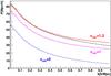 |
Fig. 1 1D power spectrum (P1D) for our simulation with cHR = 0 (lower, blue histogram), cHR = 1 (magenta) and cHR = 1.2 (upper, red), where cHR is defined in Eq. (2), compared to expectation from Eq. (1) (black continuous line). |
The matter density, in pixels located along the line of sight of each quasar, was evolved to the redshift of the pixel by multiplying δρ/ρ by D(z) at the redshift of the considered pixel. This provided us with density spectra in 3.2 Mpc/h bins. We did not interpolate to regular bins, e.g. in log (λ), and then interpolate back to regular bins in Mpc to compute the power spectrum. Since we did average the flux over (12.8 Mpc/h)3 pixels before applying an FFT to compute the power spectrum (Sect. 3.1), we believe this is a minor effect.
Because QSOs sample only a very small transverse region, such a simulation misses a significant contribution to the power spectrum coming from transverse scales smaller than the 3.2 Mpc/h pixel size. This is very clear for the 1D power spectrum, which is an integral of the 3D power spectrum over k ⊥ (Kaiser & Peacock 1991) and therefore includes large k ⊥ :  (1)This missing small-scale contribution is illustrated in Fig. 1, where the 1D power spectrum of the matter density for the simulation with 3.2 Mpc/h pixels (lower blue histogram, CHR = 0) appears significantly lower than the expectation from Eq. (1). To compensate for the missing contribution, we have generated 20 high-resolution (HR) GRF simulations with a volume corresponding to one pixel of our large-volume, low-resolution simulations (LR), i.e. (3.2 Mpc/h)3, and a pixel size of 200 kpc/h. When simulating the matter density along a quasar line-of-sight, for each large pixel we randomly selected one of the HR simulations, and we defined the density in the small pixels as
  (2)As illustrated in Fig. 1, if we just add the LR and HR simulations (i.e. cHR = 1 in Eq. (2)) the 1D power spectrum of the matter density is still slightly smaller than predicted by Eq. (1)1. This is not surprising since we do not have any correlation between the HR simulations in neighboring large pixels. Using an effective correction factor cHR = 1.2 results in a P1D(k), which fits Eq. (1) well, at least in the k ∥ range relevant for BAO, see Fig. 1.
McDonald & Eisenstein (2007) show that the observed power spectrum, Pobs(k), is the sum of the true power spectrum, a sampling contribution and a noise contribution:  (3)where, in the absence of pixel weighting,
  is the inverse of the surface density of quasars (in Mpc-2). Equation (3) indicates that the accurate description achieved for P1D at k ∥ ≤ 0.3, ensures a good description of Pobs(k) in the range relevant to BAO.
The next step was to go from the matter density fluctuations, to QSO transmitted flux fractions F = exp( − τ), where τ is the optical depth. We use the traditional notation, F, for the transmitted flux fraction, and φ for the QSO flux. We used the relation ![Mathematical equation: \begin{equation} \label{Eq:FGPA} F =\exp \left[- a(z) \exp b \frac{\delta \rho}{\rho} \right]\cdot \end{equation}](/articles/aa/full_html/2011/10/aa17736-11/aa17736-11-eq76.png) (4)This means the lognormal approach was used to get the baryon density from our Gaussian fields (Bi & Davidsen 1997) and the baryon density was transformed into transmitted flux fractions F using the fluctuating Gunn-Peterson approximation (Croft et al. 1998; Gnedin & Hui 1998).
(4)This means the lognormal approach was used to get the baryon density from our Gaussian fields (Bi & Davidsen 1997) and the baryon density was transformed into transmitted flux fractions F using the fluctuating Gunn-Peterson approximation (Croft et al. 1998; Gnedin & Hui 1998).
We followed the procedure of McDonald (2003) to take the effect of the peculiar velocities into account: we accounted for the expansion or contraction of cells by translating each cell edge in real space into redshift space using the average velocity of the two cells that the edge separates. The optical depth contributed by each real-space cell was then distributed to multiple redshift-space pixels based on its fractional overlap with each.
The value of b in Eq. (4) was fixed to b = 2 − 0.7(γ − 1) = 1.58 for an equation of state parameter γ = 1.6 (Hui & Gnedin 1997). The value of a(z) was fitted to reproduce the experimental 1D power spectrum and the resulting mean transmitted flux fraction  was checked to be in good agreement with the data, as illustrated by Fig. 2. We could alternatively have fitted and checked P1D. More precisely, McDonald et al. (2006) measure P1D for k ∥ between ≈ 0.14 and ≈ 1.8 h/Mpc and 2.2 < z < 4.2, and in each bin in z we fixed a(z) to fit the first four bins in k, from ≈0.14 to ≈0.28 h/Mpc. We did not fit higher k bins because our simulations do not include nonlinear effects and are not expected to fit data at high k. It would have been more natural to use 100 kpc/h pixel size for the HR simulations, a typical value of the Jeans scale. In this case one only needs a correction factor cHR = 1.12, but one cannot simultaneously reproduce and P1D.
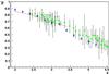 |
Fig. 2 Mean transmitted flux fraction, |
Peculiar velocities introduce a dependence on μ = k ∥ /k in the redshift-space power spectrum: on large scales we have P(k,μ) = (1 + βμ2)2P0(k), where P0(k) is the isotropic real-space power spectrum (Kaiser 1987). For galaxy surveys, β is related to the bias and the growth rate of structure, but for Ly-α forest it is an independent parameter (McDonald et al. 2000). Figure 3 shows the ratio of the power spectra in redshift-space to that in real-space for our simulation2. This ratio follows Kaiser formula in the k range relevant to BAO, k < 0.2. The departure at higher k is because our implementation of velocities is only valid for scales larger than a few (3.2 Mpc/h) pixels. The ratio of power spectra is unity in the transverse direction (μ = 0) and about five in the longitudinal direction (μ = 1), which corresponds to β = 1.2 in Kaiser formula. This is to be compared to β = 1.58 according to McDonald (2003) simulations and 0.38 < β < 1.05, as measured with first BOSS data (Slosar et al. 2011). However, the value of β obtained by BOSS is contaminated by the presence of damped Ly-α systems and metal lines in the quasar spectra. We also observe a bias b = 0.19 relative to the matter power spectrum, to be compared to the 0.17 < b < 0.25 measured with BOSS data.
To get the flux, φi(λ), of quasar i, the transmitted flux fraction, Fi(λ), must be multiplied by the quasar’s unabsorbed spectrum, i.e. the quasar spectrum, including the QSO emission lines, if there were no absorption. The principal component analysis (PCA) of Suzuki et al. (2005) was used to generate a random PCA unabsorbed spectrum for each mock spectrum, which was normalized according to the g-band magnitude of the quasar. Noise was added according to the characteristics of the BOSS spectrograph, including readout noise, sky noise, and signal noise and assuming four exposures of 900 s, for each QSO spectrum. Figure 4 presents the mean signal-to-noise ratio per 1 Å bin in the Ly-α forest, which varies from 14 for a quasar magnitude mg = 19 to 1.6 for mg = 22. Figure 5 shows an example of such a mock spectrum. The pdf of the transmitted flux fraction is presented in Fig. 6. For high-resolution bins, this pdf exhibits peaks at zero and unity, but for low resolutions bins, the flux is averaged and there is a single peak around  . In addition, due to noise the transmitted flux fraction can be larger than unity and also negative.
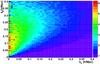 |
Fig. 3 2D power spectrum P(k ⊥ ,k ∥ ) in redshift space divided by the 2D power spectrum in real space. |
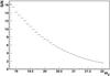 |
Fig. 4 Mean signal-to-noise ratio in the Ly-α forest for 1Å bins, as a function of the quasar magnitude in the g band. |
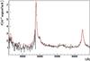 |
Fig. 5 Mock spectrum of a quasar with redshift z = 3.02 and magnitude mg = 21.30. The continuous red line is the input PCA unabsorbed spectrum. |
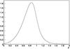 |
Fig. 6 Probability distribution function of the transmitted flux fraction in the 3.8 Mpc/h simulation bins. |
3. From spectra to BAO signal
The mock spectra, produced as described above, were analyzed to reconstruct the power spectrum and the BAO scale.
3.1. Power spectrum estimator
The flux φi in mock spectrum i must be divided by the product of  and the quasar’s unabsorbed spectrum ci in order to provide the fluctuation of the transmitted flux fraction, δF(λ), as
 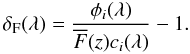 (5)This requires estimates of and ci(λ). In Sect. 4.2 we discuss various methods of doing this. In this section we use the true values of and ci, a procedure that only slightly overestimates the precision of the determination of the BAO signal. A grid with (12.8 Mpc/h)3 cells was filled with the part of the δF spectra that corresponds to the Ly-α forest; we selected 1041 < λ < 1181 Å, in the quasar rest frame. An unweighted average of δF was calculated for all pixels of all Ly-α forest spectra lying in a considered grid cell. Some grid cells do not contain any Ly-α forest spectra. The average of all other cells was computed and this average subtracted from the content of all filled cells, while the content of unfilled cells remained zero. This was done in order to avoid including the Fourier transform of the quasar spatial distribution in the power spectrum. This is analogous to subtracting a synthetic catalog in the case of galaxy surveys, as advocated by Feldman et al. (1994).
A Fourier transform of the resulting grid was performed and the modulus squared computed for each mode (kx,ky,kz), which gives the power for the considered mode. The angular-averaged power spectrum was then obtained as the average of the power for all the modes with | k | in a given bin; however, we did not include purely radial (0,0,kz) and purely transverse (kx,ky,0) modes. The former correspond to Fourier transforms along quasar lines of sight. These are severely affected by the uncertainty on the quasar’s unabsorbed spectrum estimate. The latter have a very large sampling term contribution owing to the high value of  . Purely transverse modes are 5.8% of all modes at the first BAO peak and 3.4% at the second BAO peak, while the number of purely longitudinal modes is less than 0.01% of all modes at the first BAO peak. The error on P(k) is obtained as the rms of the power in all modes in the considered k bin, divided by the square root of the number of modes. The correlations between the power in different k bins are expected to be weak and we neglect them.
The resulting power spectrum exceeds Eq. (3) by about 10%, as illustrated in Fig. 7. We see that the sampling and noise contributions are of similar sizes and much larger than the input (LSS) power spectrum, which means that the BAO oscillations will be considerably diluted, as can be seen in Fig. 8.
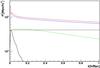 |
Fig. 7 Power spectrum in the simulation (red upper histogram) compared to the expectation of Eq. (3) (blue, just below red). The latter is the sum of the input power spectrum (black, decreasing quickly with k), the noise contribution (black, constant with k), and the sampling contribution (green, decreasing slowly with k). |
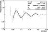 |
Fig. 8 Power spectrum for a realization of the nominal setup (15 QSO/deg2) divided by a 7th order polynomial and fitted with Blake & Glazebrook (2003) formula, see text. |
3.2. Reconstruction of the BAO scale
To infer the BAO scale, the angular-averaged power spectrum was first fitted by a polynomial. The power spectrum divided by this polynomial was then fitted with ![Mathematical equation: \begin{equation} \label{Eq:fit1D} 1+ A \left \{ k \exp \left[\left(\frac{-k}{\tau}\right)^p \right] \sin\left[2\pi \frac{k}{k_A} \;\right] \right\}, \end{equation}](/articles/aa/full_html/2011/10/aa17736-11/aa17736-11-eq126.png) (6)as suggested by Blake & Glazebrook (2003). This provides the (isotropic) BAO scale kA, as illustrated in Fig. 8. This figure corresponds to an average realization with Δχ2 = 16.8 and the BAO oscillations are quite visible. Their amplitude is less than a percent, which means they are considerably diluted relative to the input power spectrum where they are on the order of 10%. This is due to the sampling and noise contributions to the observed power spectrum, see Eq. (3).
(6)as suggested by Blake & Glazebrook (2003). This provides the (isotropic) BAO scale kA, as illustrated in Fig. 8. This figure corresponds to an average realization with Δχ2 = 16.8 and the BAO oscillations are quite visible. Their amplitude is less than a percent, which means they are considerably diluted relative to the input power spectrum where they are on the order of 10%. This is due to the sampling and noise contributions to the observed power spectrum, see Eq. (3).
The upper limit of the polynomial fit range was set to 0.24, due to our 12.8 Mpc/h FFT cells, which result in a maximum k of 0.245 h/Mpc in x, y or z direction. The lower limit and the order of the polynomial were set so as to get a good χ2 to the power spectrum obtained for some additional simulations that did not include the BAO features. These simulations were generated using the power spectrum with baryons but without BAO by Eisenstein & Hu (1998). We noted that using a polynomial of too low a degree could result in a significant bias in the reconstructed BAO scale, while on the other hand increasing the polynomial degree beyond what is needed to get a good fit could degrade the performance (i.e. increase the rms of kA) because the polynomial starts to fit the BAO features. Depending on the studied scenario, the lower limit was set between 0.02 and 0.05 h/Mpc, and the order of the polynomial was either six or seven. The range for oscillation fitting was set to 0.05 < k < 0.2 h/Mpc. This range is somewhat narrower, which avoids edge effects in the polynomial fit, and also high k values for which nonlinear effects are important.
Ten GRF simulations were produced. Each of them was used ten times, with different random seeds to generate the quasar positions. One hundred values of kA were then obtained, and their rms provides an estimate of the statistical precision on the BAO scale. This was done for several different scenarios, and the results are presented in Sect. 4.1. The mean value of the error on kA returned by the Minuit fitting package (James & Roos 1975) is found to be compatible with the rms of kA, which confirms that our estimate of the error on P(k) and our neglect of correlations are both reasonable.
3.2.1. Radial and transverse BAO scales
In addition to the anisotropy of P(k) due to peculiar velocities, the reconstructed power spectrum, Pobs(k), involves a stronger anisotropy due to the sampling contribution in Eq. (3), which depends on k ∥ . It is difficult to find a functional form to fit the 2D power spectrum P(k ⊥ ,k ∥ ). Instead, P(k ⊥ ,k ∥ ) was divided by the polynomial obtained from the 1D fit (previous section) to provide a “reduced” power spectrum, which was then smoothed using algorithms implemented in the CERN ROOT package. The ratio of the reduced power spectrum to the smoothed reduced power spectrum was fitted with ![Mathematical equation: \begin{equation} \label{Eq:fit2D} 1+ A \left \{ k \exp \left[\left(\frac{-k}{\tau}\right)^p \right] \sin\left[2\pi \sqrt{\frac{k_\perp}{k^A_\perp} +\frac{k_\parallel}{k^A_\parallel}}\;\right] \right\}. \end{equation}](/articles/aa/full_html/2011/10/aa17736-11/aa17736-11-eq132.png) (7)The rms from the 100 resulting values of
(7)The rms from the 100 resulting values of  and
and  provides an estimate of the error on the transverse and radial BAO scales. However, this 2D fitting is quite delicate. It does not work in all cases and a more sophisticated procedure would be needed to analyze real data.
4. Results
4.1. Results with the true quasar’s unabsorbed spectrum
In this section we discuss the performance of BAO reconstruction in the ideal case where in Eq. (5) we divided by the true and ci(λ). By default the simulation was performed for 15 QSO/deg2 in the redshift range 2.2 < z < 3.5 and with magnitude 18 < mg < 22. The results were slightly scaled to correspond to the 10 000 deg2 of the BOSS survey. Different scenarios in terms e.g. of number of quasars per deg2 or noise level were studied. Table 1 presents, for each scenario, the rms in percent for the isotropic (kA), radial (k ∥ ), and transverse (k ⊥ ) BAO scales. With 100 simulations, the statistical error on the rms, is just rms rms, e.g. 0.16, 0.40 and 0.28% for the nominal case (line 4). To assess the significance of the BAO detection, we also give the difference of χ2 relative to the case with no BAO (A = 0 in Eq. (6)).
Rms of the BAO scale and significance of BAO feature detection, for different scenarios.
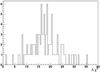 |
Fig. 9 Nominal simulation (15 QSO/deg2). Difference between the χ2 for the nominal fit (Eq. (6)) and the χ2 for no oscillations (A = 0 in Eq. (6)) for the 100 realizations. |
We start without noise and with vanishing velocity field (Table 1, line 1). In this case, the transverse scale is much better reconstructed than the radial one because there are more transverse than radial modes (two transverse directions and only one radial). Including peculiar velocities amplifies the power spectrum in the radial direction and dramatically improves the radial scale reconstruction, as can be seen on line 2.
The nominal case is obtained when we add noise according to the BOSS setup, which results in rms of 2.28 ± 0.16, 6.79 ± 0.48, and 3.86 ± 0.27 percent for the isotropic, transverse, and radial BAO scales, respectively (line 4 of Table 1). On average over the 100 simulations, Δχ2 is 17.4, which means a significant detection of BAO features. This is, however, just an average, and the difference of χ2 ranges from 2 to 35, as illustrated by Fig. 9. At this point, we note that the (2Gpc/h)3 Horizon simulation has a 17 times smaller angular coverage than our simulation. The χ2 differences for the Horizon simulation would therefore be typically one for the BOSS Ly-α survey, so, as announced in Sect. 2.1, the Horizon simulation is clearly not large enough to study the reconstruction of the BAO features with BOSS survey.
For the same nominal setup, an updated version (McDonald, priv. comm.) of the analytic estimate of McDonald & Eisenstein (2007) gives an error of 1.8% on the isotropic BAO scale when weighting pixels according to signal-to-noise ratio. Without weighting the computed error increases to 1.91%. Our result, 2.28 ± 0.16, is larger by a factor 1.19 ± 0.08, which is consistent with the fact that we find a power spectrum that is about 10% larger than predicted by formula (3), as illustrated in Fig. 7. Greig et al. (2011) very recently published simulation results; they get an error of 1.38% on the BAO scale for a fixed S/N = 5, whereas we have in average S/N = 3.1. When we decrease S/N by a factor 1.7, we observe an increase in the rms by a factor 1.75, so it is reasonable that an increase of S/N by a factor 5/3.1 = 1.6, reduces the rms by a factor 2.28/1.38 = 1.65.
Comparison of lines 3, 4, and 5 in Table 1 illustrates the variations in the performance with the quasar density. The sampling and noise contributions to the power spectrum (Eq. (1)) scale as 1/NQSO. If we could completely neglect PF(k) in Eq. (1), we would therefore expect the rms of the BAO to scale as 1/NQSO. We observe a decrease in the rms with the quasar density, which is not as strong as 1/NQSO but statistically compatible with the  dependence found by Greig et al. (2011). We investigated the dependence on the noise level. Line 6 shows that increasing the noise by a factor 1.7 results in a significant degradation of the performance. As is clear from Fig. 7, increasing the noise power spectrum by a factor 1.72 makes it the dominant contribution to the total power spectrum.
We also considered the case of the BigBOSS project, assuming 60 QSO/deg2 up to a g-magnitude of 23, over 14 000 deg2 (last line of Table. 1). With a 4-m telescope and five exposures of 900 s instead of a 2.5-m telescope and five exposures, the noise is reduced by nearly a factor two relative to BOSS case. The resulting rms of the BAO scale is improved by a factor 4.2 relative to BOSS nominal case.
Finally, we note that naively combining the rms on the transverse and radial scales in Table 1 results in an error that is significantly larger than the rms on the isotropic scale. This is (partly) due to a significant anticorrelation between the reconstructed transverse and radial scales. When the rms is quite small, e.g. in the nominal case with 20 QSO/deg2 or in the BigBOSS case, taking a correlation coefficient of typically − 0.40 into account, results in a combined rms, in agreement with the rms on the isotropic case. In other cases, the combined rms is still larger by a factor on the order of 1.2, up to a factor 1.4 for the case without velocities. This confirms that fitting the BAO features in 2D is difficult, in particular when the quasar density is low.
4.2. Effect of unabsorbed spectrum error
Using Eq. (5) to obtain δF requires an estimate of  for each spectrum and the above results were obtained using the true value of this product. One can get a fair estimate of
  from the observed spectra, up to a normalization factor that is completely degenerate with the normalization of the ci. On the other hand, with the resolution and the S/N of the BOSS survey, the unabsorbed spectra, ci(λ), cannot be accurately determined from the observed spectra (see Fig. 5). A possible approach is to fit a power law in λ on the red side of the Ly-α emission line, to extrapolate it in the Ly-α forest, possibly multiplying it by some average shape of the unabsorbed spectrum as a function of λrf, the quasar rest-frame wavelength (e.g., Slosar et al. 2011). We could not do that because our mocks are based on PCA by Suzuki et al. (2005), which only extend up to 1600 Å in the quasar rest frame and therefore do not allow for a reliable power law fit. Reliable fits will be possible with the PCA provided very recently by Pâris et al. (2011), extending up to 2000 Å.
Instead, we computed the average spectrum in the forest, as a function of λrf. Then we divided each spectrum by this average spectrum, fitted the result with a power law in λ, and finally divided by this power law. This is dividing the mock spectrum by an estimate of . For the nominal setup, this results in an rms of (2.55 ± 0.16)% for the BAO scale, only a factor 1.12 ± 0.04 larger than what is obtained with the true unabsorbed spectrum. We also note that, while we did not observe any bias on the reconstructed BAO scale when using the true unabsorbed spectrum, with this approximate unabsorbed spectrum, there is a bias of − 0.59 ± 0.18%, which is, however, much smaller than the 2.55% statistical error on the BAO scale. In this procedure, since we do a power law fit along the quasar spectra, we remove large scale power in the radial direction, so all modes with a low value of k ∥ are strongly reduced and P(k) becomes very anisotropic. In this case, the smoothing used in the 2D fit procedure does not make sense, so we do not get results for the transverse and radial BAO scales, separately. A more sophisticated procedure would need to be developed.
Another possible approach is to use PCA to predict the unabsorbed spectrum in the forest from the flux redward of the Ly-α emission line. However, we cannot use mock spectra generated with PCA to study how precisely PCA reconstruct the unabsorbed spectrum. Instead we used 78 observed unabsorbed spectra, cobs(λ), and their corresponding PCA estimates, cPCA(λ) provided by Pâris et al. (2011). The observed unabsorbed spectra were manually estimated from high S/N SDSS II spectra, while the PCA unabsorbed spectra were obtained for each spectrum by a PCA analysis of the 77 other spectra. For each of our spectra, with true unabsorbed spectrum ci(λ), we randomly selected spectrum j within the 78 spectra from Pâris et al. (2011), and used 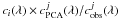 as an unabsorbed spectrum. Since there is much less uncertainty on we used the true value of this function. This results in an rms of (2.73 ± 0.19)% for the BAO scale, i.e. a factor 1.20 ± 0.11 larger than what is obtained when using the true unabsorbed spectrum, and the bias is + 0.45 ± 0.20%. In addition, most of the unabsorbed spectrum estimates of Pâris et al. (2011) are quite good while a few are grossly wrong. Therefore a significant improvement is to be expected if a criteria can be found to identify a-priori the spectra for which PCA will fail so that a different approach can be used for these few spectra. Finally, the PCA unabsorbed spectrum estimates of Pâris et al. (2011) were obtained for high S/N spectra, but PCA estimates might not be very sensitive to additional noise.
5. Constraint on cosmological parameters
The observation of the transverse and radial BAO scales provides a measurement of dT(z)/s and dH(z)/s, respectively, where dT(z) is the comoving angular distance, dH(z) the Hubble distance and s the sonic horizon at decoupling. For a flat ΛCDM universe dT and dH are 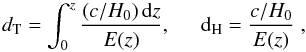 (8)where
 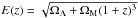 .
.
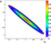 |
Fig. 10 Confidence level contours in the (w0,wa) parameter plane for Planck + BOSS LRG + BOSS Ly-α. |
To estimate the sensitivity to parameters describing the dark energy equation of state, p = wρ, we follow the procedure explained in Blake & Glazebrook (2003). We introduce the z dependence of w as w(z) = w0 + wa·z/(1 + z) and replace ΩΛ in E(z) in Eq. (8) by ![Mathematical equation: \begin{equation} \Omega_\Lambda \longrightarrow \Omega_{\Lambda} \exp \left[ 3 \int_0^z \frac{1+w(z^\prime)}{1+z^\prime } {\rm d}z^\prime \right].\vspace{-1.5mm} \end{equation}](/articles/aa/full_html/2011/10/aa17736-11/aa17736-11-eq184.png) (9)Using the relative errors on the transverse (6.79%) and radial (3.86%) BAO scales, obtained for the nominal setup (Table 1, line 4), and taking the anticorrelation into account, we can compute the Fisher matrix for the five cosmological parameters Ωm, Ωb, h, w0, and wa. We also use the Fisher matrix for Planck mission computed for the Euclid proposal (Laureijs 2009), which assumes a flat universe and involves the eight parameters: Ωm, Ωb, h, w0, wa, σ8, ns (spectral index of the primordial power spectrum), and τ (optical depth to the last-scatter surface). Combining BOSS and Planck Fisher matrices allows us to compute the errors on dark energy parameters. If we define the factor of merit as the inverse of the 1-σ uncertainty ellipse in the (w0,wa) plane, we get 34 for Planck and BOSS LRG survey. When we add BOSS Ly-α survey, this increases to 48. The corresponding confidence level contours are plotted in Fig. 10.
(9)Using the relative errors on the transverse (6.79%) and radial (3.86%) BAO scales, obtained for the nominal setup (Table 1, line 4), and taking the anticorrelation into account, we can compute the Fisher matrix for the five cosmological parameters Ωm, Ωb, h, w0, and wa. We also use the Fisher matrix for Planck mission computed for the Euclid proposal (Laureijs 2009), which assumes a flat universe and involves the eight parameters: Ωm, Ωb, h, w0, wa, σ8, ns (spectral index of the primordial power spectrum), and τ (optical depth to the last-scatter surface). Combining BOSS and Planck Fisher matrices allows us to compute the errors on dark energy parameters. If we define the factor of merit as the inverse of the 1-σ uncertainty ellipse in the (w0,wa) plane, we get 34 for Planck and BOSS LRG survey. When we add BOSS Ly-α survey, this increases to 48. The corresponding confidence level contours are plotted in Fig. 10.
6. Summary and conclusion
In this paper we have investigated the possibility of constraining the BAO scale from the quasar Ly-α forest and in particular the precision that will be reached by any survey such as BOSS. To this aim, we simulated realistic mock quasar spectra mimicking the survey. Because the volume of the largest N-body simulations is too small for such a study, we resorted to GRFs, combined with lognormal approximation and FGPA. We investigate the effect of noise, peculiar velocity, and random quasars’ unabsorbed spectra generated using a principal component analysis (PCA).
The power spectrum of the transmitted flux fraction in the Ly-α forest was thus computed and was either fitted in 2D to reconstruct the radial and transverse BAO scales, or averaged over angles and fitted in 1D to reconstruct the isotropic BAO scale. This was done over 100 realizations, resulting in an rms of 2.3% on the isotropic BAO scale, or 6.8% and 3.9% on the transverse and radial BAO scales determinations separately. This is compatible with analytical estimates by McDonald & Eisenstein (2007). The BAO features are detected with an average Δχ2 of 17, and the FOM for dark energy parameter determination improves from 34 for Planck and BOSS LRG survey to 48 when the Ly-α survey constraint is included. We note, however, that Δχ2 varies significantly between realizations, ranging from 2 to 35.
These above estimates were obtained assuming a perfect knowledge of the quasar’s unabsorbed spectrum. Errors on the estimate of the unabsorbed spectrum will increase the errors on the BAO scale by 10 to 20% and result in subpercent biases, overall quite small compared to the statistical error. The effect of the presence of damped Ly-α and metal lines on the BAO measurement was not included in our mock spectra.
In Eq. (1) we integrated up to /(100 kpc/), which corresponds to a typical value of the Jeans’ scale. This however is only a reduction of a few percent relative to the integral up to infinity.
The power spectra were obtained without noise and using all pixels of the box, not just those along some random QSO lines. This removes the contribution from the noise and sampling terms so that , see Eq. (3).
Acknowledgments
We would like to thank Rupert Croft, Andreu Font-Ribera, Patrick McDonald, and Anze Slosar for useful discussions and the last two for comments to the paper.
References
- Aracil, B., Petitjean, P., Pichon, C., & Bergeron, J. 2004, A&A, 419, 811 [NASA ADS] [CrossRef] [EDP Sciences] [Google Scholar]
- Bashinsky, S., & Bertschinger, E. 2002, Phys. Rev. D, 65, 123008 [NASA ADS] [CrossRef] [Google Scholar]
- Becker, G. D., Rauch, M., & Sargent, W. L. W. 2007, ApJ, 662, 72 [NASA ADS] [CrossRef] [Google Scholar]
- Bi, H., & Davidsen, A. F. 1997, ApJ, 479, 523 [NASA ADS] [CrossRef] [Google Scholar]
- Bi, H. G., Boerner, G., & Chu, Y. 1992, A&A, 266, 1 [NASA ADS] [Google Scholar]
- Blake, C., & Glazebrook, K. 2003, ApJ, 594, 665 [NASA ADS] [CrossRef] [Google Scholar]
- Bolton, J. S., Haehnelt, M. G., Viel, M., & Springel, V. 2005, MNRAS, 357, 1178 [NASA ADS] [CrossRef] [Google Scholar]
- Bovy, J., Hennawi, J. F., Hogg, D. W., et al. 2011, ApJ, 729, 141 [NASA ADS] [CrossRef] [Google Scholar]
- Cen, R., Miralda-Escudé, J., Ostriker, J. P., & Rauch, M. 1994, ApJ, 437, L9 [Google Scholar]
- Cole, S., Percival, W. J., Peacock, J. A., et al. 2005, MNRAS, 362, 505 [NASA ADS] [CrossRef] [Google Scholar]
- Coppolani, F., Petitjean, P., Stoehr, F., et al. 2006, MNRAS, 370, 1804 [NASA ADS] [CrossRef] [Google Scholar]
- Cowie, L. L., Songaila, A., Kim, T.-S., & Hu, E. M. 1995, AJ, 109, 1522 [NASA ADS] [CrossRef] [Google Scholar]
- Croft, R. A. C., Weinberg, D. H., Katz, N., & Hernquist, L. 1998, ApJ, 495, 44 [NASA ADS] [CrossRef] [Google Scholar]
- Croft, R. A. C., Weinberg, D. H., Pettini, M., Hernquist, L., & Katz, N. 1999, ApJ, 520, 1 [NASA ADS] [CrossRef] [Google Scholar]
- Eisenstein, D. J., & Hu, W. 1998, ApJ, 496, 605 [NASA ADS] [CrossRef] [Google Scholar]
- Eisenstein, D. J., Zehavi, I., Hogg, D. W., et al. 2005, ApJ, 633, 560 [NASA ADS] [CrossRef] [Google Scholar]
- Eisenstein, D. J., Weinberg, D. H., Agol, E., et al. 2011, AJ, 142, 72 [Google Scholar]
- Fan, X., Carilli, C. L., & Keating, B. 2006, ARA&A, 44, 415 [NASA ADS] [CrossRef] [Google Scholar]
- Faucher-Giguère, C.-A., Prochaska, J. X., Lidz, A., Hernquist, L., & Zaldarriaga, M. 2008, ApJ, 681, 831 [NASA ADS] [CrossRef] [Google Scholar]
- Feldman, H. A., Kaiser, N., & Peacock, J. A. 1994, ApJ, 426, 23 [NASA ADS] [CrossRef] [Google Scholar]
- Fukugita, M., Hogan, C. J., & Peebles, P. J. E. 1998, ApJ, 503, 518 [NASA ADS] [CrossRef] [Google Scholar]
- Gnedin, N. Y., & Hui, L. 1998, MNRAS, 296, 44 [NASA ADS] [CrossRef] [Google Scholar]
- Greig, B., Bolton, J. S., & Wyithe, J. S. B. 2011, MNRAS, in press [arXiv:1105.4747] [Google Scholar]
- Guimarães, R., Petitjean, P., Rollinde, E., et al. 2007, MNRAS, 377, 657 [NASA ADS] [CrossRef] [Google Scholar]
- Gunn, J. E., & Peterson, B. A. 1965, ApJ, 142, 1633 [NASA ADS] [CrossRef] [Google Scholar]
- Hui, L., & Gnedin, N. Y. 1997, MNRAS, 292, 27 [Google Scholar]
- Hui, L., & Haiman, Z. 2003, ApJ, 596, 9 [NASA ADS] [CrossRef] [Google Scholar]
- James, F., & Roos, M. 1975, Comput. Phys. Commun., 10, 343 [NASA ADS] [CrossRef] [PubMed] [Google Scholar]
- Jiang, L., Fan, X., Cool, R. J., et al. 2006, AJ, 131, 2788 [NASA ADS] [CrossRef] [Google Scholar]
- Kaiser, N. 1987, MNRAS, 227, 1 [NASA ADS] [CrossRef] [Google Scholar]
- Kaiser, N., & Peacock, J. A. 1991, ApJ, 379, 482 [NASA ADS] [CrossRef] [Google Scholar]
- Kim, Y.-R., & Croft, R. A. C. 2008, MNRAS, 387, 377 [NASA ADS] [CrossRef] [Google Scholar]
- Kirkpatrick, J. A., Schlegel, D. J., Ross, N. P., et al. 2011, ApJ, accepted [arXiv:1104.4995] [Google Scholar]
- Komatsu, E., Dunkley, J., Nolta, M. R., et al. 2009, ApJS, 180, 330 [NASA ADS] [CrossRef] [Google Scholar]
- Laureijs, R. 2009 [arXiv:0912.0914] [Google Scholar]
- McDonald, P., & Miralda-Escudé, J. 1999, ApJ, 518, 24 [NASA ADS] [CrossRef] [Google Scholar]
- McDonald, P. 2003, ApJ, 585, 34 [NASA ADS] [CrossRef] [Google Scholar]
- McDonald, P., & Eisenstein, D. J. 2007, Phys. Rev. D, 76, 063009 [NASA ADS] [CrossRef] [Google Scholar]
- McDonald, P., Miralda-Escudé, J., Rauch, M., et al. 2000, ApJ, 543, 1 [NASA ADS] [CrossRef] [Google Scholar]
- McDonald, P., Miralda-Escudé, J., Rauch, M., et al. 2001, ApJ, 562, 52 [NASA ADS] [CrossRef] [Google Scholar]
- McDonald, P., Seljak, U., Cen, R., Bode, P., & Ostriker, J. P. 2005, MNRAS, 360, 1471 [NASA ADS] [CrossRef] [Google Scholar]
- McDonald, P., Seljak, U., & Burles, e. a. 2006, ApJS, 163, 80 [NASA ADS] [CrossRef] [Google Scholar]
- McQuinn, M., & White, M. 2011, MNRAS, 727 [Google Scholar]
- Meiksin, A., White, M., & Peacock, J. A. 1999, MNRAS, 304, 851 [NASA ADS] [CrossRef] [Google Scholar]
- Miralda-Escudé, J., Cen, R., Ostriker, J. P., & Rauch, M. 1996, ApJ, 471, 582 [NASA ADS] [CrossRef] [Google Scholar]
- Padmanabhan, N., & White, M. 2009, Phys. Rev. D, 80, 063508 [Google Scholar]
- Page, L., Nolta, M. R., Barnes, C., et al. 2003, ApJS, 148, 233 [NASA ADS] [CrossRef] [Google Scholar]
- Palanque-Delabrouille, N., Yeche, C., Myers, A. D., et al. 2011, A&A, 530, A122 [NASA ADS] [CrossRef] [EDP Sciences] [Google Scholar]
- Pâris, I., Petitjean, P., Rollinde, E., et al. 2011, A&A, 530, A50 [NASA ADS] [CrossRef] [EDP Sciences] [Google Scholar]
- Peebles, P. J. E., & Yu, J. T. 1970, ApJ, 162, 815 [NASA ADS] [CrossRef] [Google Scholar]
- Percival, W. J., Reid, B. A., Eisenstein, D. J., et al. 2010, MNRAS, 401, 2148 [NASA ADS] [CrossRef] [Google Scholar]
- Petitjean, P., Webb, J. K., Rauch, M., Carswell, R. F., & Lanzetta, K. 1993, MNRAS, 262, 499 [NASA ADS] [CrossRef] [Google Scholar]
- Petitjean, P., Mueket, J. P., & Kates, R. E. 1995, A&A, 295, L9 [NASA ADS] [Google Scholar]
- Prunet, S., Pichon, C., Aubert, D., et al. 2008, ApJS, 178, 179 [NASA ADS] [CrossRef] [Google Scholar]
- Rauch, M. 1998, ARA&A, 36, 267 [NASA ADS] [CrossRef] [Google Scholar]
- Rauch, M., Miralda-Escude, J., Sargent, W. L. W., et al. 1997, ApJ, 489, 7 [NASA ADS] [CrossRef] [Google Scholar]
- Ricotti, M., Gnedin, N. Y., & Shull, J. M. 2000, ApJ, 534, 41 [NASA ADS] [CrossRef] [Google Scholar]
- Rollinde, E., Petitjean, P., Pichon, C., et al. 2003, MNRAS, 341, 1279 [NASA ADS] [CrossRef] [Google Scholar]
- Rollinde, E., Srianand, R., Theuns, T., Petitjean, P., & Chand, H. 2005, MNRAS, 361, 1015 [NASA ADS] [CrossRef] [Google Scholar]
- Ross, N. P., Myers, A. D., Sheldon, E. S., et al. 2011, ApJ, submitted [arXiv:1105.0606] [Google Scholar]
- Schaye, J., Theuns, T., Leonard, A., & Efstathiou, G. 1999, MNRAS, 310, 57 [NASA ADS] [CrossRef] [Google Scholar]
- Schaye, J., Aguirre, A., Kim, T.-S., et al. 2003, ApJ, 596, 768 [NASA ADS] [CrossRef] [Google Scholar]
- Schlegel, D., White, M., & Eisenstein, D. 2009, Astro2010, AGB Stars and Related Phenomenastro2010: The Astronomy and Astrophysics Decadal Survey, 314 [Google Scholar]
- Slosar, A., Ho, S., White, M., & Louis, T. 2009, J. Cosmol. Astro-Part. Phys., 10, 19 [Google Scholar]
- Slosar, A., Font-Ribera, A., Pieri, M. M., et al. 2011, J. Cosmol. Astro-Part. Phys., 09, 001 [Google Scholar]
- Songaila, A. 2004, AJ, 127, 2598 [NASA ADS] [CrossRef] [Google Scholar]
- Sunyaev, R. A., & Zeldovich, Y. B. 1970, Ap&SS, 7, 3 [NASA ADS] [Google Scholar]
- Suzuki, N., Tytler, D., Kirkman, D., O’Meara, J. M., & Lubin, D. 2005, ApJ, 618, 592 [NASA ADS] [CrossRef] [Google Scholar]
- Teyssier, R. 2002, A&A, 385, 337 [NASA ADS] [CrossRef] [EDP Sciences] [Google Scholar]
- Teyssier, R., Pires, S., Prunet, S., et al. 2009, A&A, 497, 335 [NASA ADS] [CrossRef] [EDP Sciences] [Google Scholar]
- Theuns, T., Leonard, A., Efstathiou, G., Pearce, F. R., & Thomas, P. A. 1998, MNRAS, 301, 478 [NASA ADS] [CrossRef] [Google Scholar]
- Theuns, T., Schaye, J., & Haehnelt, M. G. 2000, MNRAS, 315, 600 [NASA ADS] [CrossRef] [Google Scholar]
- Theuns, T., Schaye, J., Zaroubi, S., et al. 2002a, ApJ, 567, L103 [NASA ADS] [CrossRef] [Google Scholar]
- Theuns, T., Viel, M., Kay, S., et al. 2002b, ApJ, 578, L5 [NASA ADS] [CrossRef] [Google Scholar]
- Viel, M., & Haehnelt, M. G. 2006, MNRAS, 365, 231 [NASA ADS] [CrossRef] [Google Scholar]
- Viel, M., Haehnelt, M. G., & Springel, V. 2004, MNRAS, 354, 684 [NASA ADS] [CrossRef] [Google Scholar]
- White, M. 2003, in The Davis Meeting On Cosmic Inflation. 2003 March 22–25, Davis CA., 18 [Google Scholar]
- White, M., Pope, A., Carlson, J., et al. 2009, ArXiv e-prints [Google Scholar]
- Yèche, C., Petitjean, P., Rich, J., et al. 2010, A&A, 523, A14 [NASA ADS] [CrossRef] [EDP Sciences] [Google Scholar]
All Tables
Rms of the BAO scale and significance of BAO feature detection, for different scenarios.
All Figures
|
Fig. 1 1D power spectrum (P1D) for our simulation with cHR = 0 (lower, blue histogram), cHR = 1 (magenta) and cHR = 1.2 (upper, red), where cHR is defined in Eq. (2), compared to expectation from Eq. (1) (black continuous line). |
| In the text | |
|
Fig. 2 Mean transmitted flux fraction, |
| In the text | |
|
Fig. 3 2D power spectrum P(k ⊥ ,k ∥ ) in redshift space divided by the 2D power spectrum in real space. |
| In the text | |
|
Fig. 4 Mean signal-to-noise ratio in the Ly-α forest for 1Å bins, as a function of the quasar magnitude in the g band. |
| In the text | |
|
Fig. 5 Mock spectrum of a quasar with redshift z = 3.02 and magnitude mg = 21.30. The continuous red line is the input PCA unabsorbed spectrum. |
| In the text | |
|
Fig. 6 Probability distribution function of the transmitted flux fraction in the 3.8 Mpc/h simulation bins. |
| In the text | |
|
Fig. 7 Power spectrum in the simulation (red upper histogram) compared to the expectation of Eq. (3) (blue, just below red). The latter is the sum of the input power spectrum (black, decreasing quickly with k), the noise contribution (black, constant with k), and the sampling contribution (green, decreasing slowly with k). |
| In the text | |
|
Fig. 8 Power spectrum for a realization of the nominal setup (15 QSO/deg2) divided by a 7th order polynomial and fitted with Blake & Glazebrook (2003) formula, see text. |
| In the text | |
|
Fig. 9 Nominal simulation (15 QSO/deg2). Difference between the χ2 for the nominal fit (Eq. (6)) and the χ2 for no oscillations (A = 0 in Eq. (6)) for the 100 realizations. |
| In the text | |
|
Fig. 10 Confidence level contours in the (w0,wa) parameter plane for Planck + BOSS LRG + BOSS Ly-α. |
| In the text | |
Current usage metrics show cumulative count of Article Views (full-text article views including HTML views, PDF and ePub downloads, according to the available data) and Abstracts Views on Vision4Press platform.
Data correspond to usage on the plateform after 2015. The current usage metrics is available 48-96 hours after online publication and is updated daily on week days.
Initial download of the metrics may take a while.