| Issue |
A&A
Volume 534, October 2011
|
|
|---|---|---|
| Article Number | A79 | |
| Number of page(s) | 10 | |
| Section | Galactic structure, stellar clusters and populations | |
| DOI | https://doi.org/10.1051/0004-6361/201117626 | |
| Published online | 05 October 2011 | |
Galactic distributions of carbon- and oxygen-rich AGB stars revealed by the AKARI mid-infrared all-sky survey
1
Department of Physics, Nagoya University, Furo-cho, Chikusa-ku, Nagoya, Aichi 464-8602, Japan
2
Department of Astronomy, Graduate School of Science, University of Tokyo, 7-3-1 Hongo, Bunkyo-ku, Tokyo 113-0033, Japan
3
Astronomical Institute, Tohoku University, 6-3 Aramaki, Aoba-ku Sendai 980-8578, Japan
4
UCL-Institute of Origins, Department of Physics and Astronomy, University College London, Gower Street, London WC1E 6BT, UK
5
UCL-Institute of Origins, Mullard Space Science Laboratory, University College London, Holmbury St. Mary, Dorking, Surrey RH5 6NT, UK
6
Kiso Observatory, Institute of Astronomy, University of Tokyo, 10762-30 Mitake, Kiso, Nagano 397-0101, Japan
Received: 4 July 2011
Accepted: 5 August 2011
Abstract
Context. The environmental conditions for asympotic giant branch (AGB) stars to reach the carbon-rich (C-rich) phase are important to understand the evolutionary process of AGB stars. The difference between the spatial distributions of C-rich and oxygen-rich (O-rich) AGB stars is essential for the study of the Galactic structure and the chemical evolution of the interstellar medium.
Aims. We quantitatively investigate the spatial distributions of C-rich and O-rich AGB stars in our Galaxy. We discuss the difference between them and its origin.
Methods. We classify a large number of AGB stars newly detected by the AKARI mid-infrared all-sky survey. In the color–color diagrams, we define their occupation zones based on the locations of known objects. We then obtain the spatial distributions of C-rich and O-rich AGB stars, assuming that they have the same luminosity for a given mass-loss rate.
Results. We find that O-rich AGB stars are concentrated toward the Galactic center and that the density decreases with Galactocentric distance, whereas C-rich AGB stars show a relatively uniform distribution within about 8 kpc of Sun.
Conclusions. Our result confirms the trends reported in previous studies and extends them to a Galactic scale. We discuss the relations between our result, the Galactic metallicity gradient, and the chemical evolution of the ISM in our Galaxy.
Key words: stars: AGB and post-AGB / infrared: ISM / stars: mass-loss / infrared: stars / Galaxy: structure
© ESO, 2011
1. Introduction
Asymptotic giant branch (AGB) stars are low- to intermediate-mass (1–8 M⊙) stars at their final evolutionary stages that undergo mass-loss (e.g. Habing et al. 1985). Their ages range from 0.1 to several Gyr, depending on their initial masses. The spatial distribution of AGB stars roughly traces past star-formation activities.
The AGB stars are divided into three classes based on their carbon-to-oxygen elemental abundance ratios: carbon-rich AGB stars (C-rich; C/O > 1), oxygen-rich AGB stars (O-rich; C/O < 1), and S stars (C/O ~ 1). Many AGB stars in the Milky Way are O-rich (e.g. Habing et al. 1985) and show silicate-dominated circumstellar features. In contrast, some fraction of intermediate-mass AGB stars (1.1–4 M⊙) become C-rich, displaying the features of both carbon-bearing molecules (e.g. C2, CN, HCN, C2H2, and CO) and carbonaceous dust (e.g. amorphous carbon and graphite). This chemical change is triggered when carbon atoms, which are synthesized in the stellar core, are dredged up to the surface by the deep convective envelope.
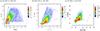 |
Fig. 1 Color–color diagrams in density maps for the AKARI/MIR sources that have 2MASS measurements: a) [J] − [K] versus [K] − [9] , b) [K] − [9] versus [9] − [18] , and c) [J] − [K] versus [9] − [18] color–color diagrams. The arrow on each panel shows the interstellar extinction vector for AV = 20 mag, by using the Weingartner & Draine (2001) Milky Way model of RV = 3.1. The color scales of the maps are logarithmic in number per unit color space. (The color versions of this and subsequent figures are available in the online journal.) |
The difference in the spatial distributions between O-rich and C-rich AGB stars, i.e., the variation in the ratio of C-rich AGB stars to O-rich AGB stars (C/M ratio) from place to place, has long been studied (Blanco 1965; Westerlund 1965). It is known that O-rich AGB stars concentrate toward the Galactic center (G.C.), while C-rich AGB stars are distributed more uniformly around Sun (e.g. Thronson et al. 1987; Claussen et al. 1987; Jura & Kleinmann 1990; Noguchi et al. 2004). For example, Le Bertre et al. (2003) investigated the spectra of 689 AGB stars acquired in the four radial directions (l = −10°, 50°, 130°, and 170°) with the Near-InfraRed Spectrometer (NIRS; Noda et al. 1996) on-board the InfraRed Telescope in Space (IRTS; Murakami et al. 1996), and found that O-rich AGB stars outnumber C-rich ones in the inner Galaxy ( < 8 kpc), whereas the situation is the reverse in the outer Galaxy. However, most past studies surveyed limited regions of the solar neighborhood because of their sensitivity constraints. A comprehensive study of O-rich and C-rich AGB stars covering the entire Milky Way and a quantitative discussion of their dependence on environment (e.g. metallicity) has not been performed yet.
The galactic AGB stars are believed to be a significant contributor to the interstellar medium (ISM). Their distribution and amount of mass loss are interesting in view of the chemical evolution of the ISM in our Galaxy and the life cycle of heavy elements in the universe. Recently, supernova remnant (SNR) is focused as the candidate to fill the missing budget in the supply of the interstellar dust (e.g. Rho et al. 2008; Lee et al. 2009; Ishihara et al. 2010b). In particular, many discussions have focused on the supply of dust from the remnants of core-collapse (type II) supernovae since the discovery of dust in the early universe (Bertoldi et al. 2003). However, the supply of carbonaceous grains should be discussed independently of the supply of the total amount of dust grains dominated by silicates to clarify the whole picture of the life cycle of ISM and explore clues to the origin of life. The gas and dust budgets and their impact on the ISM evolution were quantitatively investigated by Matsuura et al. (2009) using sensitive Spitzer images of the Large Magellanic Cloud (LMC), and the total mass loss amount from C-rich AGB stars revised.
From 2006 to 2007, AKARI (Murakami et al. 2007) surveyed the entire sky with six infrared photometric bands between 9–160 μm. The mid-infrared (MIR) part of the all-sky survey was performed with two broad bands centered at 9 and 18 μm (Ishihara et al. 2006) using one of the on-board instruments, the InfraRed Camera (IRC; Onaka et al. 2007). The detection limits (5σ) for point sources per scan are 50 and 90 mJy for the 9 and 18 μm bands, respectively, with spatial resolutions of about 5′′, thus surpassing the IRAS survey in the 12 and 25 μm bands by an order of magnitude in both sensitivity and spatial resolution. More than 90% of the entire sky was observed at both bands during the lifetime of the liquid helium cryogen. In total, 870 973 sources (844 649 in the 9 μm band and 194 551 in the 18 μm band) were extracted with the uniform threshold and compiled as the first point-source catalogue (PSC; Ishihara et al. 2010a). Ita et al. (2010) reported that the MIR catalogue contains at least 90 000 AGB stars.
In this paper, we investigate the spatial distributions of C-rich and O-rich AGB stars across the Galaxy. We describe the data analysis applied to select C-rich and O-rich AGB samples from the AKARI/MIR all-sky survey PSC (hereafter AKARI/MIR PSC) and the reliability of the samples in Sect. 2. The spatial distributions of and any differences between C-rich and O-rich AGB stars in our Galaxy are presented in Sect. 3. Section 4 discusses the origin of the difference in the distributions of C-rich and O-rich AGB stars, compares our results with related and extragalactic results, and describes the effects on the chemical evolution of the ISM in our Galaxy. A summary is given in Sect. 5.
2. Data analysis
Source classifications based on the loci of sources in color–color diagrams were often applied to previous sets of infrared survey data for IRAS (e.g. Walker & Cohen 1988; Walker et al. 1989; van der Veen & Habing 1988), MSX (e.g. Egan et al. 2001; Lumsden et al. 2002), and Spitzer (e.g. Buchanan et al. 2009). This type of method basically utilizes the characteristics of the spectral energy distributions (SEDs) of the detected sources. It is an effective and unique approach in classifying a large amount of unidentified objects with only photometric data, though contamination is inevitable. We apply this method to the AKARI/MIR PSC, which contains many unidentified objects, and classify all the detected objects, selecting C-rich and O-rich AGB stars among them.
We initially cross-identify all 9 μm and 18 μm sources in the AKARI/MIR PSC β1 data set (Ishihara et al. 2010a) with the 2MASS Point Source Catalogue version 7 (Skrutskie et al. 2006) based simply on given celestial coordinates. The search radius of 3′′ was optimized for the cross-identification between these two catalogues (Ishihara et al. 2010a). In total, 614 204 AKARI/MIR sources are cross-identified with the 2MASS catalogue. We also search for the identification of the AKARI/MIR sources in the SIMBAD database. The search radius is 10′′. In total, 331 764 AKARI/MIR sources have plausible identifications. In other words, more than 60% of the AKARI/MIR sources are new compared to the SIMBAD database.
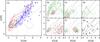 |
Fig. 2 Distributions of the known members (identified in the SIMBAD database) shown in contours on the [J] − [K] versus [K] − [9] color–color diagram: a) C-rich AGBs (red; group E), AGBs (black) and OH/IR stars (blue) (O-rich AGBs; group F); b) T Tauri (brown) and YSOs (green) (group A); c) Be stars (including Wolf-Rayet stars; brown) and emission-line stars (green) (group B); d) normal stars including O–M giants and dwarfs (green; group C); e) S-stars (green; group D), and post-AGBs and planetary nebulae (brown; group G); and f) normal and starburst galaxies (green) and Seyferts (brown) (group H). The occupation zones for the groups A–H are summarized in g). The contours show 20%, 50%, and 80% of the peak value. The SIMBAD definitions of the members of the groups A–H are summarized in Table 1. |
Classification of the AKARI/MIR catalogue sources.
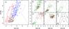 |
Fig. 3 Same as Fig. 2, but the data are instead presented on the [K] − [9] vs. [9] − [18] color–color diagram. The occupation zone for emission-line stars (B) is not defined on this diagram because they cannot be clearly separated from the other objects (panel c)). |
All the cross-identified sources are plotted on color–color diagrams. Figures 1a–c show the color–color diagrams of [J] − [K] versus (vs.) [K] − [9] , [K] − [9] vs. [9] − [18] , and [J] − [K] vs. [9] − [18] , respectively. Here, [J] , [K] , [9] , and [18] represent Vega magnitudes in the 2MASS J, 2MASS Ks, AKARI 9 μm, and AKARI 18 μm bands, respectively. The zero point magnitudes for the 9 μm and 18 μm bands are 56.3 and 12.0 Jy, respectively (Onaka et al. 2007).
We then define eight groups (A–H) and assign already known objects to the groups following the identification of the SIMBAD database as summarized in Table 1. Figures 2–4 show the distributions of the known objects on the same color–color diagrams as Figs. 1a–c, respectively. In all three diagrams, a large fraction of objects are concentrated near the origin, which represents the colors of the photospheres of normal stars. The object distribution extends to the upper-right direction for stars with warm circumstellar dust. In the diagrams including the [J] − [K] axis (i.e. Figs. 1a and c), [K] -excess objects are mixed with objects reddened by interstellar extinction. In the diagrams including the [K] − [9] axis (i.e. Figs. 1a and 1b), very red ( [K] − [9] > 5) objects, presumably dominated by hot dust emission or the emission of polycyclic aromatic hydrocarbons (PAHs), can be clearly distinguished from the majority of the objects, although they are relatively small in number.
We define the occupation zone of each class exclusively on these color–color diagrams based on the locations of the known members. The defined zones are overlaid in Figs. 2–4. Table 1 summarizes the numbers of known members used in the definition of the occupation zones, and the total number of the sources in the corresponding zones. The occupation zones defined in this work are consistent with the criteria used in the source selections in the related works using AKARI/MIR survey data (Ita et al. 2010; Takita et al. 2010).
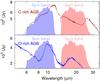 |
Fig. 5 Relative response curves of the AKARI 9 μm band and 18 μm band. The ISO/SWS spectra of typical Galactic C-rich and O-rich stars are overlaid as references (Sloan et al. 2003). An example of the C-rich star, IRC +40540, displays carbonaceous features around 11 and 30 μm, that are not covered by the AKARI bands. A typical O-rich star, oCet, shows silicate features around 10 and 18 μm, which are efficiently covered by the AKARI bands. |
The C-rich and O-rich AGB stars can be clearly distinguished in all the three color–color diagrams (Figs. 2a, 3a, and 4a). This is because the silicate features of O-rich AGB stars around 10 and 20 μm are well-covered by the AKARI 9 μm and 18 μm bands, while the carbonaceous (e.g. SiC) features of C-rich AGB stars do not contribute to these AKARI bands (Fig. 5). These characteristics are effective in helping us to differentiate C-rich from O-rich AGB stars, and their availability is one of the unique advantages of the AKARI/MIR survey data compared with the other infrared surveys of IRAS (Neugebauer et al. 1984), MSX (Price et al. 2001), and WISE (Wright et al. 2010). The distinction of C-rich from O-rich objects is clearest in the [J] − [K] vs. [9] − [18] color–color diagram (Fig. 4a). Thus, we first use the classification in the [J] − [K] vs. [9] − [18] color–color diagram (hereafter called candidate samples), and then treat the sources residing in the occupation zones in all the three color–color diagrams as more purified sub-samples (hereafter called purified samples). As a result, the candidate samples contain 18 596 C-rich and 83 012 O-rich AGB stars, while the purified samples contain 5537 C-rich and 11 416 O-rich AGB stars (Table 2).
As described above, contamination is inevitable for this type of method. We investigate the reliability and the completeness of the classified samples as follows and summarize them in Table 2. The samples located in each occupation zone are composed of four types of objects: (a) correctly classified known objects; (b) known objects that are classified as other categories, but can be regarded as the same group; (c) unknown objects; and (d) known objects that should belong to another group. The objects labeled as variable stars and infrared objects are included in (b) for C-rich and O-rich stars. Mira-type stars are also included in (b) for O-rich stars. For each occupation zone, we define (na + nb)/(na + nb + nc + nd) as a lower limit, and (na + nb + nc)/(na + nb + nc + nd) as an upper limit to the reliability of the classified samples, where na, nb, nc, and nd are the numbers of objects in (a), (b), (c), and (d), respectively. For each object class, the completeness is estimated as the ratio of the number of correctly classified known objects to the total number of known objects of the same class in the AKARI MIR PSC. The number of known objects for each class depends on the previous incomplete surveys. However, that is only the method to assess our samples, that is useful to judge the validity of the statistical results based on our samples. For the candidate samples, the reliability is 44–95% for C-rich AGB stars, and 53–95% for O-rich AGB stars. The completeness is 82% for C-rich AGB stars and 80% for O-rich AGB stars. For the purified samples, the reliability is 68–96% for C-rich AGB stars, and 71–96% for O-rich AGB stars. The completeness is 64% for C-rich AGB stars and 29% for O-rich AGB stars. The completeness for O-rich AGB stars is lower than for C-rich AGB stars. As shown in Figs. 2–4, since the O-rich and C-rich samples are bluer, they are more intermixed, whereas the redder ones in the same samples can be clearly separated. Therefore, with the present classification, it is inevitable that the completeness for the redder members is higher than that for the bluer members. Thus, the completeness of the C-rich samples is higher than that of the O-rich samples, which contain a larger numbers of lower-mass non-dusty stars.
Reliability and completeness of the newly classified C-rich and O-rich samples.
3. Results
3.1. Galactic distributions
Figure 6 shows the spatial distributions of the objects selected in the [9] − [18] vs. [J] − [K] color–color diagrams in density maps in the Galactic coordinates. The surface densities in the maps in Fig. 6 are calculated for the area of 1 × 1 deg2, and given in units of deg-2. The spatial distributions of S-stars, C-rich AGB stars, and O-rich AGB stars trace the Galactic disk. The bulge, the LMC, and the Small Magellanic Cloud (SMC) are also recognized in these maps. Dwarfs and giants (group C in Fig. 6) show relatively uniform distributions in contrast to the other populations except for two dim concentrations around l = −90° and + 90°. Since normal stars are faint in the MIR bands, their detection volume is limited to the local space (<1 kpc) around Sun. The distributions are similar to that of the Hipparcos stars (Perryman et al. 1997), corresponding to the structure of the local arm. In the panel for YSOs (group A in Fig. 6), nearby star-forming regions such as Orion, Taurus, and ρOph are recognized. These maps demonstrate the plausibility of the classification by reproducing well-known major characteristics of the spatial distribution of each Galactic object.
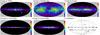 |
Fig. 6 Spatial distributions of the AKARI/MIR sources in density maps in the Galactic coordinates of the Aitoff projection. These sources are classified on the basis of the [9] − [18] vs. [J] − [K] color–color diagram alone (candidate samples). We show groups A, C, D, E, and F because they have a sufficiently large number of members. The color scales are linear from 0% to 50% of the peak value and given in units of deg-2. The coordinate grids and the locations of the Galactic bulge, the LMC, the SMC, and the nearby star-forming regions are shown in the lower right panel. |
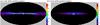 |
Fig. 7 Spatial distributions of the purified samples of a) C-rich AGB stars and b) O-rich AGB stars in density maps in the Galactic coordinates. The purified sample corresponds to those belonging to all the occupation zones of the [J] − [K] vs. [K] − [9] (Fig. 2a), [K] − [9] vs. [9] − [18] (Fig. 3a), and [J] − [K] vs. [9] − [18] diagrams (Fig. 4a). The color scales are linear from 0% to 100% of the peak value and given in units of deg-2. |
3.2. Distributions of C-rich and O-rich AGB stars
Figures 7a and b show the celestial distributions of the purified C-rich and O-rich AGB samples, respectively, as density maps in Galactic coordinates. By assuming that the star counts can be described using Poisson statistics, the 2-σ significance levels of the surface densities of the C-rich and O-rich AGB samples are 0.3 and 1.5 deg-2, respectively. The O-rich stars show a concentration toward the G.C. (the areal density varies from 3 deg-2 in the G.C. to < 0.5 deg-2 in the outer Galaxy (|l| > 90°)), whereas C-rich stars show a uniform distribution along the Galactic plane (the areal density is kept to within 0.2–0.4 deg-2 across the Galactic plane). Thus, the decrease in density along the Galactic plane seen in Fig. 7b is significant, while the small-scale structures in Fig. 7a are not. These results can be accounted for either by an intrinsic difference in the distribution on a Galactic scale, or by a situation where O-rich stars are distributed on a Galactic scale in the thin disk with interstellar extinction and C-rich stars are located in relatively nearby regions. To investigate any difference in greated detail, three-dimensional information would be indispensable.
We plot C-rich and O-rich AGB stars in the projection onto the Galactic plane of both disk stars (|b| < 10°; Figs. 8a and c) and stars at high Galactic latitudes (|b| > 10°; Figs. 8b and d). The distances of the individual samples were estimated from their AKARI 9 μm fluxes (F9 μm) and [K] − [9] colors. A formula to estimate the distances was empirically derived using the sub-samples for which the distance and the mass-loss rates were known. These parameters were estimated based on MIR observations independently by Zhang et al. (2010) and Le Bertre et al. (2003). We derived the relation among the distance, the mass-loss rates, and F9 μm for the sub-samples. We also derived the relation between the mass-loss rates and [K] − [9] colors (see Appendix for details of the derivation). By combining both relations, we obtained a formula to derive the distance from F9 μm and [K] − [9] . The maximum distance that we can probe in our sample is limited by the detection limit for the AKARI 18 μm flux. The maximum distance to the faintest members in our sample is estimated to be 8 ± 2 kpc, based on the above flux-distance relation with typical [9] − [18] colors (also see Appendix).
The edge of the outer part of our Galaxy (the left side of Fig. 8) indicates the end of the corresponding stellar populations, whereas the edge toward the direction of the opposite side over the G.C. (the right side of Fig. 8) corresponds to the detection limit of this survey for the corresponding objects. The elliptical concentration is seen around the G.C. in the panels for the disk component (|b| < 10°; Figs. 8a and c). The inclination of about five degrees to the Sun–G.C. axis may indicate the central bar (Genhard 2002; Cole & Weinberg 2002). However, we note that the elongated distribution is also caused by the uncertainties in the derived distances to the individual stars. The concentrations of sources around l ~ 280–300° in the panels for high latitude objects (|b| > 10°; Figs. 8b and d) indicate the LMC and the SMC. They are clearly separated from our Galaxy, though there remains an elongated distribution towards the LMC presumably caused by the errors in the distance estimates.
The most remarkable finding is that O-rich AGB stars are concentrated toward the G.C. while C-rich AGB stars have a relatively uniform distribution across the Galactic disk.
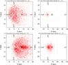 |
Fig. 8 Spatial distributions of the C-rich and O-rich AGB stars projected onto the Galactic plane viewed from the north pole: a) C-rich AGBs at |b| ≤ 10°, b) C-rich AGBs at |b| > 10°, c) O-rich AGBs at |b| ≤ 10°, and d) O-rich AGBs at |b| > 10°. The red dots indicate the purified samples. The contours in panels a) and c) show the areal densities for the purified samples (i.e. densities of red points). The levels of the contours are 10, 20, and 30 kpc-2 for panel a), and 10, 50, and 100 kpc-2 for panel c). The distance scale for each object is estimated from the AKARI 9 μm fluxes and [K] − [9] colors (see Sect. 3). The Sun is located at the origin. The G.C. is to the right of the Sun and shown by the cross at (X,Y) = (8.5,0). The dotted squares in b) and d) indicate the size of a) and c). Note that the scale of the distance used in panels b) and d) is a factor of two larger than that in panels a) and c). |
4. Discussion
To have more quantitative discussion about the difference in the spatial distributions of C-rich and O-rich AGB stars, we plot the areal number density of our samples as a function of Galactocentric distance (Rg) in Fig. 9. At various galactocentric distances, we count the numbers of disk AGB stars included in the annular regions of width 0.3 kpc within 8 kpc of the Sun considering the survey depth. The smaller errors indicated by darkly colored stripes in Fig. 9 are estimated by the Poisson statistics in the star counts, while the larger ones indicated by more lightly colored stripes include an uncertainty of ± 2 kpc in estimating the distance. We also investigate the completeness of both samples as a function of Rg in the lower panel of Fig. 9. The completeness of the C-rich sample increases with Rg, while that of the O-rich sample is lower in the outer galaxy (Rg > 9 kpc). For O-rich AGB stars, the completeness is higher for the redder members (see Sect. 2). The lower completeness in outer Galaxy means that the fraction of dusty members (i.e. massive O-rich AGB stars) becomes smaller in the outer Galaxy. In contrast, the completeness of the C-rich AGB stars shows little depends on their color. The number and variety of the catalogued C-rich AGB stars are relatively small in the outer Galaxy. Thus, the completeness of C-rich AGB stars increases toward the outer Galaxy. The ratio of the completeness of the C-rich sample to that of the O-rich sample is found to be almost constant at Rg < 9 kpc. Hence, our result is not affected much by the variations in the completeness.
Table 3 summarizes the related investigations with the numbers and the penetrating depths of the samples. Previous studies have consistently reported relatively flat distributions of C-rich AGB samples compared with O-rich AGB samples, which are instead concentrated toward the G.C. Our result in Fig. 9 quantitatively confirms the trends reported in the previous works, which improves the spatial completeness by extending the survey volume to 8 kpc from the Sun and avoiding source confusions toward the G.C.
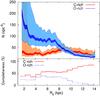 |
Fig. 9 Upper panel: areal densities of the number of the purified C-rich (red) and the O-rich (blue) AGB samples in the Galactic plane (|b| < 10°) as a function of Galactocentric distance (Rg), not corrected for the completeness (see below). For each Rg, we count the numbers of the disk AGB stars included in the annular regions of width 0.3 kpc within 8 kpc of Sun (the penetrating depth of our sample) and divide the star counts by the corresponding areas. The narrower stripes indicate the errors estimated from the Poisson statistics for the star counts, while the wider stripes indicate the ones derived by assuming uncertainties of ± 2 kpc in estimating the distance. Lower panel: completeness of both samples as a function of the Galactocentric distance (Rg). |
Related investigations of the spatial distribution of C-rich AGBs.
Why do the distributions of C-rich and O-rich AGB stars differ? One possible reason is that the metallicity of the ISM at their birth place affects the stellar chemical composition of the photospheres (e.g. Noguchi et al. 2004). The metallicity gradient along Rg was reported by many authors (e.g. by using Cepheids and open clusters). The reported gradient of d [Fe/H] /dRg at Rg = 5–15 kpc varies from −0.04 to −0.13 dex kpc-1 (Pedicelli et al. 2009), and is higher toward the inner Galaxy. The [O/H] gradients are also reported by several authors (e.g. Smartt & Rolleston 1997; Shaver et al. 1983; Rudolph et al. 2006), to be between about −0.04 and −0.07 dex kpc-1 at radii 6–18 kpc. The log(C/M) value at radii Rg = 2 to 14 kpc in our result has the gradient of ~0.1 dex kpc-1, which has an inverse gradient of slope similar in absolute value to that of the metallicity.
The anti-correlation between the metallicity and the C/M ratio is also reported for nearby galaxies. Brewer et al. (1995) reported on M 31, a spiral galaxy similar to our Galaxy, observing five regions located at 4–32 kpc from the G.C. The metallicity decreases along the Rg, whereas the C/M ratio increases. Pritchet et al. (1987) confirmed that the number of C-rich AGB stars per unit luminosity shows a correlation with the average [Fe/H] among the galaxies, IC 1613, SMC, NGC 6822, NGC55, M 33, LMC, NGC 300, M 31, and our Galaxy, thus the lower metallicity results in the higher C/M ratio. The relation is approximated by d( [Fe/H] )/d(log (C/M)) ~ −0.5 (e.g. Battinelli & Demers 2005; Cioni 2009). Our result in Fig. 9 shows that the slope is d( [Fe/H] )/d(log (C/M)) = −0.4 ~ −1.3 at R = 2–14 kpc, which connects smoothly with the value for nearby galaxies. Thus, the trend reported in nearby galaxies is applicable to our Galaxy, while the ranges of metallicity are different: −1.3 < [Fe/H] < 0 for nearby galaxies, and −0.5 < [Fe/H] < 1 for our Galaxy. We note that the metallicity dependence of the C/M ratio in nearby galaxies is based on optical (Battinelli & Demers 2005) or near-infrared (NIR; Cioni 2009) observations, whereas our result is based on MIR observations. Figure 9 also suggests that C/M ~ 1 at [Fe/H] = 0 (i.e. the solar abundance), although our O-rich samples are biased toward dusty members.
How does the difference in spatial distributions between C-rich and O-rich AGB stars affect the ISM in our Galaxy? Our result indicates that as dust suppliers the population of C-rich stars are minor contributers in the inner Galaxy but major contributors around the Sun and in the outer Galaxy. It is reasonable to assume that the mass loss from AGB stars has a direct effect on the chemical composition of their local ISM. The spatial constraint on the dominant replenishment of carbonaceous grains to the ISM may have implications for habitable zones in our Galaxy (Guillermo et al. 2001), though a significant theoretical gap remains between the supply of carbonaceous grains to the interstellar space and the origin of organic material. The spatial variation in the amount of interstellar carbonaceous grains relative to that of silicate grains has not been reported on the Galactic scale. Furthermore, it is well-known that the PAH (as a representative of carbonaceous grain) emission displays a good spatial correlation with the cold dust emission (e.g. Onaka et al. 1996; Draine et al. 2007; Bendo et al. 2008); the latter is mostly emitted by silicate grains. We plan to perform detailed and quantitative comparisons of the spatial distributions of carbonaceous and silicate grains with those of C-rich and O-rich AGB stars in our Galaxy in future work.
5. Summary
On the bassis of AKARI observations, we have investigated the spatial distributions of C-rich and O-rich AGB stars in our Galaxy. The C-rich and O-rich AGB stars in the AKARI 9 μm and 18 μm All-Sky Survey catalogue are well-distinguished by the empirical approach using color–color diagrams. The reliability and the completeness of the sample selection are discussed. The C-rich AGB stars are uniformly distributed within 8 kpc from Sun, while O-rich AGB stars are concentrated toward the G.C. Our result confirms those of previous investigations, extends the survey volume to the Galactic scale (~8 kpc), and enhances the completeness toward the inner Galaxy by spatially resolving individual sources. We also propose that the metallicity gradient with galactocentric distance can be one of the possible origins of the difference in the spatial distributions of C-rich and O-rich AGB stars.
Acknowledgments
This work was supported by the the Nagoya University Global COE Program, “Quest for Fundamental Principles in the Universe (QFPU)” from JSPS and MEXT of Japan. This research is based on observations with AKARI, a JAXA project with the participation of ESA. We thank all the members of the AKARI project. This research has made use of the SIMBAD database, operated at CDS, Strasbourg, France. This publication makes use of data products from the Two Micron All Sky Survey, which is a joint project of the University of Massachusetts and the Infrared Processing and Analysis Center/California Institute of Technology, funded by the National Aeronautics and Space Administration and the National Science Foundation. This research has made use of the NASA/IPAC Infrared Science Archive, which is operated by the Jet Propulsion Laboratory, California Institute of Technology, under contract with the National Aeronautics and Space Administration. We also thank an anonymous referee for careful reading and constructive comments.
References
- Battinelli, P., & Demers, S. 2005, A&A, 434, 657 [NASA ADS] [CrossRef] [EDP Sciences] [Google Scholar]
- Bendo, G. J., Draine, B. T., Engelbracht, C. W., et al. 2008, MNRAS, 389, 629 [NASA ADS] [CrossRef] [Google Scholar]
- Bertoldi, F., Carilli, C. L., Cox, P., et al. 2003, A&A, 406, L55 [NASA ADS] [CrossRef] [EDP Sciences] [Google Scholar]
- Blanco, V. M. 1965, in Stars and Stellar Systems, ed. A. Blaauw, & M. Schmidt (Chicago: University of Chicago Press), Vol. V, 241 [Google Scholar]
- Brewer, J. P., Richer, H. B., & Crabtree, D. R. 1995, AJ, 109, 2480 [NASA ADS] [CrossRef] [Google Scholar]
- Buchanan, C. L., Kastner, J. H., Hrivnak, B. J., & Sahai, R. 2009, AJ, 138, 1597 [NASA ADS] [CrossRef] [Google Scholar]
- Chen, P. S., Szczerba, R., Kwok, S., & Volk, K. 2001, A&A, 368, 1006 [NASA ADS] [CrossRef] [EDP Sciences] [Google Scholar]
- Cioni, M.-R. L. 2009, A&A, 506, 1137 [NASA ADS] [CrossRef] [EDP Sciences] [Google Scholar]
- Claussen, M. J., Kleinmann, S. G., Joyce, R. R., & Jura, M. 1987, ApJS, 65, 385 [NASA ADS] [CrossRef] [Google Scholar]
- Cole, A. A., & Weinberg, M. D. 2002, ApJ, 574, 43 [Google Scholar]
- Draine, B. T., Dale, D. A., Bendo, G., et al. 2007, ApJ, 663, 866 [NASA ADS] [CrossRef] [Google Scholar]
- Egan, M. P., Van Dyk, S. D., & Price, S. D. 2001, AJ, 122, 1844 [NASA ADS] [CrossRef] [Google Scholar]
- Gerhard, O. 2002, The Dynamics, Structure & History of Galaxies, ed. G. S. Da Costa, & H. Jerjen (San Francisco, CA: ASP), ASP Conf. Ser., 273, 73 [Google Scholar]
- Guillermo, G., Donald, B., & Peter, W. 2001, Icarus, 152, 185 [NASA ADS] [CrossRef] [Google Scholar]
- Habing, H. J., Olnon, F. M., Chester, T., Gillett, F., & Rowan-Robinson, M. 1985, A&A, 152, 1 [Google Scholar]
- Ishihara, D., Wada, T., Onaka, T., et al. 2006, PASP, 118, 324 [NASA ADS] [CrossRef] [Google Scholar]
- Ishihara, D., Onaka, T., Kataza, H., et al. 2010a, A&A, 514, A1 [NASA ADS] [CrossRef] [EDP Sciences] [Google Scholar]
- Ishihara, D., Kaneda, H., Furuzawa, A., et al. 2010b, A&A, 521, L61 [NASA ADS] [CrossRef] [EDP Sciences] [Google Scholar]
- Ita, Y., Matsuura, M., Ishihara, D., et al. 2010, A&A, 514, A2 [NASA ADS] [CrossRef] [EDP Sciences] [Google Scholar]
- Jura, M., & Kleinmann, S. G. 1990, ApJ, 364, 663 [NASA ADS] [CrossRef] [Google Scholar]
- Le Bertre, T., Tanaka, M., Yamamura, I., & Murakami, H. 2003, A&A, 403, 943 [NASA ADS] [CrossRef] [EDP Sciences] [Google Scholar]
- Lee, H. G., Koo, B. C., Moon, D. S., et al. 2009, ApJ, 706, 441 [NASA ADS] [CrossRef] [Google Scholar]
- Lumsden, S. L., Hoare, M. G., Oudmaijer, R. D., & Richards, D. 2002, MNRAS, 336, 621 [NASA ADS] [CrossRef] [Google Scholar]
- Matsuura, M., Barlow, M. J., Zijlstra, A. A., et al. 2009, MNRAS, 396, 918 [NASA ADS] [CrossRef] [Google Scholar]
- Murakami, H., Freund, M. M., Ganga, K., et al. 1996, PASJ, 48, L41 [NASA ADS] [CrossRef] [Google Scholar]
- Murakami, H., Baba, H., Barthel, P., et al. 2007, PASJ, 59, 369 [Google Scholar]
- Neugebauer, G., & Leighton, R. B. 1969, Two Micron Sky Survey, NASA SP-2047, TMSS [Google Scholar]
- Neugebauer, G., Habing, H. J., van Duinen, R., et al. 1984, ApJ, 278, 1 [NASA ADS] [CrossRef] [Google Scholar]
- Noda, M., Matsumoto, T., Murakami, H., et al. 1996, Proc. SPIE, 2817, 248 [NASA ADS] [CrossRef] [Google Scholar]
- Noguchi, K., Aoki, W., & Kawanomoto, S. 2004, A&A, 418, 67 [NASA ADS] [CrossRef] [EDP Sciences] [Google Scholar]
- Onaka, T., Yamamura, I., Tanabe, T., Roellig, T. L., & Yuen, L. 1996, PASJ, 48, 59 [Google Scholar]
- Onaka, T., Matsuhara, H., Wada, T., et al. 2007, PASJ, 59, S401 [Google Scholar]
- Pedicelli, S., Bono, G., Lemasle, B., et al. 2009, A&A, 504, 81 [NASA ADS] [CrossRef] [EDP Sciences] [Google Scholar]
- Pritchet, C. J., Schade, D., Richer, H. B., Crabtree, D., & Yee, H. K. C. 1987, ApJ, 323 79 [Google Scholar]
- Perryman, M. A. C., Lindegren, L., Kovalevsky, J., et al. 1997, A&A, 323, 49 [Google Scholar]
- Price, S. D., Egan, M. P., Carey, S. J., et al. 2001, AJ, 121, 2819 [NASA ADS] [CrossRef] [Google Scholar]
- Rho, J., Kozasa, T., Reach, W. R., et al. 2008, ApJ, 673, 271 [NASA ADS] [CrossRef] [Google Scholar]
- Rudolph, A. L., Fich, M. B., Gwendolyn, R., et al. 2006, ApJS, 162, 346 [NASA ADS] [CrossRef] [Google Scholar]
- Shaver, P. A., McGee, R. X., Newton, L. M., Danks, A. C., & Pottasch, S. R. 1983, MNRAS, 204, 53 [NASA ADS] [CrossRef] [Google Scholar]
- Skrutskie, M. F., Cutri, R. M., Stiening, R., et al. 2006, AJ, 131, 1163 [NASA ADS] [CrossRef] [Google Scholar]
- Sloan, G. C., Kraemer, K. E., Price, S. D., & Shipman, R. F. 2003, ApJS, 147, 379 [NASA ADS] [CrossRef] [Google Scholar]
- Smartt, S. J., & Rolleston, W. R. J. 1997, ApJ, 481, 47 [Google Scholar]
- Takita, S., Kataza, H., Kitamura, Y., et al. 2010, A&A, 519, A83 [NASA ADS] [CrossRef] [EDP Sciences] [Google Scholar]
- Taylor, J. H., & Cordes, J. M. 1993, ApJ, 411, 674 [NASA ADS] [CrossRef] [Google Scholar]
- Thronson, H. A., Jr., Latter, W. B., Black, J. H., Bally, J., & Hacking, P. 1987, ApJ, 322, 770 [NASA ADS] [CrossRef] [Google Scholar]
- van der Veen, W. E. C. J., & Habing, H. J. 1988, A&A, 194, 125 [NASA ADS] [Google Scholar]
- Walker, H. J., & Cohen, M. 1988, AJ, 95, 1801 [NASA ADS] [CrossRef] [Google Scholar]
- Walker, H. J., Volk, K., Wainscoat, R. J., et al. 1989, AJ, 98, 2163 [NASA ADS] [CrossRef] [Google Scholar]
- Weingartner, J. C., & Draine, B. T. 2001, ApJ, 548, 296 [NASA ADS] [CrossRef] [Google Scholar]
- Westerlund, B. E. 1965, MNRAS, 130, 45 [NASA ADS] [Google Scholar]
- Wright, E. L., Eisenhardt, P. R. M., Mainzer, A. K., et al. 2010, AJ, 140, 1868 [NASA ADS] [CrossRef] [Google Scholar]
- Zhang, H., Zhou, J., Dong, G., Esimbek, J., & Mu, J. 2010, Ap&SS, 330, 23 [NASA ADS] [CrossRef] [Google Scholar]
Appendix A: Distance estimate
We first derive an empirical relation between the distance (D; kpc), the observed 9 μm flux (F9 μm; Jy), and the [K] − [9] color for well-studied AGB samples (Le Bertre et al. 2003; Zhang et al. 2010). We then apply this relation to our samples and estimate D from the observed values of F9 μm and [K] − [9] . We use AKARI 9 μm fluxes because they are more acurate than the 18 μm fluxes.
The Le Bertre et al. (2003) sample contains 126 C-rich stars and 563 O-rich stars observed by the IRTS/NIRS. The Zhang et al. (2010) sample contains 184 C-rich stars and 110 O-rich stars selected from the literature. Most members of both samples have AKARI 9 μm fluxes. The mass-loss rates for both samples are estimated observationally by using methods independent of MIR observations, while the distances are estimated based on NIR and MIR fluxes. The mixture of these samples (hereafter BZ sample) comprehensively covers both dust-poor members (10-7.5 − 10-5.5 M⊙ yr-1) and dust-rich members (10-5.5 − 10-4 M⊙ yr-1).
Figure A.1 shows the distances vs. the AKARI 9 μm fluxes for the BZ sample. The observed flux is inversely proportional to the square of the distance,  (A.1)where L9 μm is the intrinsic luminosity of a star at 9 μm. We assume that L9 μm is a function of the amount of circumstellar dust, thus a function of the mass-loss rate (dM/dt; M⊙ yr-1) as
  (A.2)where γ is a free parameter.
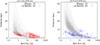 |
Fig. A.1 a) Heliocentric distance of C-rich AGB stars as a function of the AKARI 9 μm flux. The open squares and the open circles show previously measured distances for well-studied samples from Zhang et al. (2010, squares) and Le Bertre et al. (2003, circles), respectively. The black dots show distances estimated for our purified samples. The dashed curves indicate the luminosity distance for the objects of [K] − [9] = 14 mag and [K] − [9] = 1 mag, which correspond to the dust-rich case (dM/dt ~ 10-4 M⊙ yr-1) and the dust-poor case (dM/dt ~ 10-8 M⊙ yr-1), respectively (see Fig. A.2). The vertical lines indicate the faint flux end of our sample (270 |

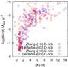 |
Fig. A.2 Mass-loss rate of AGB stars as a function of the [K] − [9] color, measured by Zhang et al. (2010) and Le Bertre et al. (2003). The symbols are the same as in Fig. A.1. |
By combining Eqs. (A.1) and (A.2), the distance is described as a function of F9 μm and dM/dt as  (A.3)where C1 and C2 are obtained as 6.1 ± 0.06, and 0.35 ± 0.01, respectively, by fitting the linear relation among log (D), log (dM/dt), and log (F9 μm) for the BZ sample.
To obtain dM/dt from our observations, we assume that it is a function of excess emission indicated by the [K] − [9] color. Figure A.2 shows the mass-loss rate plotted against [K] − [9] color for the BZ sample. We assume that the dotted curve in Fig. A.2, is an empirical relation between the mass loss rate and the color expressed as ![Mathematical equation: \appendix \setcounter{section}{1} \begin{equation} \log({\rm d}M/{\rm d}t) = \log(3.8\times(([K]-[9])-0.4))-8.0 . \end{equation}](/articles/aa/full_html/2011/10/aa17626-11/aa17626-11-eq99.png) (A.4)From Eqs. (A.3) and (A.4) with observed F9 μm and [K] − [9] , we estimate the distances of our sample. The results are overlaid with dots in Fig. A.1. The faintest F9 μm of our sample is limited by the detection limit of the AKARI 18 μm band. Typical [9] − [18] colors for dust-poor AGBs are 0.5 ± 0.5 mag from Fig. 3a. By applying them to the flux detection limit at 18 μm (90 mJy; Ishihara et al. 2010a), the minimum F9μm for our sample is 270
(A.4)From Eqs. (A.3) and (A.4) with observed F9 μm and [K] − [9] , we estimate the distances of our sample. The results are overlaid with dots in Fig. A.1. The faintest F9 μm of our sample is limited by the detection limit of the AKARI 18 μm band. Typical [9] − [18] colors for dust-poor AGBs are 0.5 ± 0.5 mag from Fig. 3a. By applying them to the flux detection limit at 18 μm (90 mJy; Ishihara et al. 2010a), the minimum F9μm for our sample is 270 mJy, which corresponds to the distance of 8 ± 2 kpc from Fig. A.1. Figure A.1 also indicates that the AKARI/MIR survey can probe dust-rich AGB stars beyond 40 kpc, covering the objects in the LMC and the SMC.
All Tables
All Figures
|
Fig. 1 Color–color diagrams in density maps for the AKARI/MIR sources that have 2MASS measurements: a) [J] − [K] versus [K] − [9] , b) [K] − [9] versus [9] − [18] , and c) [J] − [K] versus [9] − [18] color–color diagrams. The arrow on each panel shows the interstellar extinction vector for AV = 20 mag, by using the Weingartner & Draine (2001) Milky Way model of RV = 3.1. The color scales of the maps are logarithmic in number per unit color space. (The color versions of this and subsequent figures are available in the online journal.) |
| In the text | |
|
Fig. 2 Distributions of the known members (identified in the SIMBAD database) shown in contours on the [J] − [K] versus [K] − [9] color–color diagram: a) C-rich AGBs (red; group E), AGBs (black) and OH/IR stars (blue) (O-rich AGBs; group F); b) T Tauri (brown) and YSOs (green) (group A); c) Be stars (including Wolf-Rayet stars; brown) and emission-line stars (green) (group B); d) normal stars including O–M giants and dwarfs (green; group C); e) S-stars (green; group D), and post-AGBs and planetary nebulae (brown; group G); and f) normal and starburst galaxies (green) and Seyferts (brown) (group H). The occupation zones for the groups A–H are summarized in g). The contours show 20%, 50%, and 80% of the peak value. The SIMBAD definitions of the members of the groups A–H are summarized in Table 1. |
| In the text | |
|
Fig. 3 Same as Fig. 2, but the data are instead presented on the [K] − [9] vs. [9] − [18] color–color diagram. The occupation zone for emission-line stars (B) is not defined on this diagram because they cannot be clearly separated from the other objects (panel c)). |
| In the text | |
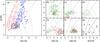 |
Fig. 4 Same as Fig. 2, but shown on the [J] − [K] vs. [9] − [18] color–color diagram. |
| In the text | |
|
Fig. 5 Relative response curves of the AKARI 9 μm band and 18 μm band. The ISO/SWS spectra of typical Galactic C-rich and O-rich stars are overlaid as references (Sloan et al. 2003). An example of the C-rich star, IRC +40540, displays carbonaceous features around 11 and 30 μm, that are not covered by the AKARI bands. A typical O-rich star, oCet, shows silicate features around 10 and 18 μm, which are efficiently covered by the AKARI bands. |
| In the text | |
|
Fig. 6 Spatial distributions of the AKARI/MIR sources in density maps in the Galactic coordinates of the Aitoff projection. These sources are classified on the basis of the [9] − [18] vs. [J] − [K] color–color diagram alone (candidate samples). We show groups A, C, D, E, and F because they have a sufficiently large number of members. The color scales are linear from 0% to 50% of the peak value and given in units of deg-2. The coordinate grids and the locations of the Galactic bulge, the LMC, the SMC, and the nearby star-forming regions are shown in the lower right panel. |
| In the text | |
|
Fig. 7 Spatial distributions of the purified samples of a) C-rich AGB stars and b) O-rich AGB stars in density maps in the Galactic coordinates. The purified sample corresponds to those belonging to all the occupation zones of the [J] − [K] vs. [K] − [9] (Fig. 2a), [K] − [9] vs. [9] − [18] (Fig. 3a), and [J] − [K] vs. [9] − [18] diagrams (Fig. 4a). The color scales are linear from 0% to 100% of the peak value and given in units of deg-2. |
| In the text | |
|
Fig. 8 Spatial distributions of the C-rich and O-rich AGB stars projected onto the Galactic plane viewed from the north pole: a) C-rich AGBs at |b| ≤ 10°, b) C-rich AGBs at |b| > 10°, c) O-rich AGBs at |b| ≤ 10°, and d) O-rich AGBs at |b| > 10°. The red dots indicate the purified samples. The contours in panels a) and c) show the areal densities for the purified samples (i.e. densities of red points). The levels of the contours are 10, 20, and 30 kpc-2 for panel a), and 10, 50, and 100 kpc-2 for panel c). The distance scale for each object is estimated from the AKARI 9 μm fluxes and [K] − [9] colors (see Sect. 3). The Sun is located at the origin. The G.C. is to the right of the Sun and shown by the cross at (X,Y) = (8.5,0). The dotted squares in b) and d) indicate the size of a) and c). Note that the scale of the distance used in panels b) and d) is a factor of two larger than that in panels a) and c). |
| In the text | |
|
Fig. 9 Upper panel: areal densities of the number of the purified C-rich (red) and the O-rich (blue) AGB samples in the Galactic plane (|b| < 10°) as a function of Galactocentric distance (Rg), not corrected for the completeness (see below). For each Rg, we count the numbers of the disk AGB stars included in the annular regions of width 0.3 kpc within 8 kpc of Sun (the penetrating depth of our sample) and divide the star counts by the corresponding areas. The narrower stripes indicate the errors estimated from the Poisson statistics for the star counts, while the wider stripes indicate the ones derived by assuming uncertainties of ± 2 kpc in estimating the distance. Lower panel: completeness of both samples as a function of the Galactocentric distance (Rg). |
| In the text | |
|
Fig. A.1 a) Heliocentric distance of C-rich AGB stars as a function of the AKARI 9 μm flux. The open squares and the open circles show previously measured distances for well-studied samples from Zhang et al. (2010, squares) and Le Bertre et al. (2003, circles), respectively. The black dots show distances estimated for our purified samples. The dashed curves indicate the luminosity distance for the objects of [K] − [9] = 14 mag and [K] − [9] = 1 mag, which correspond to the dust-rich case (dM/dt ~ 10-4 M⊙ yr-1) and the dust-poor case (dM/dt ~ 10-8 M⊙ yr-1), respectively (see Fig. A.2). The vertical lines indicate the faint flux end of our sample (270 |
| In the text | |
|
Fig. A.2 Mass-loss rate of AGB stars as a function of the [K] − [9] color, measured by Zhang et al. (2010) and Le Bertre et al. (2003). The symbols are the same as in Fig. A.1. |
| In the text | |
Current usage metrics show cumulative count of Article Views (full-text article views including HTML views, PDF and ePub downloads, according to the available data) and Abstracts Views on Vision4Press platform.
Data correspond to usage on the plateform after 2015. The current usage metrics is available 48-96 hours after online publication and is updated daily on week days.
Initial download of the metrics may take a while.