| Issue |
A&A
Volume 534, October 2011
|
|
|---|---|---|
| Article Number | A18 | |
| Number of page(s) | 10 | |
| Section | Stellar structure and evolution | |
| DOI | https://doi.org/10.1051/0004-6361/201116999 | |
| Published online | 22 September 2011 | |
Sirius A: turbulence or mass loss?⋆
1
LUTH, Observatoire de Paris, CNRS, Université Paris Diderot, 5 place Jules Janssen, 92190 Meudon, France
2
Département de Physique, Université de Montréal, Montréal, PQ, H3C 3J7, Canada
e-mail: michaudg@astro.umontreal.ca; jacques.richer@umontreal.ca; mathieu.vick@umontreal.ca;
Received: 31 March 2011
Accepted: 25 July 2011
Context. Abundance anomalies observed in a fraction of A and B stars of both Pop I and II are apparently related to internal particle transport.
Aims. Using available constraints from Sirius A, we wish to determine how well evolutionary models including atomic diffusion can explain observed abundance anomalies when either turbulence or mass loss is used as the main competitor to atomic diffusion.
Methods. Complete stellar evolution models, including the effects of atomic diffusion and radiative accelerations, have been computed from the zero age main-sequence of 2.1 M⊙ stars for metallicities of Z0 = 0.01 ± 0.001, and shown to closely reproduce the observed parameters of Sirius A. Surface abundances were predicted for three values of the mass loss rate and four values of the mixed surface zone.
Results. A mixed mass of ~10-6 M⊙or a mass loss rate of 10-13 M⊙/yr were determined through comparison with observations. There are 17 abundances that were determined observationally and that are included in our calculations. Up to 15 of them can be predicted to within 2σ; three of the four determined upper limits are compatible.
Conclusions. While the abundance anomalies can be reproduced slightly better using turbulence as the process competing with atomic diffusion, mass loss probably ought to be preferred since the mass loss rate required to fit abundance anomalies is compatible with the observationally determined rate. A mass loss rate within a factor of 2 of 10-13 M⊙/yr is preferred. This restricts the range of the directly observed mass loss rate.
Key words: stars: evolution / stars: abundances / stars: mass-loss / stars: chemically peculiar / diffusion
Appendices are available in electronic form at http://www.aanda.org
© ESO, 2011
1. Astrophysical context
The brightest star in the sky, Sirius A, has all its main parameters such as mass, luminosity, and age relatively well determined. Its chemical abundances have now been studied in great detail using Space Telescope data by Landstreet (2011), where more background information can be found.
In previous work (Richer et al. 2000), the then available observations of Sirius were compared with results from a grid of models calculated with atomic diffusion and turbulence as a competing process. Given the range of abundances observed for any given species, the agreement seemed satisfactory. In Vick et al. (2010), similar results were obtained through a similar approach but with mass loss as the competing process. Because the observational error bars were too large, these authors were unable to delineate which of mass loss or turbulence was responsible for its abundance anomalies.
It is currently uncertain whether turbulence or mass loss is most efficient in competing with atomic diffusion in A stars. For O and early B stars, mass loss is most likely the dominant process. It is clearly observed in those stars at a rate sufficient to obliterate the effects of atomic diffusion. However, in main-sequence A stars the expected mass loss rate produced by radiative accelerations is smaller than in O stars by several orders of magnitude. Mass loss is likely to occur only if started by another mechanism (Abbott 1982), and might involve only metals (Babel 1995). On the other hand, since surface convection zones are very thin, one expects little corona driven flux as observed on the Sun. It is then a priori quite uncertain if A stars have any mass loss. The claimed mass loss rate for Sirius is an important observation. It is thus important to verify as precisely as possible if it is compatible with current observed abundance anomalies on the surface of Sirius.
The measurement of the mass loss rate of Sirius is a difficult observation and awaited Hubble Space Telescope measurements of the Mg II resonance lines by Bertin et al. (1995). Their analysis of this spectral feature with a wind model leads to an uncertainty of 0.5 dex on the mass loss rate if Mg is all singly ionized. However there is an additional uncertainty related to the evaluation of the fraction of Mg that is singly ionized. Their more credible evaluation of Mg ionization was based on setting the ionization rate equal to the recombination rate which then led to1:  (1)On the other hand, turbulence has often been used in stellar evolution calculations to explain observed abundance anomalies. In F stars of clusters, turbulence could be responsible for the destruction of surface Li (Talon & Charbonnel 1998, 2005), thereby leading to the so-called Li gap. Turbulence could also be responsible for reducing abundance anomalies caused by atomic diffusion on Am and Fm stars (Talon et al. 2006). It can naturally explain the disappearance of abundance anomalies as rotation increases in those objects. It could also play a role in the Li abundance evolution of solar type stars (Pinsonneault et al. 1989; Proffitt & Michaud 1991). It is however always necessary to use a number of adjustable parameters in the physical models of turbulent transport and the role of turbulence remains uncertain. In this series of papers on the role of atomic diffusion in stellar evolution, turbulence was indeed only introduced when models including atomic diffusion led to anomalies larger than observed. Only one parameter was adjusted to control the influence of turbulence in limiting the size of anomalies: the surface mixed mass (Richer et al. 2000; Michaud et al. 2011).
It is possible to improve what we learn from the acccurate observations of Sirius by making more precise evolutionary calculations. Instead of the grid of solar metallicity models used in both Richer et al. (2000) in Vick et al. (2010), this paper uses two new series of models that were respectively computed with turbulence and with mass loss as the process competing with atomic diffusion. These two series are precisely converged to the known properties of Sirius, L, Teff, R, M and age. The original metallicity is determined and the predictions of models with this metallicity are then compared with observed abundances. This allows a more precise and rigorous test than the calculations using grids of models.
In this paper, stellar evolution models with atomic diffusion as described in Richer et al. (2000) and in Vick et al. (2010) are used to determine the original metallicity of Sirius A using the age, radius and mass as constraints (Sect. 2). Using this metallicity and the determined parameters, complete evolutionary models are then calculated (Sect. 3), and the surface abundances are compared with Landstreet’s observations (Sect. 4). The results are discussed in Sect. 5.
2. Original metallicity
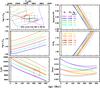 |
Fig. 1 An HR diagram and the time evolution of Teff, L, log g, R, and Zsurf are shown. Observationally determined ± 1σ intervals are shown for L, Teff, g, and R. For Teff, the spectroscopically determined error bar is in black, while that determined using luminosity and radius is in red (see the text). Each model is color coded and identified on the figure. The adopted acceptable age range is from 200 to 250 Myr (see the text). In the HR diagram, the part of the curves between 200 and 250 Myr is solid; it is dotted outside that interval. All models were calculated with turbulence. Models with mass loss could not be distinguished, in the HR diagram, from those of the same original mass and composition calculated with turbulence. A subset of the curves is shown in Fig. A.1. |
The fundamental parameters required to carry out stellar evolution calculations, excluding the original chemical composition, have been relatively well-determined for Sirius A. The Hipparcos parallax can be used to determine its distance and when coupled with interferometry (Kervella et al. 2003) to determine its radius, 1.711 ± 0.013 R⊙. Kervella et al. also use the Hipparcos parallax to determine the luminosity from the magnitude and to refine the mass determination to 2.12 ± 0.06 M⊙. From the luminosity and radius, one can infer that Teff = 9900 ± 140 K, while from spectroscopy Lemke (1989) obtained Teff = 9900 ± 200 K. The age of Sirius was discussed in Sect. 4.1 of Richer et al. (2000); using evolutionary time scales of Sirius B, they suggested that the star’s age is 250 ± 50 Myr. We adopt the slightly more restrictive range 225 ± 25 Myr suggested by Kervella et al. (2003) in their Sect. 2.2, where they argue that Sirius B would have been more massive on the main-sequence than assumed by Richer et al. (2000). Since the mass is well-determined, we use a fixed mass of 2.1 M⊙, and then evolve models with a range of metallicities, using a scaled solar mix as given in Table 1 of Turcotte et al. (1998). Helium was adjusted to the fitted solar value for model H of Turcotte et al. (1998) as starting homogeneous composition for some of the calculations. For most of the calculations, however, the He mass fraction was corrected by ΔY = −0.02 dex because of the lower final metallicity2.
In this paper, we often use a solar mass fraction, X⊙, in particular to normalize both observed and calculated mass fractions. These values are taken from Table 1 of Turcotte et al. (1998) and correspond to the solar mass fractions at the birth of the Sun, more precisely the Z0( = 0.01999) for model H in Table 6 of that paper. The surface solar abundances of metals today are some 10% smaller. Those normalizing factors differ from the solar abundances used by Landstreet for comparative purposes. Since, in this paper, the same normalizing factors are used for both observed and calculated quantities, they do not influence the comparison.
Age, luminosity, Teff, and radius are assumed to be well-determined and are used as constraints to determine the original metallicity using models with turbulence. In Fig. 1, only models with Z0 = 0.009, 0.010, and 0.011 are seen to satisfy all constraints within the predetermined error boxes. The radius is generally satisfied only for models younger than 250 Myr. Furthermore, only models with the He mass fraction reduced by 0.02 satisfy the constraint on L. Models with higher Z and a solar He mass fraction do not satisfy the constraint provided by the radius as can be seen from the trend of the models with the solar He mass fraction.
Below the deepest surface convection zone, the turbulent diffusion coefficient has been assumed to obey a simple algebraic dependence on density given, in the calculations with turbulence presented in this paper, by  (2)where D(He)0 is the atomic diffusion coefficient3 of He at some reference depth. Let ΔM ≡ M∗ − Mr be the mass outside the sphere of radius r. For this paper, a series of models with different surface mixed masses (proportional to our parameter ΔM0) were calculated. More precisely, calculations were carried out with
  (3)which is given by the current stellar model. In words, in the calculations with turbulence reported in this paper, ρ0 of Eq. (2) is the density found at depth ΔM = ΔM0 in the evolutionary model. In practice, the outer ~3 × ΔM0 of the star is mixed by turbulence; for ΔM0 = 10-6.0 M⊙, the concentration of most species is constant for ΔM ≲ 10-5.5 M⊙. As one increases ΔM0, one defines a one-parameter family of models.
3. The models of Sirius A
Two series of models were evolved for Sirius A. In the first series, the process competing with diffusion is turbulence as described in Richer et al. (2000) and Michaud et al. (2011), and in the second series, the process is mass loss as described in Vick et al. (2010). In both, using opacity spectra from Iglesias & Rogers (1996), all aspects of atomic diffusion transport are treated in detail from first principles.
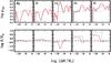 |
Fig. 2 Upper row: radiative accelerations for five atomic species, after 232 Myr of evolution in a model with a mass loss rate of 10-13 M⊙/yr (red curves) and in a model with turbulence (blue curves). The dotted lines represent gravity. Lower row: corresponding mass fraction in the model with mass loss and in that with turbulence. The dashed lines are the original values, which correspond to an original metallicity of Z0 = 0.01. |
The radiative accelerations of Mg, Si, Ca, Fe, and Ni are shown in the upper row of Fig. 2 at ~232 Myr, the approximate age of Sirius A, in both a model calculated with mass loss (red curves) and one calculated with turbulence (blues curves). The two are practically superposed for log ΔM/M∗ > −5 but differ significantly for many species closer to the surface (that is log ΔM/M∗ < −5). In the lower row, the corresponding internal concentrations for the model with mass loss and the one with turbulence are shown. When there is a difference between the grad’s for the two models, it is caused by saturation, as may be seen by comparing the abundances in the lower row. The X(Fe) and X(Ni) are larger in the model with turbulence for log ΔM/M∗ < −5 than in the model with mass loss; the reduction in the photon flux at the wavelengths where Fe and Ni absorb the most is by a larger factor when the abundance is higher, hence the grad’s are smaller in the model with turbulence. The large underabundance of Ca at log ΔM/M∗ ~ −7.5 in the wind model causes the larger grad(Ca) there, but the large underabundance is also caused by the maximum of grad(Ca) as discussed in Sect. 5.1.1 of Vick et al. (2010) to which the reader is referred for a detailed discussion of the interior wind solution. While the surface abundances of say Fe and Ni in the model with mass loss are within 0.3 dex of those in the model with turbulence, their interior mass fractions differ by a factor of about 5 for −7 < log ΔM/M∗ < −5.
Figures B.2 and B.1 contain results for all calculated species; they are shown in Appendix B.
4. Surface abundances
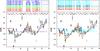 |
Fig. 3 Observed and predicted abundances on Sirius A as a function of Z, the atomic number, left in the model with turbulence calculated with an original metallicity of 0.009 for three slightly different values of turbulence and right in the model with mass loss with an original metallicity of 0.010 calculated with four different mass loss rates. The model name Z0.009_dY-0.02_mtb1.0 stands for a model calculated with Z0 = 0.009, ΔY = −0.02, and ΔM0 = 1.0 × 10⁻⁶ M⊙. The model name MassLoss_Z0.010W2E-13 stands for a model calculated with dM/dt = −2 × 10-13 M⊙/yr. All dotted lines represent models of about 200 Myr. |
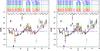 |
Fig. 4 Observed and predicted abundances on Sirius A as a function of Z, the atomic number, in the model with turbulence for two slightly different values of original metallicity, 0.010 and 0.011, and in the model with a mass loss rate of 10-13 M⊙/yr and a metallicity of 0.01 (see Fig. 3 for model labeling definitions). In the left panel, the two sets of observations are from Landstreet 2011: the black circles are from his observations while the pink triangles are an average over all recent observations (see the text). In the right panel, the averaged values are replaced by the actual data points of each observer as given in Table I of Landstreet (2011) where circles, Landstreet (2011); inverted open triangles, Lambert et al. (1982); inverted three-point stars, Lemke (1990); blue squares, Qiu et al. (2001); diamonds, Hill & Landstreet (1993); asterisks, Hui Bon Hoa et al. (1997); plus, Rentzsch-Holm (1997); upright open triangles, Holweger & Sturenburg (1993); pink squares, Sadakane & Ueta (1989). See the text for the explanation of the differences between the error bars in the right and left panels. |
Given the constraints imposed by age, Teff, L, and R, and that the mass is 2.1 M⊙, the original metallicity is fixed to Z0 = 0.010 ± 0.001 (see Sect. 2). More precisely, the luminosity (middle left hand panel of Fig. 1) implies that Z0 = 0.010 ± 0.001 and the radius then constrains the acceptable age to lie between 200 and 230 Myr (middle right hand panel). There only remains mass loss rates or mass mixed by turbulence that may be varied to define a range of predicted abundances that can then be compared with observations.
Evolutionary models were calculated for ΔM0 = 1.0, 1.4, and 2.1 × 10⁻⁶ M⊙ (see Eq. (3)) and for mass loss rates of 0.5, 0.7, 1.0, and 2.0 × 10⁻¹³ M⊙/yr. In Fig. 3, predictions from some of them are compared with observations from Col. 2 of Table 1 of Landstreet (2011). In Fig. 4, data from the other columns of his Table 1 are also used to present a picture of the uncertainties of the observations, as briefly discussed below.
In the left panel of Fig. 3, results are shown for the case Z0 = 0.009 at 200 Myr (dotted line segments) and at 220 Myr (solid line segments), which is the age interval over which all constraints are satisfied according to Fig. 1. In practice, even though shown for all cases, the dotted and solid segments are barely distinguishable and merely widen the dots. Note the assumed original composition at age 0.0 Myr in light blue on each panel of Figs. 3 and 4. As the mass mixed by turbulence is decreased from 2.1 to 1.0 × 10⁻⁶ M⊙, the surface abundance of elements supported by grad (e.g. most Fe peak elements) and the underabundance factor of sinking elements both increase. In the left panel of Fig. 4, similar results are shown for original metallicities of Z0 = 0.010 and 0.011 with ΔM0 = 1.4 × 10⁻⁶ M⊙. Within the range of original metallicities acceptable according to Sect. 2 (from Z0 = 0.009 to 0.011), the level of agreement between predicted surface abundances and observed ones does not change much although the Z0 = 0.010 case is slightly favored. Given the number of observed species, there is in practice little room for adjustment: as one may see from the left panel of Fig. 3, the Fe peak abundances are more consistent with the lower value of the mixed mass but the abundances of He, O, S and Ca are instead more consistent with the larger value.
Predictions for four mass loss rates and a metallicity of Z0 = 0.010 are shown in the right panel of Fig. 3. Only one metallicity is shown since the effects of changing metallicity over the acceptable range of Z0 = 0.009 to 0.011 are small as briefly mentioned above for the turbulence models. The iron peak elements would probably favor a mass loss rate of 0.5 × 10⁻¹³ M⊙/yr, but the lower mass species would then disagree more strongly with the predictions, and the most suitable compromise appears to be the 1.0 × 10⁻¹³ M⊙/yr case. The iron peak elements show approximately the same sensitivity to the mass loss range as to the mixed mass range illustrated in Fig. 3 but He, O and S are more sensitive to the mass loss rate4.
 |
Fig. 5 Color-coded interior concentrations for the same Z0 = 0.010 models as in Fig. 4 at ~233 Myr left in the model with turbulence and right in the model with mass loss. The radial coordinate is the radius and its scale is linear, but the logarithmic value of the mass coordinate above a number of points, log ΔM/M∗, is shown on the left of the horizontal black line. The concentration scale is given in the right insert. Small circles near the center of both models mark the central convection zone. While the surface abundances are very similar, as seen in Fig. 4, the interior concentrations are quite different between log ΔM/M∗ = −3 and the surface. |
In the left and right panels of Fig. 4, are shown the same three theoretical models (two calculated with turbulence and one with mass loss) compared to two different presentations of the results from Table 1 of Landstreet (2011). In the left panel, are shown both his determinations (his column labeled L11) and, as separate data points, his determinations averaged with those of the other observers he lists in his table, except for a few values he argues are erroneous or too uncertain to be worth including (his column labeled mean). The error bars are standard deviations of the observations listed in his table. These do not include contributions from the error bars of the various authors. The actual values of the different observers listed in his Table 1 are shown in the right panel of Fig. 4. The values that Landstreet excluded from his averages are not shown but all others are. One can argue that the differences in the abundance values determined by the various observers provide a better estimate of the uncertainty in the abundance determinations than the mean value with associated standard deviation shown in the left panel. Following a discussion with Landstreet (priv. comm.), the error bars for his points (from his column L11) were slightly increased for the right panel of Fig. 4 only. Thus, in all cases where, in the “L11” column of Table 1, he had 0.1, we increased this to 0.15 because this is closer to the actual dispersion found for dominant ions with many lines. Noting that there is some additional uncertainty (about 0.1 dex) because of the imprecise fundamental parameters and microturbulence, another 0.1 dex was added in quadrature to all sigmas, giving a minimum sigma of 0.18.
In the right panel of Fig. 4, we present our comparison between theory and observations. The agreement is not perfect for any value of turbulence or mass loss. The difference between the mass loss and turbulent models is very small for atomic species lighter than Cr and one may question whether abundances alone can really distinguish between the two given the error bars. Among the species included in our calculations, abundances were determined observationally for 17 atomic species and upper limits for 4. For the model Z0 = 0.010 with ΔM0 = 1.4 × 10⁻⁶ M⊙ one counts 8 species within 1σ and an additional 6 within 2σ. These numbers are respectively 8 and 7 for the Z0 = 0.011 model with the same turbulence. One counts respectively 8 and 5 for the Z0 = 0.010 mass loss model with a mass loss rate of 1.0 × 10⁻¹³ M⊙/yr. In addition, among the 4 upper limits, 3 are compatible with predictions. While the trend is right, the agreement is not so good for Ti, Cr, and Mn.
The interior concentrations in the two Z0 = 0.01 models of Fig. 4 are shown in Fig. 5. While the surface abundances are quite similar in the two, the interior concentrations are quite different for log ΔM/M∗ < −3 (see Sect. 3).
If one compares these results with Fig. 20 of Vick et al. (2010), one notes that the same mass loss rate of 1.0 × 10⁻¹³ M⊙/yr was found to lead to the prediction closest to the observed abundances. While the age assumed for Sirius is about the same in the two papers, the larger mass of the models used in Vick et al. (2010) causes them to be more evolved and, so, have a smaller gravity at a similar age. This is an important difference, when one compares two models with approximately the same Teff and thus the same grad. Another difference comes from the original Z0, which is 0.010 for the mass loss models of Fig. 4 of this paper, but 0.02 for those of Fig. 20 of Vick et al. (2010).
5. Conclusion
We have investigated what can be learned from the chemical composition of Sirius A. Using observationally determined stellar parameters for Sirius A we have first fixed an original metallicity and He mass fraction (Sect. 2). We have then predicted the expected surface abundances as a function of either a surface mass mixed by turbulence or a mass loss rate. Among the 17 abundances determined observationally, up to 15 can be predicted to within 2σ, and 3 of the 4 determined upper limits are satisfied. The three atomic species B, N, and Na show the strongest disagreement.
While the origin of the assumed turbulence has not been determined, it could be either shear induced by differential rotation (Talon et al. 2006) or be gravity waves (Talon & Charbonnel 1998). If the main competing process is mass loss, however, it has the great advantage that it has been previously observed (Bertin et al. 1995). The mass loss rate of 1.0 × 10⁻¹³ M⊙/yr that best reproduces abundance observations is slightly larger than the lower limit of 6 × 10-14 M⊙/yr determined from asymmetries of Mg II lines using the ST observations of these authors (see Eq. (1)). Their estimate based on corrected LTE, their Eq. (12), however, gives a mass loss rate between 5.0 × 10⁻¹² and 5.0 × 10⁻¹¹ M⊙/yr, which would lead to practically no surface abundance variations during evolution, in contradiction with the observed Sirius abundances (see Figs. 11 and 20 of Vick et al. 2010, for a calculation with 1.0 × 10⁻¹² M⊙/yr). Our results then vindicate the arguments presented above in Sect. 1 that support their estimate based on radiative ionization fraction. While by themselves, abundances do not favor mass loss or turbulence as the competing process, the agreement with the observationally determined mass loss rate favors mass loss.
While there probably still remains some uncertainties in the observationally determined abundances, the disagreement between observations and calculations indicates that there remain some weaknesses in the models. The first one may be related to the presence of Sirius B. Even though Sirius is quite a wide pair, it had been suggested by Richer et al. (2000) that the disagreement with the C and N observations could be caused by the transfer of material from the former primary. This was discussed by Landstreet (2011), who also suggested that it could simultaneously explain the difficulty with the B upper limit. Sodium could also be affected, just as it is affected in the globular cluster M4 (Marino et al. 2011). However, the extent of the mass transfer in Sirius remains uncertain.
Even if it is tempting to accept mass loss as the most important mechanism competing with diffusion in slowly rotating stars, it is also observed that abundance anomalies are much less important in rapidly rotating stars. Another mechanism linked to rotation must then be involved. Either rotation-driven turbulence (Talon et al. 2006) or meridional circulation (Charbonneau & Michaud 1991) could progressively reduce abundance anomalies as rotation increases. The weak dependence of abundance anomalies on the rotation rate could be due to its effect becoming larger than those of mass loss only as one approaches the 100 km s-1 limit of vsini (Abt 2000) for the Am star phenomenom.
In relation to Fig. 5, it was suggested in Sect. 4 that asterosismology tests could distinguish between mass loss and turbulence as the competing mechanism for slowly rotating stars. While detailed evolutionary calculations with meridional circulation have not yet been carried out, one expects that laminar meridional circulation would lead to internal metal distributions, in three dimensions, similar to those that mass loss leads to, in one dimension, since both are advective and not diffusive processes. This opens the possibility of distinguishing between meridional circulation and rotation-induced turbulence using asterosismology.
For simplicity, these calculations have been carried out with undifferentiated mass loss throughout Sirius A’s evolution, as seems appropriate for Am stars. However, a 2.1 M⊙ star begins its main-sequence at Teff ~ 10 500 K (see Fig. 1), where no H convection zone is present and which is probably within the HgMn domain. What then would the mass loss rate have been? The observation of Hg isotope anomalies on HgMn stars suggests that the mass loss would be differentiated (see Michaud et al. 1974; and Sect. 4 of Michaud & Richer 2008). How would this affect surface abundances during later evolutionary stages, such as reached by Sirius A?
Online material
Appendix A: Properties of models
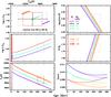 |
Fig. A.1 An HR diagram and the time evolution of Teff, L, log g, R, and Zsurf are shown. Observationally determined ± 1σ intervals are shown for L, Teff, g, and R. For Teff, the spectroscopically determined error bar is in black, while that determined using luminosity and radius is in red (see the text). Each model is color coded and identified in the figure. The adopted acceptable age range is from 200 to 250 Myr (see the text). In the HR diagram, only the part of the curves between 200 and 250 Myr is shown; see Fig. 1 for a more complete figure. All models were calculated with turbulence. |
Appendix B: Radiative accelerations and interior concentrations for all species
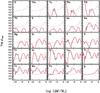 |
Fig. B.1 Radiative accelerations after 232 Myr evolution in a model with mass loss of 10-13 M⊙/yr (red curves) and in a model with turbulence with ΔM0 = 1.4 × 10⁻⁶ M⊙ (blue curves) for all calculated atomic species. The sharp mimima in the grad(Ti), grad(Cr), and grad(Mn) curves at log ΔM/M∗ ~ − 10 appear surprising but have been verified to be a systematic property of the OPAL atomic data. |
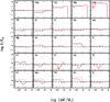 |
Fig. B.2 Mass fractions in the models with turbulence (blue curves) and mass loss (red curves). See the caption of Fig. B.1. |
This is slightly different from their Eq. (17), for which they had neglected the error bar given with their Eq. (7) but included an evaluation of the Mg II ionization based on a corrected LTE value coming from atmosphere models (Snijders & Lamers 1975) that do not seem appropriate for the wind region of interest here.
This 0.02 reduction of Y for a 0.01 reduction of Z is the same proportionality as used by VandenBerg et al. (2000) in building his Table 2. LiBeB were taken from the meteoretic values of Grevesse & Sauval (1998).
The values of D(He)0 actually used in this formula were always obtained – for programming convenience – from the simple analytical approximation D(He) = 3.3 × 10⁻¹⁵T2.5/ [4ρln(1 + 1.125 × 10⁻¹⁶T3/ρ)] (in cgs units) for He in trace amount in an ionized hydrogen plasma. These can differ significantly from the more accurate values used elsewhere in the code.
As the mass loss rate is reduced, the settling velocity becomes closer in magnitude to the wind velocity. This tends to amplify differences in the settling velocities that are caused, among other factors, by small mass differences. For instance, the abundance variation of 4He is a factor of 1.8 larger than that of 3He for the 0.5 × 10⁻¹³ M⊙/yr case but only a factor of 1.3 larger in the 10-13 M⊙/yr case (see the right panel of Fig. 3).
Acknowledgments
We thank Dr. John Landstreet for very kindly communicating to us his results ahead of publication and for useful discussions. We thank Dr. David Leckrone for a constructive criticism of the manuscript and useful suggestions that led to significant improvements. This research was partially supported at the Université de Montréal by NSERC. We thank the Réseau québécois de calcul de haute performance (RQCHP) for providing us with the computational resources required for this work.
References
- Abbott, D. C. 1982, ApJ, 259, 282 [NASA ADS] [CrossRef] [Google Scholar]
- Abt, H. A. 2000, ApJ, 544, 933 [NASA ADS] [CrossRef] [Google Scholar]
- Babel, J. 1995, A&A, 301, 823 [Google Scholar]
- Bertin, P., Lamers, H. J. G. L. M., Vidal-Madjar, A., Ferlet, R., & Lallement, R. 1995, A&A, 302, 899 [NASA ADS] [Google Scholar]
- Charbonneau, P., & Michaud, G. 1991, ApJ, 370, 693 [NASA ADS] [CrossRef] [Google Scholar]
- Grevesse, N., & Sauval, A. J. 1998, Space Sci. Rev., 85, 161 [NASA ADS] [CrossRef] [Google Scholar]
- Hill, G. M., & Landstreet, J. D. 1993, A&A, 276, 142 [NASA ADS] [Google Scholar]
- Holweger, H., & Sturenburg, S. 1993, in Peculiar versus Normal Phenomena in A-type and Related Stars, IAU Colloq. 138, ed. M. M. Dworetsky, F. Castelli, & R. Faraggiana, ASP Conf. Ser., 44, 356 [Google Scholar]
- Hui Bon Hoa, A., Burkhart, C., & Alecian, G. 1997, A&A, 323, 901 [NASA ADS] [Google Scholar]
- Iglesias, C. A., & Rogers, F. J. 1996, ApJ, 464, 943 [NASA ADS] [CrossRef] [Google Scholar]
- Kervella, P., Thévenin, F., Morel, P., Bordé, P., & Di Folco, E. 2003, A&A, 408, 681 [NASA ADS] [CrossRef] [EDP Sciences] [Google Scholar]
- Lambert, D. L., Roby, S. W., & Bell, R. A. 1982, ApJ, 254, 663 [NASA ADS] [CrossRef] [Google Scholar]
- Landstreet, J. D. 2011, A&A, 528, A132 [NASA ADS] [CrossRef] [EDP Sciences] [Google Scholar]
- Lemke, M. 1989, A&A, 225, 125 [Google Scholar]
- Lemke, M. 1990, A&A, 240, 331 [Google Scholar]
- Marino, A. F., Villanova, S., Milone, A. P., et al. 2011, ApJ, 730, L16 [NASA ADS] [CrossRef] [Google Scholar]
- Michaud, G., & Richer, J. 2008, Contributions of the Astronomical Observatory Skalnate Pleso, 38, 103 [NASA ADS] [Google Scholar]
- Michaud, G., Reeves, H., & Charland, Y. 1974, A&A, 37, 313 [NASA ADS] [Google Scholar]
- Michaud, G., Richer, J., & Richard, O. 2011, A&A, 529, A60 [NASA ADS] [CrossRef] [EDP Sciences] [Google Scholar]
- Pinsonneault, M. H., Kawaler, S. D., Sofia, S., & Demarque, P. 1989, ApJ, 338, 424 [NASA ADS] [CrossRef] [Google Scholar]
- Proffitt, C. R., & Michaud, G. 1991, ApJ, 380, 238 [NASA ADS] [CrossRef] [Google Scholar]
- Qiu, H. M., Zhao, G., Chen, Y. Q., & Li, Z. W. 2001, ApJ, 548, 953 [NASA ADS] [CrossRef] [Google Scholar]
- Rentzsch-Holm, I. 1997, A&A, 317, 178 [Google Scholar]
- Richer, J., Michaud, G., & Turcotte, S. 2000, ApJ, 529, 338 [NASA ADS] [CrossRef] [Google Scholar]
- Sadakane, K., & Ueta, M. 1989, PASJ, 41, 279 [NASA ADS] [Google Scholar]
- Snijders, M. A. J., & Lamers, H. J. G. L. M. 1975, A&A, 41, 245 [NASA ADS] [Google Scholar]
- Talon, S., & Charbonnel, C. 1998, A&A, 335, 959 [NASA ADS] [Google Scholar]
- Talon, S., & Charbonnel, C. 2005, A&A, 440, 981 [NASA ADS] [CrossRef] [EDP Sciences] [Google Scholar]
- Talon, S., Richard, O., & Michaud, G. 2006, ApJ, 645, 634 [NASA ADS] [CrossRef] [Google Scholar]
- Turcotte, S., Richer, J., Michaud, G., Iglesias, C., & Rogers, F. 1998, ApJ, 504, 539 [NASA ADS] [CrossRef] [Google Scholar]
- VandenBerg, D. A., Swenson, F. J., Rogers, F. J., Iglesias, C. A., & Alexander, D. R. 2000, ApJ, 532, 430 [NASA ADS] [CrossRef] [Google Scholar]
- Vick, M., Michaud, G., Richer, J., & Richard, O. 2010, A&A, 521, A62 [NASA ADS] [CrossRef] [EDP Sciences] [Google Scholar]
All Figures
|
Fig. 1 An HR diagram and the time evolution of Teff, L, log g, R, and Zsurf are shown. Observationally determined ± 1σ intervals are shown for L, Teff, g, and R. For Teff, the spectroscopically determined error bar is in black, while that determined using luminosity and radius is in red (see the text). Each model is color coded and identified on the figure. The adopted acceptable age range is from 200 to 250 Myr (see the text). In the HR diagram, the part of the curves between 200 and 250 Myr is solid; it is dotted outside that interval. All models were calculated with turbulence. Models with mass loss could not be distinguished, in the HR diagram, from those of the same original mass and composition calculated with turbulence. A subset of the curves is shown in Fig. A.1. |
| In the text | |
|
Fig. 2 Upper row: radiative accelerations for five atomic species, after 232 Myr of evolution in a model with a mass loss rate of 10-13 M⊙/yr (red curves) and in a model with turbulence (blue curves). The dotted lines represent gravity. Lower row: corresponding mass fraction in the model with mass loss and in that with turbulence. The dashed lines are the original values, which correspond to an original metallicity of Z0 = 0.01. |
| In the text | |
|
Fig. 3 Observed and predicted abundances on Sirius A as a function of Z, the atomic number, left in the model with turbulence calculated with an original metallicity of 0.009 for three slightly different values of turbulence and right in the model with mass loss with an original metallicity of 0.010 calculated with four different mass loss rates. The model name Z0.009_dY-0.02_mtb1.0 stands for a model calculated with Z0 = 0.009, ΔY = −0.02, and ΔM0 = 1.0 × 10⁻⁶ M⊙. The model name MassLoss_Z0.010W2E-13 stands for a model calculated with dM/dt = −2 × 10-13 M⊙/yr. All dotted lines represent models of about 200 Myr. |
| In the text | |
|
Fig. 4 Observed and predicted abundances on Sirius A as a function of Z, the atomic number, in the model with turbulence for two slightly different values of original metallicity, 0.010 and 0.011, and in the model with a mass loss rate of 10-13 M⊙/yr and a metallicity of 0.01 (see Fig. 3 for model labeling definitions). In the left panel, the two sets of observations are from Landstreet 2011: the black circles are from his observations while the pink triangles are an average over all recent observations (see the text). In the right panel, the averaged values are replaced by the actual data points of each observer as given in Table I of Landstreet (2011) where circles, Landstreet (2011); inverted open triangles, Lambert et al. (1982); inverted three-point stars, Lemke (1990); blue squares, Qiu et al. (2001); diamonds, Hill & Landstreet (1993); asterisks, Hui Bon Hoa et al. (1997); plus, Rentzsch-Holm (1997); upright open triangles, Holweger & Sturenburg (1993); pink squares, Sadakane & Ueta (1989). See the text for the explanation of the differences between the error bars in the right and left panels. |
| In the text | |
|
Fig. 5 Color-coded interior concentrations for the same Z0 = 0.010 models as in Fig. 4 at ~233 Myr left in the model with turbulence and right in the model with mass loss. The radial coordinate is the radius and its scale is linear, but the logarithmic value of the mass coordinate above a number of points, log ΔM/M∗, is shown on the left of the horizontal black line. The concentration scale is given in the right insert. Small circles near the center of both models mark the central convection zone. While the surface abundances are very similar, as seen in Fig. 4, the interior concentrations are quite different between log ΔM/M∗ = −3 and the surface. |
| In the text | |
|
Fig. A.1 An HR diagram and the time evolution of Teff, L, log g, R, and Zsurf are shown. Observationally determined ± 1σ intervals are shown for L, Teff, g, and R. For Teff, the spectroscopically determined error bar is in black, while that determined using luminosity and radius is in red (see the text). Each model is color coded and identified in the figure. The adopted acceptable age range is from 200 to 250 Myr (see the text). In the HR diagram, only the part of the curves between 200 and 250 Myr is shown; see Fig. 1 for a more complete figure. All models were calculated with turbulence. |
| In the text | |
|
Fig. B.1 Radiative accelerations after 232 Myr evolution in a model with mass loss of 10-13 M⊙/yr (red curves) and in a model with turbulence with ΔM0 = 1.4 × 10⁻⁶ M⊙ (blue curves) for all calculated atomic species. The sharp mimima in the grad(Ti), grad(Cr), and grad(Mn) curves at log ΔM/M∗ ~ − 10 appear surprising but have been verified to be a systematic property of the OPAL atomic data. |
| In the text | |
|
Fig. B.2 Mass fractions in the models with turbulence (blue curves) and mass loss (red curves). See the caption of Fig. B.1. |
| In the text | |
Current usage metrics show cumulative count of Article Views (full-text article views including HTML views, PDF and ePub downloads, according to the available data) and Abstracts Views on Vision4Press platform.
Data correspond to usage on the plateform after 2015. The current usage metrics is available 48-96 hours after online publication and is updated daily on week days.
Initial download of the metrics may take a while.