| Issue |
A&A
Volume 534, October 2011
|
|
|---|---|---|
| Article Number | A116 | |
| Number of page(s) | 8 | |
| Section | The Sun | |
| DOI | https://doi.org/10.1051/0004-6361/201116982 | |
| Published online | 18 October 2011 | |
Proton firehose instability in bi-Kappa distributed plasmas
1
Center for Plasma Astrophysics, Celestijnenlaan 200B,
3001
Leuven,
Belgium
e-mail: This email address is being protected from spambots. You need JavaScript enabled to view it.
2
Institut für Theoretische Physik, Lehrstuhl IV: Weltraum- und
Astrophysik, Ruhr-Universität Bochum, 44780
Bochum,
Germany
Received:
30
March
2011
Accepted:
21
June
2011
Abstract
Context. Protons or heavier ions with anisotropic velocity distributions and non-thermal departure from Maxwellian, are frequently reported in the magnetosphere and at different altitudes in the solar wind. These observations are sustained by an extended number of mechanisms of acceleration in any direction with respect to the interplanetary magnetic field. However, the observed anisotropy is not large and most probably constrained by the kinetic instabilities.
Aims. An excess of parallel kinetic energy, T∥/T⊥ > 1 (where ∥ and ⊥ denote directions relative to the background magnetic field) drives a proton firehose mode to grow, limiting any further increase in the anisotropy according to the observations. The effects of suprathermal populations on the principal characteristics of the proton firehose instability are investigated.
Methods. For low-collisional plasmas, the dispersion approach is based on the fundamental kinetic Vlasov-Maxwell equations. The anisotropy of plasma distributions including suprathermal populations is modeled by bi-Kappa functions, and the new dispersion relations are derived in terms of the modified plasma dispersion function (for Kappa distributions), and analytical approximations of this function.
Results. Growth rates of the proton firehose solutions and threshold conditions are provided in analytical forms for different plasma regimes. The proton firehose instability needs a larger anisotropy and a larger parameter β∥ to occur in a Kappa-distributed plasma. A precise numerical evaluation shows that the growth rates are, in general, lower and the wave frequency is only slightly affected, but the influence of suprathermal populations is essentially dependent on both the proton and electron anisotropies. Departures from the standard dispersion of a Maxwellian plasma can eventually be used to evaluate the presence of suprathermal populations in solar flares and the magnetosphere.
Key words: Sun: flares / plasmas / solar wind / instabilities / Sun: coronal mass ejections (CMEs)
© ESO, 2011
1. Introduction
Kinetic instabilities prevail in the solar wind (Cairns et al. 2000; Bale et al. 2009) as it is a dilute plasma that contains ample free energy, localized in flows, and a nonuniform heating (Marsch 2006; Bougeret & Pick 2007). In a poor-collisional plasma, these instabilities provide a plausible mechanism to prevent the development of excessive anisotropies and ensure a more fluid-like behavior (Hellinger et al. 2006; Stverak et al. 2008). Moreover, the electromagnetic wave turbulence leads to acceleration and pitch-angle scattering and diffusion, and must therefore play an important role in the evolution of plasma particles in the solar wind and the magnetosphere (Dröge 2003; Schlickeiser et al. 2010; Pierrard et al. 2011)
Measurements of the plasma parameters at high altitudes in the solar wind (≲ 1 AU) closely agree with theoretical and numerical predictions (Gary et al. 1976; Quest & Shapiro 1996; Gary et al. 1998; Hellinger & Matsumoto 2000; Matteini et al. 2006) showing that any increase in the parallel proton temperature is constrained by the proton firehose instability (PFHI) (Kasper et al. 2002; Hellinger et al. 2006; Bale et al. 2009). This instability is driven by an excess of the parallel kinetic energy, i.e. temperature Tp,∥ > Tp,⊥ or pressure p∥ > p⊥, and develops from a right-handed (RH) circularly polarized mode with a maximum growth rate at parallel propagation, i.e., k × B0 = 0. The mechanism that converts the kinetic energy of the protons and excites the firehose instability is essentially non-resonant, or fluid-like (Parker 1958; Pilipp & Völk 1971; Yoon 1995; Wang & Hau 2003). For a finite thermal spread, it has already been shown that resonant particles can also play an important role enhancing or suppressing the instability (Pilipp & Völk 1971; Gary et al. 1998), and shaping the proton distribution function to depart from the bi-Maxwellian form (Matteini et al. 2006). Resonant terms can, therefore, be considered whenever their contribution is expected to be significant.
Protons or heavier ions with suprathermal distributions have frequently been observed in the solar wind (Collier et al. 1996; Chotoo et al. 2000), the magnetosphere (Gloeckler & Hamilton 1987), or further in the heliosphere towards the termination shock (Decker et al. 2005; Fisk & Gloeckler 2007). There is abundant observational evidence indicating that particle energization and the occurrence of suprathermal populations are correlated with an enhanced activity of the waves and instabilities in space plasma. A brief description of these mechanisms of acceleration can be found in the review (referred to in Sect. 3) by Pierrard & Lazar (2010). Populations with suprathermal high-energy tails are most accurately modeled by the family of Kappa functions (Vasyliunas 1968; Summers & Thorne 1991), and may exhibit different wave dispersion and stability properties from a Maxwellian (Pierrard & Lazar 2010). Electrons with a surplus of parallel kinetic energy, Te,∥ > Te,⊥, initiate the electron firehose instability (EFHI) of the low-frequency left-handed (LH) circularly polarized modes propagating parallel to the magnetic field. Modeling the anisotropy of suprathermal electrons with a bi-Kappa distribution, Lazar & Poedts (2009) demonstrated that, compared to a bi-Mawellian, the threshold of the EFHI increases, the maximum growth rates are slightly diminished, and the instability extends to large wave numbers.
The PFHI is also a low-frequency growing mode but with a RH circular polarization, and is driven by the non-resonant protons with Tp,∥ > Tp,⊥. Under the usual convention, protons resonate more easily with LH modes driving a proton cyclotron instability if Tp,∥ < Tp,⊥. However, for an intense magnetization in low-β plasmas, the same resonant protons can also cause the instability of the RH modes to grow. In this case, the growth rates are usually much lower than the proton gyrofrequency, but they can increase (by a few orders of magnitude), approaching the proton gyrofrequency as the abundance of the suprathermal protons increases (Xue et al. 1993; Dasso et al. 2003). In addition, we consider large-β plasmas where deviations of the protons from an isotropic Maxwellian equilibrium can easily develop and drive the PFHI.
2. Parallel RH transverse modes in bi-Kappa plasmas
We start from the general dispersion relation of the transverse modes propagating
along the regular magnetic field with a RH circular polarization, e.g.,
Eq. (2) from Lazar & Poedts (2009), hereafter
called Paper I, ![Mathematical equation: \begin{eqnarray} 1 - {k^2c^2 \over \omega^2} && + {\pi \over \omega^2} \sum_a \omm_{{\rm p},a}^2 \int_{-\infty}^{\infty} \, {{\rm d}v_{\parallel} \over \omm - k v_{\parallel} + \Omega_a} \notag \\ \label{e1}\times && \int_0^{\infty} \, {\rm d}v_{\perp} v_{\perp}^2 \left[(\omm - k v_{\parallel}) {\partial F_{a,\kappa} \over \partial v_{\perp}} + k v_{\perp} {\partial F_{a,\kappa} \over \partial v_{\parallel}} \right] = 0, \end{eqnarray}](/articles/aa/full_html/2011/10/aa16982-11/aa16982-11-eq13.png) (1)where
ω and k denote the frequency and the wave number of the
plasma modes, respectively, c is the speed of light in a vacuum,
Ωa = qaB0/(mac)
is the (non-relativistic) gyrofrequency, and
ωp,a = (4πnae2/ma)1/2
is the plasma frequency for the particles of species a. We use polar
coordinates in the particle velocity space
(1)where
ω and k denote the frequency and the wave number of the
plasma modes, respectively, c is the speed of light in a vacuum,
Ωa = qaB0/(mac)
is the (non-relativistic) gyrofrequency, and
ωp,a = (4πnae2/ma)1/2
is the plasma frequency for the particles of species a. We use polar
coordinates in the particle velocity space  (2)The initial unperturbed
plasma anisotropy is modeled with a bi-Kappa velocity distribution function of plasma
particles
(2)The initial unperturbed
plasma anisotropy is modeled with a bi-Kappa velocity distribution function of plasma
particles ![Mathematical equation: \begin{equation} F_{\kappa} = {1 \over \pi^{3/2} \theta_{\perp}^2 \theta_{\parallel}} \, {\Gamma (\kappa + 1) \over \kappa^{3/2} \Gamma(\kappa -1/2)} \, \Biggl[1 + {v_{\parallel}^2 \over \kappa \theta_{\parallel}^2} + {v_{\perp}^2 \over \kappa \theta_{\perp}^2}\Biggr]^{-\kappa -1} \label{e3}, \end{equation}](/articles/aa/full_html/2011/10/aa16982-11/aa16982-11-eq21.png) (3)which is normalized by
(3)which is normalized by
 . Here,
  (4)with
  (5)and
  (6)denote the
perpendicular and parallel thermal velocities, respectively. The bi-Kappa distribution
function given in Eq. (4) was introduced by
Summers & Thorne (1991) to describe
anisotropies of suprathermal populations, and it approaches a bi-Maxwellian as the spectral
index κ (<3/2) reaches very
large values κ → ∞.
(6)denote the
perpendicular and parallel thermal velocities, respectively. The bi-Kappa distribution
function given in Eq. (4) was introduced by
Summers & Thorne (1991) to describe
anisotropies of suprathermal populations, and it approaches a bi-Maxwellian as the spectral
index κ (<3/2) reaches very
large values κ → ∞.
Now we insert the distribution function in Eq. (3) into Eq. (1) and obtain the
general dispersion relation of the RH transverse modes in a bi-Kappa distributed plasma
![Mathematical equation: \begin{equation} 1- {k^2c^2 \over \omega^2} + \sum_a {\omega_{{\rm p},a}^2 \over \omega^2} \left\{ {\omega \over k \theta_{a, \parallel}}\, Z^0_{\kappa} (g_a) - A_a \, \left[1+ g_a Z^0_{\kappa} (g_a)\right] \right\} = 0. \label{e7} \end{equation}](/articles/aa/full_html/2011/10/aa16982-11/aa16982-11-eq30.png) (7)We use the modified
plasma dispersion function (Lazar et al. 2008a)
(7)We use the modified
plasma dispersion function (Lazar et al. 2008a)
 (8)with the argument
(a = e,p)
(8)with the argument
(a = e,p)  (9)and the temperature
anisotropy
(9)and the temperature
anisotropy  (10)In the limit of very large
values of κ → ∞, the modified plasma dispersion function given in Eq.
(8) converges to the standard dispersion
function of Fried & Conte (1961), and the
dispersion relation in Eq. (7) agrees exactly
with the dispersion relation derived for a Maxwellian plasma (Gary 1993).
(10)In the limit of very large
values of κ → ∞, the modified plasma dispersion function given in Eq.
(8) converges to the standard dispersion
function of Fried & Conte (1961), and the
dispersion relation in Eq. (7) agrees exactly
with the dispersion relation derived for a Maxwellian plasma (Gary 1993).
The newly modified dispersion function  was introduced by Lazar et al.
(2008a) to simplify the description of the
dispersion properties of the transverse modes and instabilities in Kappa distributed
plasmas. This function relates to the modified dispersion function
Zκ introduced by Summers & Thorne
(1991)
was introduced by Lazar et al.
(2008a) to simplify the description of the
dispersion properties of the transverse modes and instabilities in Kappa distributed
plasmas. This function relates to the modified dispersion function
Zκ introduced by Summers & Thorne
(1991)  (11)We simply use the small and
large argument expansions of Zκ (Summers
& Thorne 1991) to find for
(11)We simply use the small and
large argument expansions of Zκ (Summers
& Thorne 1991) to find for

 (12)
(12) (13)Each
of the approximative forms given in Eqs. (12) and (13) of the modified
dispersion function in Eq. (8) contains a
principal part with an important contribution from the non-resonant particles, and an
imaginary part given by the analytical continuation for the resonant particles with
velocities satisfying cyclotron resonance conditions (of the first dominant order), i.e.,
|ga| ≃ 1,
a = e,p. Because the mechanism that excites the firehose
instability is essentially non-resonant, we can describe the EFHI/PFHI only by considering a
finite non-resonant contribution of the electrons/protons in the analytical approximations.
(13)Each
of the approximative forms given in Eqs. (12) and (13) of the modified
dispersion function in Eq. (8) contains a
principal part with an important contribution from the non-resonant particles, and an
imaginary part given by the analytical continuation for the resonant particles with
velocities satisfying cyclotron resonance conditions (of the first dominant order), i.e.,
|ga| ≃ 1,
a = e,p. Because the mechanism that excites the firehose
instability is essentially non-resonant, we can describe the EFHI/PFHI only by considering a
finite non-resonant contribution of the electrons/protons in the analytical approximations.
We can explicitly characterize the conditions for large or small arguments of
 by restricting
ourselves to the lowest frequencies,
ωr < Ωp ≪ |Ωe|,
corresponding to modes excited by the proton firehose instability, and further simplifying
by considering two distinct cases:
by restricting
ourselves to the lowest frequencies,
ωr < Ωp ≪ |Ωe|,
corresponding to modes excited by the proton firehose instability, and further simplifying
by considering two distinct cases:
-
(a)
ωi < ωr (<Ωp ≪ |Ωe|) when |ge| ≷ 1 implies that kc/ωp,p ≶ (1/ακe) [mp/(meβe,∥)] 1/2, and |gp| ≷ 1 implies
 . In the limit of a
small ωr < Ωp, both
arguments are large, |ge| > 1 and
|gp| > 1, only for small wave numbers
. In the limit of a
small ωr < Ωp, both
arguments are large, |ge| > 1 and
|gp| > 1, only for small wave numbers
 .
Here, we introduced
.
Here, we introduced  ,
a = e,p;
,
a = e,p; -
(b)
ωr < ωi (<Ωp ≪ |Ωe|), when |ge| ≷ 1 implies the same kc/ωp,p ≶ (1/ακe) [mp/(meβe,∥)] 1/2, and |gp| ≷ 1 implies
![Mathematical equation: \hbox{$\omega_i /\Omega_{\rm p} \gtrless [(kc/\omega_{\rm p,p})^2 \alpha_{\kappa_{\rm p}}^2 \beta_{\rm p, \parallel}- 1]^{1/2}$}](/articles/aa/full_html/2011/10/aa16982-11/aa16982-11-eq60.png) . In
the limit of a small
ωi < Ωp, both
arguments are large, |ge| > 1 and
|gp| > 1, only for small wave numbers
. In
the limit of a small
ωi < Ωp, both
arguments are large, |ge| > 1 and
|gp| > 1, only for small wave numbers
The spectral domains where the approximations given in Eqs. (12) and (13) apply are displayed in Fig. 1a and b, in a dispersion frequency versus wave number diagram. Four regions are delimited by the resonance curves shown with dashed lines for protons and dotted lines for electrons: region R1 for |gp,e| > 1, region R2 for |ge| > 1 and |gp| < 1, region R3 for |ge,p| < 1, and, finally, region R4 for |ge| < 1 and |gp| > 1.
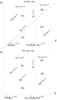 |
Fig. 1 Spectral domains R1–R4, where the approximations given in Eqs. (12) and (13) of the modified plasma dispersion function (8) can be used. For a dominance of suprathermal populations, indices κa → 1/2, and ακa → 0 increasing (meακeβe,∥/mp)−1/2 and (ακpβp,∥)−1/2 to very large values, and also enlarging the area where the arguments |ga| > 1 are large enough to apply the approximation in Eq. (13) for both species a = e,p, (Wr,i = ωr,i/Ωp, K = kc/ωp,p). |
The suprathermal populations are in general described by small values of the index
κ → 3/2 in the distribution function in Eq. (3). In this case,
ακa → 0 also
becomes very small causing the cutoffs of the resonance conditions
 and
and
 to reach very
large values. The region R1, where
|ga| > 1 for both
species a = e,p, can extend considerably to dominate the
other regions, where the arguments are smaller
(| ga| < 1). This
is the first important result of the present paper proving that in Kappa-distributed
plasmas, the arguments of the modified dispersion function become sufficiently large,
|ga| > 1, for a
large variety of plasma parameters, wave numbers, and frequencies, and that the
approximation derived in Eq. (13) enables a
simple analytical description of the unstable modes.
to reach very
large values. The region R1, where
|ga| > 1 for both
species a = e,p, can extend considerably to dominate the
other regions, where the arguments are smaller
(| ga| < 1). This
is the first important result of the present paper proving that in Kappa-distributed
plasmas, the arguments of the modified dispersion function become sufficiently large,
|ga| > 1, for a
large variety of plasma parameters, wave numbers, and frequencies, and that the
approximation derived in Eq. (13) enables a
simple analytical description of the unstable modes.
3. Proton firehose instability
Additional analytical derivations of the dispersion Eq. (7) can be easily undertaken to provide a detailed characterization of the
PFHI for specific plasma regimes. Thus, it is obvious to consider either the limit of small
temperatures (or small wave-numbers) when the argument of
 is large enough
(| ga| ≫ 1) for the approximation in
Eq. (13) to be applicable, or the opposite
limit of large temperatures (or large wave-numbers) when the argument becomes small
(| ga| ≪ 1) and the approximation in
Eq. (12) applies.
is large enough
(| ga| ≫ 1) for the approximation in
Eq. (13) to be applicable, or the opposite
limit of large temperatures (or large wave-numbers) when the argument becomes small
(| ga| ≪ 1) and the approximation in
Eq. (12) applies.
3.1. Cold fluid-like plasma (small wave numbers)
In this limit, both arguments are supposed to be very large, i.e.
|ga| ≫ 1 (with
a = e,p), and if we neglect the contribution of
resonant particles, the modified plasma dispersion function in the approximative form
given in Eq. (13) does not depend
explicitly on the spectral index κ (cf. Paper I), and the dispersion
relation (7) reduces to ![Mathematical equation: \begin{equation} {\omega^2 \over \Omega_{\rm p}^2} = {k^2c^2 \over \omega_{\rm p,p}^2} \left[1- {A_{\rm e} \over 2} \alpha_{\kappa_{\rm e}}^2 \beta_{{\rm e},\parallel} -{A_{\rm p} \over 2} \alpha_{\kappa_{\rm p}}^2 \beta_{{\rm p},\parallel}\right]. \label{e14} \end{equation}](/articles/aa/full_html/2011/10/aa16982-11/aa16982-11-eq82.png) (14)We have assumed that for
small wave numbers (real or imaginary) the frequencies are also sufficiently small,
ω2 ≪ k2c2
and ω ≪ Ωp ≪ |Ωe|. With
βe,∥ = (Te,∥/Tp,∥)βp,∥,
we simply find that in the limit of very large κ → ∞ (when
ακ → 1), the dispersion relation in
Eq. (14) agrees exactly with that
derived by Pilipp & Völk (1971, see
Eq. (3.3)) for a bi-Maxwellian plasma.
(14)We have assumed that for
small wave numbers (real or imaginary) the frequencies are also sufficiently small,
ω2 ≪ k2c2
and ω ≪ Ωp ≪ |Ωe|. With
βe,∥ = (Te,∥/Tp,∥)βp,∥,
we simply find that in the limit of very large κ → ∞ (when
ακ → 1), the dispersion relation in
Eq. (14) agrees exactly with that
derived by Pilipp & Völk (1971, see
Eq. (3.3)) for a bi-Maxwellian plasma.
An instability is expected to occur for  (15)i.e. when the dispersion
relation in Eq. (14) admits purely growing
solutions. This is the threshold condition of the firehose instability in the limit of
small wave numbers or a sufficiently cold, fluid-like plasma model. In this limit, the two
branches of LH and RH modes overlap, both being described by the same dispersion relation
given in Eq. (14) and the same threshold
condition in Eq. (15), and where the
non-resonant character of this instability is most clearly revealed by cumulating the
effects of both anisotropic components, electrons, and ions. Otherwise, if an instability
is resonantly growing because of the kinetic anisotropies of the plasma particles (see,
for instance, the cyclotron instabilities), the resonant enhancing effects from both
species cannot cumulate. Parker (1958) demonstrated
for the first time the existence of the firehose instability by considering a
(one-component) fluid model of anisotropic plasma with an excess of pressure parallel to
the magnetization field, and neglecting any resonances with plasma particles.
(15)i.e. when the dispersion
relation in Eq. (14) admits purely growing
solutions. This is the threshold condition of the firehose instability in the limit of
small wave numbers or a sufficiently cold, fluid-like plasma model. In this limit, the two
branches of LH and RH modes overlap, both being described by the same dispersion relation
given in Eq. (14) and the same threshold
condition in Eq. (15), and where the
non-resonant character of this instability is most clearly revealed by cumulating the
effects of both anisotropic components, electrons, and ions. Otherwise, if an instability
is resonantly growing because of the kinetic anisotropies of the plasma particles (see,
for instance, the cyclotron instabilities), the resonant enhancing effects from both
species cannot cumulate. Parker (1958) demonstrated
for the first time the existence of the firehose instability by considering a
(one-component) fluid model of anisotropic plasma with an excess of pressure parallel to
the magnetization field, and neglecting any resonances with plasma particles.
However, minimizing the role of collisions and assuming electrons and ions distributed after power laws of bi-Kappa type, here we find that both the growth rate and the threshold condition are sensitive to the shape of the distribution function exhibiting a strong dependence on the spectral index κ. The standard fluid-like model of the firehose instability is, therefore, recovered only in the Maxwellian limit of κ → ∞, when the plasma must be collisional and less tenuous. The growth rates are displayed in Fig. 2 for different values of the κ index, the temperature contrast, Te,∥/Tp,∥, and the plasma-β parameter.
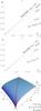 |
Fig. 2 Growth rates of the firehose instability as provided by Eq. (14) for κe = 2, κp = 3 (dotted line), κe,p = 4 (dashed line), κe,p → ∞ (solid line), and plasma parameters: Te,∥/Te,⊥ = Tp,∥/Tp,⊥ = 4, a) Te,∥/Tp,∥ = 3, βe,∥ = 18; and b) Te,∥/Tp,∥ = 2, βe,∥ = 8. For a given wave-number value K = 0.03, the growth rate variation with κe and κp is shown in panel c). (Wi = ωi/Ωp, K = kc/ωp,p). |
When we compare the contributions of each species, electrons and protons, we find that
the mass contrast
me/mp (or
 )
does not intervene (minimizing the contribution of the protons). It is, however, the
temperature contrast
Te,∥/Tp,∥
(<1, in the solar wind often in the favor of electrons) that
can lower the effect of protons, e.g., through
βp,∥ = (Tp,∥/Te,∥)βe, ∥ < βe,∥.
However, an important observation is that, in this limit (small wave-numbers), the effects
of both species, electrons and protons, are diminished in the presence of suprathermal
populations (small values of κe,p).
)
does not intervene (minimizing the contribution of the protons). It is, however, the
temperature contrast
Te,∥/Tp,∥
(<1, in the solar wind often in the favor of electrons) that
can lower the effect of protons, e.g., through
βp,∥ = (Tp,∥/Te,∥)βe, ∥ < βe,∥.
However, an important observation is that, in this limit (small wave-numbers), the effects
of both species, electrons and protons, are diminished in the presence of suprathermal
populations (small values of κe,p).
If the electrons are isotropic, i.e. Ae = 0, from the general
condition in Eq. (15) we find the
threshold condition for the PFHI  (16)where
 must be
sufficiently large. Alternatively, for isotropic protons, we substitute
Ap = 0 in Eq. (15) and find the threshold condition for the EFHI
must be
sufficiently large. Alternatively, for isotropic protons, we substitute
Ap = 0 in Eq. (15) and find the threshold condition for the EFHI  (17)assuming this time a
sufficiently large
(17)assuming this time a
sufficiently large  (for
instance, Eq. (5) provides
(for
instance, Eq. (5) provides
 for
κ = 2, and
for
κ = 2, and  for
κ = 4). We note that the reproduction of Eq. (17) here corrects a typographical error in
Paper I, Eq. (22), where the threshold condition for the EFHI was derived for the first
time. Both of these conditions in Eqs. (16) and (17) illustrate the need
for a larger kinetic anisotropy and a larger β∥ to produce
the instability in plasma with suprathermal populations. For comparison, the threshold
conditions for a Maxwellian plasma (κ → ∞) and different
low-κ plasmas are displayed in Fig. 3. We also note that in Fig. 2b no
instability grows for small values of κe = 1.8 and
κp = 2 because, for the given values of the plasma
parameters, the instability condition imposes a minimum limit value for the spectral index
κ (see Eq. (23) in Paper I).
for
κ = 4). We note that the reproduction of Eq. (17) here corrects a typographical error in
Paper I, Eq. (22), where the threshold condition for the EFHI was derived for the first
time. Both of these conditions in Eqs. (16) and (17) illustrate the need
for a larger kinetic anisotropy and a larger β∥ to produce
the instability in plasma with suprathermal populations. For comparison, the threshold
conditions for a Maxwellian plasma (κ → ∞) and different
low-κ plasmas are displayed in Fig. 3. We also note that in Fig. 2b no
instability grows for small values of κe = 1.8 and
κp = 2 because, for the given values of the plasma
parameters, the instability condition imposes a minimum limit value for the spectral index
κ (see Eq. (23) in Paper I).
When both species are anisotropic, i.e.
Ae,p ≠ 0, and exhibit suprathermal tails of
different shapes, (κe ≠ κp), the
general condition in Eq. (15) can be
rewritten in the same form as  (18)assuming this time a
sufficiently large
(18)assuming this time a
sufficiently large  .
.
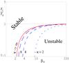 |
Fig. 3 Threshold conditions for the EFHI (or the PFHI) as provided by Eq. (16) (or in Eq. (17)) for different
values κ. The instability occurs below the threshold lines for
|

3.2. Hot electrons – isotropic distribution, Ae = 0
Considering a plasma with anisotropic protons, Tp,∥ > Tp,⊥, and isotropic electrons, Te,⊥ = Te,∥, the dispersion relation in Eq. (7) simplifies to
![Mathematical equation: \begin{eqnarray} && 1- {k^2c^2 \over \omega^2} + {\omega_{\rm p,p}^2 \over \omega^2} \left\{ {\omega \over k \theta_{{\rm p}, \parallel}}\, Z^0_{\kappa} (g_{\rm p}) - A_{\rm p} \, \left[1+ g_{\rm p} Z^0_{\kappa} (g_{\rm p})\right] \right\} \nonumber \\ \label{e19}&& \qquad \qquad+ {\omega_{\rm p,e}^2 \over \omega^2} \, {\omega \over k \theta_{{\rm e}, \parallel}}\, Z^0_{\kappa} (g_{\rm e}) = 0. \end{eqnarray}](/articles/aa/full_html/2011/10/aa16982-11/aa16982-11-eq133.png) (19)For
Maxwellian distributions with the same assumption of anisotropic protons and isotropic
electrons, the dispersion relation in Eq. (19) transforms, in the limit of κ → ∞, to
(19)For
Maxwellian distributions with the same assumption of anisotropic protons and isotropic
electrons, the dispersion relation in Eq. (19) transforms, in the limit of κ → ∞, to ![Mathematical equation: \begin{eqnarray} &&1- {k^2c^2 \over \omega^2} + {\omega_{\rm p,p}^2 \over \omega^2} \left\{ {\omega \over k v_{T_{{\rm p}, \parallel}}}\, Z(f_{\rm p}) - A_{\rm p} \, \left[1+ f_{\rm p} Z (f_{\rm p})\right] \right\} \nonumber \\ \label{e20} && \qquad \qquad\qquad\qquad + {\omega_{\rm p,e}^2 \over \omega^2} \, {\omega \over k v_{T_{{\rm e}, \parallel}}}\,Z (f_{\rm e}) = 0, \end{eqnarray}](/articles/aa/full_html/2011/10/aa16982-11/aa16982-11-eq134.png) (20)where
Z(f) is the standard plasma dispersion function (Fried
& Conte 1961) with the argument
(20)where
Z(f) is the standard plasma dispersion function (Fried
& Conte 1961) with the argument
 (21)If protons are still
assumed to be cold (and non-resonant), the argument in Eq. (9) of the plasma dispersion function will be large,
|gp| > 1. Here, we assume that
the electrons are hot so that the argument is
|ge| < 1, and they can resonate
with RH modes. (The non-resonant effects of the electrons are discussed in the other
sections and in Paper I). Limiting to the first order approximation of the modified plasma
dispersion function in Eqs. (12)
and (13), we obtain from Eq. (19)
(21)If protons are still
assumed to be cold (and non-resonant), the argument in Eq. (9) of the plasma dispersion function will be large,
|gp| > 1. Here, we assume that
the electrons are hot so that the argument is
|ge| < 1, and they can resonate
with RH modes. (The non-resonant effects of the electrons are discussed in the other
sections and in Paper I). Limiting to the first order approximation of the modified plasma
dispersion function in Eqs. (12)
and (13), we obtain from Eq. (19)  (22)where from
Eq. (12)
(22)where from
Eq. (12)  (23)Assuming
ω2 ≪ k2c2
and ω < Ωp the dispersion Eq. (22) reduces further to
(23)Assuming
ω2 ≪ k2c2
and ω < Ωp the dispersion Eq. (22) reduces further to  (24)which admits
unstable solutions of frequency
(24)which admits
unstable solutions of frequency  (25)and
growth rate
(25)and
growth rate  (26)when the same threshold
condition in Eq. (16) for the existence of
the PFHI is fulfilled.
(26)when the same threshold
condition in Eq. (16) for the existence of
the PFHI is fulfilled.
3.3. Hot electrons – anisotropic distribution, Ae ≠ 0
Two distinct cases are found here. First, if the electrons are anisotropic with a finite
but sufficiently small anisotropy to describe an excess of parallel or perpendicular
temperature,
0 < |Ae| < 1,
the instability occurs for the same condition in Eq. (16) and has the same growth rate in Eq. (26), but only the frequency changes to  (27)Second, if the
electron anisotropy is larger,
Te,∥ ≫ Te,⊥
but still in the limit of Ae ≲ 1, or if it is provided by a
surplus of perpendicular temperature,
Te,∥ ≪ Te,⊥
(Ae < 0), the wave solution will be
described (in the same limit of a small
ω < Ωp) by the real frequency
(27)Second, if the
electron anisotropy is larger,
Te,∥ ≫ Te,⊥
but still in the limit of Ae ≲ 1, or if it is provided by a
surplus of perpendicular temperature,
Te,∥ ≪ Te,⊥
(Ae < 0), the wave solution will be
described (in the same limit of a small
ω < Ωp) by the real frequency
 (28)and the imaginary
frequency
(28)and the imaginary
frequency 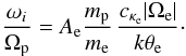 (29)The instability occurs
only for Ae > 0, otherwise the wave is
damped by the resonant electrons with
Te,⊥ ≫ Te,∥
(Ae < 0). As expected in this case,
if the instability occurs, it is exclusively driven by electrons (with a large excess of
the parallel temperature,
Te,⊥ ≪ Te,∥),
and it can change into an EFHI mode if the Ap is small enough
to switch the wave polarization, i.e. the sign of the wave frequency in Eq. (28). Thus, Eq. (29) describes analytically the negative-slope branch of the EFHI
growth rate displayed in Paper I, Fig. 1b: after a maximum at the saturation, the growth
rate decreases and does not vanish completely, but decreases asymptotically to zero.
(29)The instability occurs
only for Ae > 0, otherwise the wave is
damped by the resonant electrons with
Te,⊥ ≫ Te,∥
(Ae < 0). As expected in this case,
if the instability occurs, it is exclusively driven by electrons (with a large excess of
the parallel temperature,
Te,⊥ ≪ Te,∥),
and it can change into an EFHI mode if the Ap is small enough
to switch the wave polarization, i.e. the sign of the wave frequency in Eq. (28). Thus, Eq. (29) describes analytically the negative-slope branch of the EFHI
growth rate displayed in Paper I, Fig. 1b: after a maximum at the saturation, the growth
rate decreases and does not vanish completely, but decreases asymptotically to zero.
The instability of the RH modes can also be enhanced by the resonant protons (i.e. with a contribution from the imaginary residual part of the approximations in Eqs. (12) or (13)) producing ion (proton) cyclotron modes (Xue et al. 1993; Dasso et al. 2003), but this is possible only in small-β plasmas, and is not considered here.
3.4. Hot plasma (large wave numbers)
If both components, electrons and protons, are sufficiently hot, both arguments are small enough, i.e. |ge,p| ≪ 1 (region R3 in Fig. 1), and we use the approximation given in Eq. (12) for the modified plasma dispersion function. Keeping only the principal part in Eq. (12), we found no instability driven by the non-resonant particles. Some possible contribution from the resonant electrons in this case, is irrelevant for the firehose instability. The conclusion is that in this limit, the number of the non-resonant protons is not large enough to produce an instability of the firehose type. For electrons colder than protons, which is not the case in the solar wind plasma, the RH mode is damped (ωi < 0).
4. The exact numerical solutions of Eq. (7)
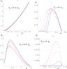 |
Fig. 4 The exact numerical solutions, the real frequency a) and the growth rate b), c), d) for the PFHI as provided by Eq. (7) for κp = 3 (dotted line), κp = 4 (dashed line), κp = 8 (long-dashed line), and κp → ∞ (solid line), and typical solar wind plasma parameters Te,∥/Tp,∥ = 2, βe,∥ = 8, (βp,∥ = 4), Te,⊥ = Te,∥ ≃ 106 K and different values of the proton anisotropy Tp,⊥/Tp,∥ = 0.25 a), b), 0.6 c), 0.8 d). Electrons are assumed to be isotropic and Maxwellian (κe → ∞). (Wr = ωr/Ωp, Wi = ωi/Ωp, K = kc/ωp,p). |
In Figs. 4–6 we plot the exact numerical solutions of Eq. (7), the real frequency Wr = ωr/Ωp, and the growth rate Wi = ωi/Ωp, and examine the influence that the Kappa index value can have on the evolution of the PFHI in different plasma regimes. Values of the plasma parameters including temperature anisotropy, are chosen from the in-situ measurements of the solar wind missions.
The three distinct cases displayed in Fig. 4 correspond to different proton anisotropies Tp,⊥/Tp,∥ = 0.25 (in panels a and b), 0.6 (c), 0.8 (d). The electrons are assumed to be isotropic (Ae = 0), and Maxwellian (κe → ∞). For comparison, the growth rates are calculated for different values of the spectral index, and their evolution depends markedly on the value of the proton anisotropy. At large anisotropies (panel b), the growth rate increases with κp reaching its maximum for Maxwellian (κp → ∞), but this tendency is restrained by decreasing the anisotropy, and for small anisotropies the growth rates show an opposite trend of variation, decreasing with κp index. If the instability suppression for small values of κp was anticipated by the more stringent threshold conditions found in Eq. (16) (and displayed in Fig. 3), the enhancement of the instability in the presence of Kappa populations with small anisotropies was unexpected. This new evolution seems to correspond to different threshold conditions that can eventually be obtained for an argument of the plasma dispersion function close to unity (| g| ~ 1). However, in the observations there is no constraint for such small anisotropies, and they are probably irrelevant. The real (oscillatory) frequency (panel a) does not change significantly with κp index in the range of unstable wave numbers. Comparing to the growth rates of the EFHI in Paper I, the maxima reached by the growth rate of the PFHI are in general lower. This also remains true for larger proton anisotropies, e.g. Tp,∥/Tp,⊥ = 20, similar to that used for electrons in Paper I. However, when assuming both components, electrons and protons, to be anisotropic, the evolution of the PFHI changes significantly.
Thus, an excess of the electron temperature perpendicular to the magnetic field, Te,⊥/Te,∥ > 1, is expected to enhance the RH polarized mode. This indeed happens, as shown in Fig. 5, but only for large wave numbers when the instability turns into the whistler instability, which is driven by electrons and is, in general, inhibited by the Kappa distributions (Lazar et al. 2008b). At small wave numbers, the PFHI is suppressed by the same anisotropy of electrons, and both the growth rate and the unstable wave numbers interval are reduced. In Kappa distributed plasmas, growth rates are further reduced (at small values of the κ index) if the electron anisotropy is sufficiently small (Fig. 5a). However, for a somewhat larger anisotropy, e.g., Te,⊥/Te,∥ = 1.5 (Fig. 5b), the evolution with κ changes again and the instability is enhanced at small values of κ. In this case, the enhancement of the PFHI occurs instead, for common values of the proton temperature anisotropy, e.g., Tp,⊥/Tp,∥ = 0.25, where the instability seems to be very effective in the observations. Moreover, the enhanced growth rates of the PFHI evolve smoothly into the whistler instability, clearly illustrating that these anisotropic distributions of bi-Kappa type tend to be highly unstable for a broadband of electromagnetic excitations.
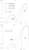 |
Fig. 5 Growth rates for the PFHI and the whistler instability (WI) as provided by Eq. (7) for Te,∥/Tp,∥ = 2, βe,∥ = 8, (βp,∥ = 4), Te,∥ ≃ 106 K, Tp,⊥/Tp,∥ = 0.25, and electrons with a small anisotropy Te,⊥/Te,∥ = 1.2 a), 1.5 b). (Wi = ωi/Ωp, K = kc/ωp,p). |
In the opposite case, when the electrons are hotter along the magnetic field direction, the EFHI is also expected to grow and compete with the PFHI (see Fig. 6). These instabilities interplay with each other and produce two maxima in the wave spectrum (see Fig. 6, panels b, c, and d)1. The PFHI grows at smaller wave numbers, and because the two peaks lie within a narrow wavenumber interval they can overlap if plasma conditions are favorable to only one of these instabilities. Three situations displayed in Fig. 6 are representative of the case where these growing modes produce two distinct maxima. We keep the electron anisotropy fixed (Te,⊥/Te,∥ = 0.5) and vary the proton anisotropy. At small deviations from isotropy (Tp,⊥/Tp,∥ = 0.8), the EFHI instability is usually much faster than the PFHI (panel c). Large anisotropies enhance the PFHI that becomes competitive (panel b), or even faster than the EFHI (panel d). In Kappa-distributed plasma, the tendency is the same, and the growth rates are diminished and restrained to small wave numbers because, in this case, the EFHI is suppressed much faster for decreasing values of κe,p. Towards the smallest values of κe,p, as illustrated, for instance, for the growth rates corresponding to κe = 2 and κp = 3 in panels b, c, and d, the EFHI is absent and the PFHI is only slightly inhibited.
These two instabilities have magnetic helicity of opposite sign (RH for the PFHI and LH for the EFHI) and this can help us to discriminate between the peaks, or to decide on their nature when they overlap. Changing of the sign of the oscillatory frequency (and the polarization) occurs exactly at the local minimum of the growth rate, when the PFHI mode shifts to the EFHI mode. This is clearly shown in Fig. 3, panels a and b. At small values of κe,p (e.g., κe = 2 and κp = 3), the frequency does not change sign because the PFHI is dominant and the EFHI is suppressed.
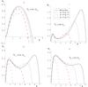 |
Fig. 6 The exact numerical solutions, the real frequency a), and the growth rate b), c), d) for the PFHI (small wave-numbers) and the EFHI (large wave-numbers) as provided by Eq. (7) for different indices κe,p, and typical solar wind plasma parameters Te,∥/Tp,∥ = 2, βe,∥ = 4, (βp,∥ = 2), Te,∥ ≃ 106 K and different anisotropies Te,⊥/Te,∥ = 0.5, Tp,⊥/Tp,∥ = 0.8 a), b), 0.4 c), 0.2 d). (Wr = ωr/Ωp, Wi = ωi/Ωp, K = kc/ωp,p). |
5. Conclusions
We have studied the influence of suprathermal populations on the dispersion properties of the PFHI. The excess of parallel kinetic energy (Tp,∥ > Tp,⊥) has been modeled with an anisotropic power law distribution of bi-Kappa-type.
In Sect. 2, we have derived the general dispersion relation of the RH transverse modes in terms of the modified plasma dispersion function for Kappa distributions. In the limits of both large or small arguments, this function admits approximative analytical forms, that allows us to identify the resonant and non-resonant contributions of the plasma particles. These limits have been explicitly described showing that in a Kappa-distributed plasma, the argument of the new plasma dispersion function becomes larger than unity for a large variety of plasma parameters, wave numbers, and frequencies. Thus, the approximation of the modified dispersion function given in Eq. (13) enables a simple analytical description of the unstable solutions.
Different plasma conditions favorable to an analytical description of the PFHI have been identified in Sect. 3. First, we have derived the threshold conditions, which become more stringent in Kappa-distributed plasmas: the PFHI requires a larger anisotropy and a larger plasma-β parameter to grow. To shape suprathermal distribution functions susceptible of producing the unstable fluctuations measured in solar wind, we have to determine values of the κe,p index satisfying the same condition in Eq. (15). Secondly, we have shown that even in the limit of small wave numbers the growth rates are sensitive to the form of the distribution function: growth rates decrease for low values of the κ index. The standard fluid-like model of the firehose instability is, therefore, recovered only in the Maxwellian limit of κ → ∞.
In Sect. 4, we have examined the exact numerical solutions of the PFHI. If the electrons are isotropic their effect is unimportant, but the influence of suprathermal populations depends on how large the proton anisotropy is. Thus, at large anisotropies the instability is enhanced with κp reaching a maximum for a Maxwellian (κp → ∞), but this tendency is restrained by decreasing the anisotropy, and for small anisotropies the growth rates decrease with κp.
The influence of suprathermal populations also depends on the electron anisotropy. If the electrons exhibit an excess of perpendicular temperature (Te,⊥ > Te,∥), the PFHI growth rates are enhanced by the suprathermal populations (at small values of κe,p) leading to a smooth transition into the whistler instability at high growth rates. In the opposite case, when the electrons are hotter along the magnetic field direction (Te,⊥ < Te,∥), both plasma components drive the firehose instability, the PFHI instability at small wave numbers and the EFHI at larger wave numbers. The growth rate dispersion curve exhibits two peaks of maximum, that can be distinct (Fig. 6), or can overlap when the conditions are favorable to only one of these instabilities. The advantage is that these two instabilities have magnetic helicity of opposite sign that can eventually discriminate the origin of the peaks. Within Kappa distributions, the tendency is the same, the growth rates being reduced and restrained to small wave numbers because the EFHI is suppressed much faster with decreasing κe,p.
The new properties of the PFHI presented here are expected to provide closer agreement with
measured data in the solar flares dominated by the suprathermal populations. If we consider
the magnetic fluctuations measured near 1 AU in the solar wind (Bale et al. 2009), the data distribution corresponding to the magnetic
fluctuation power is sharply peaked in a bandwith
kρp ≃ 0.56 ± 0.32, where
ρp = vp,th, ⊥ /Ωp
is the thermal proton gyroradius. Relating to our wave number scaled by the proton inertial
length 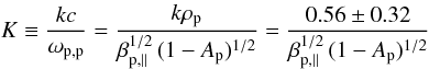 (30)and
assuming the solar wind plasma conditions adopted in Fig. 4, e.g., Ap = 3/4 and
βp,∥ = 4, the measured fluctuations
eventually generated by the PFHI must fall into a bandwith K = 0.24−0.88
that seems to be relevant for the branch of increasing (positive slope) growth rates
displayed in Figs. 4–6. We should, however, remember that these magnetic fluctuations are frequently
attributed to the oblique firehose instability that develops in the same conditions
(T∥ > T⊥),
and seems to be faster (Hellinger et al. 2006) than
the parallel firehose. Because a kinetic analytical treatment in two (or three) dimensions
is still a difficult task, here we have limited the study by considering only the parallel
propagation that must, however, retain the new features of this instability in
Kappa-distributed plasmas. Thus, the general trend of the instability thresholds moving to
larger values of β∥ (in Fig. 3) seems to agree with observations in the solar wind.
(30)and
assuming the solar wind plasma conditions adopted in Fig. 4, e.g., Ap = 3/4 and
βp,∥ = 4, the measured fluctuations
eventually generated by the PFHI must fall into a bandwith K = 0.24−0.88
that seems to be relevant for the branch of increasing (positive slope) growth rates
displayed in Figs. 4–6. We should, however, remember that these magnetic fluctuations are frequently
attributed to the oblique firehose instability that develops in the same conditions
(T∥ > T⊥),
and seems to be faster (Hellinger et al. 2006) than
the parallel firehose. Because a kinetic analytical treatment in two (or three) dimensions
is still a difficult task, here we have limited the study by considering only the parallel
propagation that must, however, retain the new features of this instability in
Kappa-distributed plasmas. Thus, the general trend of the instability thresholds moving to
larger values of β∥ (in Fig. 3) seems to agree with observations in the solar wind.
We thank the anonymous referee for pointing out this case of relevance from the perspective of observations.
Acknowledgments
We are grateful to the anonymous referee for his insightful comments and suggestions. The authors acknowledge financial support from the Research Foundation Flanders – FWO Belgium, the Katholieke Universiteit Leuven, and by the Deutsche Forschungsgemeinschaft (DFG), grant Schl 201/21-1. These results were obtained in the framework of the projects GOA/2009-009 (K.U. Leuven), G.0729.11 (FWO-Vlaanderen) and C 90205 (ESA Prodex 10). Financial support by the European Commission through the SOLAIRE Network (MTRN-CT-2006-035484) is gratefully acknowledged. The numerical results were obtained on the HPC cluster VIC of the K.U. Leuven.
References
- Bale, S., Kasper, J. C., Howes, G. G., et al. 2009, PRL, 103, 211101 [Google Scholar]
- Bougeret, J.-L., & Pick, M. 2007, in Handbook of Solar-Terrestrial Environment, Part 1, 133 [Google Scholar]
- Cairns, I. H., Robinson, P. A., & Zank, G. P. 2000, Publ. Astron. Soc. Aust., 17, 22 [Google Scholar]
- Chotoo, K., Schwadron, N., Mason, G., et al. 2000, J. Geophys. Res., 105, 23107 [NASA ADS] [CrossRef] [Google Scholar]
- Collier, M. R., Hamilton, D. C., Gloeckler, G., Bochsler, P., & Sheldon, R. B. 1996, Geophys. Res. Lett., 23, 1191 [NASA ADS] [CrossRef] [Google Scholar]
- Decker, D. B., Krimigis, S. M., Roelof, E. C., et al. 2005, Science, 309, 2020 [NASA ADS] [CrossRef] [PubMed] [Google Scholar]
- Dröge, W. 2003, ApJ, 389, 1027 [Google Scholar]
- Fisk, L. A., & Gloeckler, G. 2007, Space Sci. Rev., 130, 153 [Google Scholar]
- Dasso, S., Gratton, F. T., & Farrugia, C. J. 2003, JGR, 108, 1149 [CrossRef] [Google Scholar]
- Fried, B. D., & Conte, S. D. 1961, The Plasma Dispersion Function (New York: Academic Press) [Google Scholar]
- Gary, S. P. 1993, Theory of Space Plasma Microinstabilities (Cambridge: University Press) [Google Scholar]
- Gary, S. P., Montgomery, M. D., Feldman, W. C., & Forslund, D. W. 1976, JGR, 81, 1241 [Google Scholar]
- Gary, S. P., Li, H., O’Rourke, S., & Winske, D. 1998, JGR, 103, 14567 [NASA ADS] [CrossRef] [Google Scholar]
- Gloeckler, G., & Hamilton, D. C. 1987, Phys. Scripta T, 18, 73 [NASA ADS] [CrossRef] [Google Scholar]
- Hellinger, P., & Matsumoto, H. 2000, JGR, 105, 10519 [NASA ADS] [CrossRef] [Google Scholar]
- Hellinger, P., Travnicek, P., Kasper, J. C., & Lazarus, A. J. 2006, GRL, 33, L09101 [Google Scholar]
- Kasper, J. C., Lazarus, A. J., & Gary, S. P. 2002, GRL, 29, 1839 [Google Scholar]
- Lazar, M., & Poedts, S. 2009, A&A, 494, 311 [NASA ADS] [CrossRef] [EDP Sciences] [Google Scholar]
- Lazar, M., Schlickeiser, R., & Shukla, P. K. 2008a, Phys. Plasmas, 15, 042103 [NASA ADS] [CrossRef] [Google Scholar]
- Lazar, M., Schlickeiser, R., Poedts, S., & Tautz, R. C. 2008b, MNRAS, 390, 168 [NASA ADS] [CrossRef] [Google Scholar]
- Marsch, E. 2006, Liv. Rev. Sol. Phys., 3, http://www.livingreviews.org/lrsp-2006-1 [Google Scholar]
- Matteini, L., Landi, S., Hellinger, P., & Velli, M. 2006, JGR, 111, A10101 [NASA ADS] [CrossRef] [Google Scholar]
- Parker, E. N. 1958, Phys. Rev., 109, 1874 [NASA ADS] [CrossRef] [Google Scholar]
- Pierrard, V., & Lazar, M. 2010, Sol. Phys., 267, 153 [NASA ADS] [CrossRef] [Google Scholar]
- Pierrard, V., Lazar, M., & Schlickeiser, R. 2011, Sol. Phys. [Google Scholar]
- Pilipp, W., & Völk, H. J. 1971, J. Plasma Phys., 6, 1 [NASA ADS] [CrossRef] [Google Scholar]
- Quest, K. B., & Shapiro, V. D. 1996, JGR, 101, 24457 [NASA ADS] [CrossRef] [Google Scholar]
- Schlickeiser, R., Lazar, M., & Vukcevic, M. 2010, ApJ, 719, 1497 [NASA ADS] [CrossRef] [Google Scholar]
- Stverak, S., Travnicek, P., Maksimovic, M., et al. 2008, JGR, 113, A03103 [Google Scholar]
- Summers, D., & Thorne, R. M. 1991, Phys. Fluids B, 3, 1835 [NASA ADS] [CrossRef] [Google Scholar]
- Vasyliunas, V. M. 1968, JGR, 73, 2839 [Google Scholar]
- Xue, S., Thorne, R. M., & Summers, D. 1993, JGR, 98, 17475 [Google Scholar]
- Yoon, P. H. 1995, Phys. Scripta T, 60, 127 [NASA ADS] [CrossRef] [Google Scholar]
- Wang, B.-J., & Hau, L. -N. 2003, JGR, 108, 1463 [CrossRef] [Google Scholar]
All Figures
|
Fig. 1 Spectral domains R1–R4, where the approximations given in Eqs. (12) and (13) of the modified plasma dispersion function (8) can be used. For a dominance of suprathermal populations, indices κa → 1/2, and ακa → 0 increasing (meακeβe,∥/mp)−1/2 and (ακpβp,∥)−1/2 to very large values, and also enlarging the area where the arguments |ga| > 1 are large enough to apply the approximation in Eq. (13) for both species a = e,p, (Wr,i = ωr,i/Ωp, K = kc/ωp,p). |
| In the text | |
|
Fig. 2 Growth rates of the firehose instability as provided by Eq. (14) for κe = 2, κp = 3 (dotted line), κe,p = 4 (dashed line), κe,p → ∞ (solid line), and plasma parameters: Te,∥/Te,⊥ = Tp,∥/Tp,⊥ = 4, a) Te,∥/Tp,∥ = 3, βe,∥ = 18; and b) Te,∥/Tp,∥ = 2, βe,∥ = 8. For a given wave-number value K = 0.03, the growth rate variation with κe and κp is shown in panel c). (Wi = ωi/Ωp, K = kc/ωp,p). |
| In the text | |
|
Fig. 3 Threshold conditions for the EFHI (or the PFHI) as provided by Eq. (16) (or in Eq. (17)) for different
values κ. The instability occurs below the threshold lines for
|
| In the text | |
|
Fig. 4 The exact numerical solutions, the real frequency a) and the growth rate b), c), d) for the PFHI as provided by Eq. (7) for κp = 3 (dotted line), κp = 4 (dashed line), κp = 8 (long-dashed line), and κp → ∞ (solid line), and typical solar wind plasma parameters Te,∥/Tp,∥ = 2, βe,∥ = 8, (βp,∥ = 4), Te,⊥ = Te,∥ ≃ 106 K and different values of the proton anisotropy Tp,⊥/Tp,∥ = 0.25 a), b), 0.6 c), 0.8 d). Electrons are assumed to be isotropic and Maxwellian (κe → ∞). (Wr = ωr/Ωp, Wi = ωi/Ωp, K = kc/ωp,p). |
| In the text | |
|
Fig. 5 Growth rates for the PFHI and the whistler instability (WI) as provided by Eq. (7) for Te,∥/Tp,∥ = 2, βe,∥ = 8, (βp,∥ = 4), Te,∥ ≃ 106 K, Tp,⊥/Tp,∥ = 0.25, and electrons with a small anisotropy Te,⊥/Te,∥ = 1.2 a), 1.5 b). (Wi = ωi/Ωp, K = kc/ωp,p). |
| In the text | |
|
Fig. 6 The exact numerical solutions, the real frequency a), and the growth rate b), c), d) for the PFHI (small wave-numbers) and the EFHI (large wave-numbers) as provided by Eq. (7) for different indices κe,p, and typical solar wind plasma parameters Te,∥/Tp,∥ = 2, βe,∥ = 4, (βp,∥ = 2), Te,∥ ≃ 106 K and different anisotropies Te,⊥/Te,∥ = 0.5, Tp,⊥/Tp,∥ = 0.8 a), b), 0.4 c), 0.2 d). (Wr = ωr/Ωp, Wi = ωi/Ωp, K = kc/ωp,p). |
| In the text | |
Current usage metrics show cumulative count of Article Views (full-text article views including HTML views, PDF and ePub downloads, according to the available data) and Abstracts Views on Vision4Press platform.
Data correspond to usage on the plateform after 2015. The current usage metrics is available 48-96 hours after online publication and is updated daily on week days.
Initial download of the metrics may take a while.