| Issue |
A&A
Volume 533, September 2011
|
|
|---|---|---|
| Article Number | A10 | |
| Number of page(s) | 10 | |
| Section | Interstellar and circumstellar matter | |
| DOI | https://doi.org/10.1051/0004-6361/201117082 | |
| Published online | 12 August 2011 | |
VLBI imaging of a flare in the Crab nebula: more than just a spot
1
Max-Planck-Institut für Radioastronomie, Auf dem Hügel 69, 53121 Bonn, Germany
e-mail: This email address is being protected from spambots. You need JavaScript enabled to view it.
2
Institut für Experimentalphysik, University of Hamburg, Luruper Chaussee 149, 22761 Hamburg, Germany
3
Jodrell Bank Centre for Astrophysics, School of Physics and Astronomy, Alan Turing Building, University of Manchester, Manchester M13 9PL, UK
Received: 14 April 2011
Accepted: 1 July 2011
Abstract
We report on very long baseline interferometry (VLBI) observations of the radio emission from the inner region of the Crab nebula, made at 1.6 GHz and 5 GHz after a recent high-energy flare in this object. The 5 GHz data have provided only upper limits of 0.4 milli-Jansky (mJy) on the flux density of the pulsar and 0.4 mJy/beam on the brightness of the putative flaring region. The 1.6 GHz data have enabled imaging the inner regions of the nebula on scales of up to ≈ 40′′. The emission from the inner “wisps” is detected for the first time with VLBI observations. A likely radio counterpart (designated “C1”) of the putative flaring region observed with Chandra and HST is detected in the radio image, with an estimated flux density of 0.5 ± 0.3 mJy and a size of 0 2–06. Another compact feature (“C2”) is also detected in the VLBI image closer to the pulsar, with an estimated flux density of 0.4 ± 0.2 mJy and a size smaller than 02. Combined with the broad-band SED of the flare, the radio properties of C1 yield a lower limit of ≈ 0.5 mG for the magnetic field and a total minimum energy of 1.2 × 1041 erg vested in the flare (corresponding to using about 0.2% of the pulsar spin-down power). The 1.6 GHz observations provide upper limits for the brightness (0.2 mJy/beam) and total flux density (0.4 mJy) of the optical Knot 1 located at 06 from the pulsar. The absolute position of the Crab pulsar is determined, and an estimate of the pulsar proper motion (μα = −13.0 ± 0.2 mas/yr, μδ = + 2.9 ± 0.1 mas/yr) is obtained.
Key words: ISM: supernova remnants / radio continuum: stars / pulsars: general / pulsars: individual: Crab pulsar
Visiting Scientist, University of Hamburg/Deutsches Elektronen Synchrotron Forschungszentrum.
© ESO, 2011
1. Introduction
The inner region of the Crab nebula contains a complex and dynamic structure with a number of elliptical ripples (“wisps”) varying in flux on timescales of days and moving outward with speeds of up to 0.7 c (Tanvir et al. 1997; Hester et al. 2002) in the optical, while radio measurements with the VLA yield somewhat lower speeds of ≈ 0.3 c (Bietenholz et al. 2004). The origin of the wisps is not yet known, but they are generally thought to be associated with instabilities downstream of the shock in the wind from the pulsar that powers the nebula (Gallant & Arons 1994).
The wind derives its power from the pulsar spin-down injecting an energy of ~5 × 1038 erg/s into relativistic particles and magnetic field (Rees & Gunn 1974; Kennel & Coroniti 1984). The particles are thought to be mostly electrons and positrons, accelerated to relativistic energies, with possibly a lesser number of ions (Arons & Tavani 1994).
The exact mechanism by which the spin-down energy is released, transported, and dissipated remains poorly understood (cf., Chedia et al. 1997; Hester et al. 1998; Begelman 1999; Lyutikov 2003; Spitkovsky & Arons 2004; Komissarov & Lyubarsky 2004) – with shocks, plasma instabilities, pair acceleration, Poynting flux, and magnetic field all suggested to affect the evolution of the wind.
Fast variability possibly related to abrupt energy releases in the nebula was first reported in the radio on time scales of ~1 day, corresponding to an emitting region of  in size (Matveyenko 1975; Matveyenko & Kostenko 1979). On 22 September 2010, a gamma-ray flare was discovered for the first time from the direction of the Crab nebula with the AGILE pair-production telescope (Tavani et al. 2011), offering a rare opportunity to follow in detail the evolution of a flaring region in the nebula. The flare was confirmed with Fermi/LAT (Abdo et al. 2011) indicating a variability time-scale as short as 12 h (Balbo et al. 2011).
The flare was not detected in the keV regime with Swift/XRT (Evangelista et al. 2010) and INTEGRAL (Ferrigno et al. 2010b). The Fermi/LAT monitoring had further shown an abrupt decrease of the gamma-ray flux on 23 September, with the emission returning to its pre-flare level. Based on the short duration of the high-energy flare, it has been suggested (Komissarov & Lyutikov 2011) that the flaring material is located in the optical Knot 1 separated by  from the pulsar (Hester et al. 1995). However, subsequent high-resolution imaging with Chandra (on 28 September, Tennant et al.2010) revealed three stationary compact ( ≈ 1′′ in size) regions (labelled A, B, and C) of enhanced emission located on the X-ray bright ring. Similar structures are are also visible in an HST image of the Crab nebula taken on 02 October (Caraveo et al. 2010). These knots present themselves as a viable site for the flaring emission (Tavani et al. 2011), and their compactness may explain naturally the non-detections in observations with lower spatial resolution where the extended nebula emission dominates. The Chandra and HST observations of the knots indicate a strong, rapid, and efficient energy release in the flaring material and pose the question of the relation between the optical, X-ray, and gamma-ray emission. Given the position of the knots within the nebula (located not too far off the jet axis and slightly closer than the innermost wisp), it is not clear whether the flaring region is associated with the jet or with the equatorial outflow. Deciding on these issues relies on detailed imaging of the emitting region, which is best achieved in the radio regime.
We present here high-resolution wide-field radio images of the flaring knot and the central region of the nebula, obtained with very long baseline interferometry (VLBI) observations at a wavelength of 18 cm. These observations probe a wide range of angular scales, from ~10 milliarcsec to ~40 arcsec, detect the flaring region, and reveal, for the first time, the intricate morphological structure of the radio emission within about 20 parsecs of the pulsar. The observation and data reduction are described in Sect. 2. The resulting images are presented in Sect. 3, and discussed in the context of physics and evolution of the flare in the Crab nebula.
Antenna parameters.
2. Observations and data analysis
The flaring region was observed with VLBI on 5 November 2010 at 1.6 GHz (λobs = 18 cm) and on 23 November 2010 at 4.9 GHz (λobs = 6 cm). The total of eight EVN1 telescopes and three MERLIN2 telescopes participated in the observations, operating in e-VLBI3 mode. Basic parameters of the participating antennas and ranges of the respective baseline lengths, B, are given in Table 1.
The 1.6 GHz observations were made over 11 h at a central reference frequency of νobs = 1616.49 MHz. The 4.9 GHz observations were made over 8.2 h at a central reference frequency of νobs = 4948.74 MHz. The 6 cm and 18 cm observations have sampled ranges of visibility (uv) spacings, B/λ, of 2–36 × 106 λ (2–36 Mλ) and 0.01–49 Mλ, respectively (note that Hartebeesthoeck took part only in the 18 cm observation).
Target and calibrator sources.
For both observations, the field of view was centered on the position of the flaring region, Crab-A (Tavani et al. 2011), as measured from the HST data. The nearby bright (S1.6 GHz = 0.42 Jy) and compact radio source J0518+2054, separated by 4 0 from Crab-A, was used as a phase-reference calibrator. A calibrator/target cycle of 2/5 min was used, with about 30 s allocated for slewing. Two other calibrators, J0530+1331 and 3C 48, were observed as fringe finders. Positions and flux densities of the target and phase-reference calibrator are given in Table 2.
The EVN data were recorded at a rate of 1024 Megabit/s (Mbps), in dual-circular polarisation, which yielded and observing bandwidth of 128 MHz per polarisation. The total bandwidth was divided into 8 intermediate frequency (IF) bands, each covering 16 MHz and split in 32 spectral channels of 0.5 MHz in width. The MERLIN data were obtained at a 128 Mbps recoding rate, in dual-circular polarisation, yielding an observing bandwidth of 16 MHz per polarisation. The MERLIN data, corresponding to a single IF band of the EVN data, were recorded also using 32 spectral channels of 0.5 MHz in width, for each polarisation channel. The recording was made in a two-bit recording mode at all participating antennas. The resulting coverage of the Fourier domain (uv-coverage) provided by the visibility data on the target source is shown in Fig. 1, for the observations at 1.6 GHz.
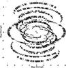 |
Fig. 1 Spatial frequency coverage (Fourier domain or uv-coverage) of the VLBI visibility data for the target source at 1.6 GHz. The coverage is plotted in Megawavelength (Mλ) units, referring to spatial frequencies of Bl,m/(λobs × 106), where Bl,m is the projected baseline length for a given pair of antennas (l,m). Baselines to Hartebeesthoeck, covering a range of 36–48.8 Mλ, are not shown. The smallest spatial frequency sampled is 10-2 Mλ, corresponding to ≈ 2 |
Correlation of the data was done at the EVN correlator facility of the Joint Institute for VLBI in Europe (JIVE). The output correlated data were produced with a 2 s averaging time. The combined choice of the integration time and the frequency channel width ensured that a field of view as large as 1 6 (at 1.6 GHz) and 05 (at 5 GHz) could be imaged using only the visibility data from the European baselines (B ≤ 10 Mλ) shown in Fig. 1, with the synthesised beam degraded by less than 10%. No pulsar gating was applied (this correlation mode is currently unavailable for e-VLBI observations).
The correlated data were processed using AIPS4 software. The data scans were first flagged using automatic flag tables produced during the correlation. The visibility amplitudes were calibrated, based on the system temperature measurements and station gain information. The data for the phase-reference calibrator were then fringe-fitted, and a bandpass calibration was applied. The phase-reference calibrator was imaged and found to have only a weak extended structure, ensuring that it was not contaminating the phase solutions. The phase solutions were then transferred to the target scans, and phase-calibrated data for the target source were imaged.
2.1. 5 GHz data
No positive detection of emission can be made from the 5 GHz data for the flaring region and for the pulsar itself, even in a heavily tapered image with a beam (FWHM) of  . The pulsar emission is reported to have a continuum flux density of 14.4 ± 3.2 mJy at 1.4 GHz and a very soft spectral index αpsr = −3.1 ± 0.2 (Lorimer et al. 1995). This corresponds to a flux density of ≈ 0.3 mJy at 5 GHz. We estimate an rms noise of σ6cm ≈ 0.16 mJy/beam, from the inverted 5 GHz visibility data. Thus the pulsar flux is expected to reach an ≈ 2σ level in the 5 GHz image. Based on these considerations, an upper limit of ~ 0.4 mJy can be provided for the flux density of the pulsar. The corresponding upper limit on the brightness of the knot A is then ~0.4 mJy/beam, for the above mentioned beam size.
The following discussion is therefore focused primarily on the results obtained from the VLBI data at 1.6 GHz.
2.2. Effects of the pulsar and extended nebula on imaging
The presence of the pulsar and an extremely large (420′′ × 290′′) and bright nebula results in an increase in the image noise level in the flaring region. For the antenna configuration used in the observation, sensitivity reductions by factors of 3.0 and 3.2 are expected for the EVN and MERLIN parts of the data, respectively. These estimates account for the 1.6 GHz flux density (~900 Jy) of the nebula and the primary beams response of the EVN and MERLIN antennas to the nebula. The resulting expected rms image noise in the combined data is ≈ 60 μJy/beam (in a full-resolution image made from naturally-weighted visibility data). The contribution of the pulsar to the image noise is not as significant. At the observing frequency of 1.6 GHz, the expected continuum flux of 8.6 mJy, and sidelobes from the pulsar resulting from deconvolution defects are expected to become relevant at a ~10 μJy/beam brightness level, which is lower than the estimated thermal noise.
2.3. Resolution and structural sensitivity
The visibility data at 18 cm sample a range of uv-spacings from 10-2 Mλ to 48.8 Mλ, with a large gap between 9 Mλ and 36 Mλ. The full-resolution, image made from the uniformly-weighted data, including the baselines to Hartebeesthoeck, has a synthesised beam with a full width at half maximum (FWHM) of 19.9 × 2.2 mas, while the European baselines yield a beam with a FWHM of 25.7 × 22.1 mas. The combination of angular scales sampled and flux density sensitivity of the data on the baselines to Hartebeesthoeck makes them useful only for imaging and astrometry of the pulsar itself.
The largest formally detectable scale in the data is about 20′′ ( ≈ 20% of the unaberrated field of view). However, this scale is sampled only by a single baseline, and a realistic limit on adequate structural sampling is  ( ≈ 1 Mλ), noting the gap in the uv-coverage shown in Fig. 1. This gap corresponds to angular scales of 02–2′′. It should be thus expected that smooth emission on scales larger than
  (and in the 02–2′′range in particular) could only be poorly recovered from the data (leading to “spotty” structures in images obtained using deconvolution, or requiring progressively higher signal-to-noise ratio on these scales in order to be successfully recovered by the maximum entropy method). The limited structural sensitivity of the VLBI data acts effectively as a low frequency uv-filter, reducing the contribution from large spatial scales where diffuse emission from the extended nebula dominates strongly. This leads to a better detectability of bright and compact regions which otherwise would have been swamped by the bright diffuse emission.
2.4. Imaging
Taking into account the issues of resolution and structural sensitivity outlined above, we have made three different images from the data: 1) a full-resolution image of a small region around the pulsar (Fig. 2); 2) a single-scale CLEAN image aiming at detecting the flaring region (Fig. 3); and 3) a multi-scale CLEAN image of extended emission within a region of about 40 in size (Fig. 4). The latter two images have been made using only the data from European baselines covering the uv-spacings of up to 10 Mλ (this has been done in order to improve the sensitivity to extended, low surface brightness emission). Properties of the images obtained are summarised in Table 3.
Properties of eVLBI images of the Crab nebula at 1.6 GHz.
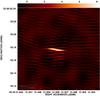 |
Fig. 2 Full resolution image of the Crab pulsar obtained from uniformly weighted data. The image has a peak flux density of 8.3 mJy/beam and an rms noise of 0.3 mJy/beam. The synthesised (restoring) beam is 19.9 × 2.2 mas, oriented at a PA = 83°. The extreme ellipticity of the restoring beam results from a very limited East-West uv-coverage on baselines ≥ 10 Mλ. |
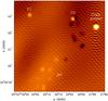 |
Fig. 3 Image of the pulsar and the flaring region. The image is obtained by applying a single-scale CLEAN deconvolution on the uv-tapered visibility data on the European baselines. The parameters of the image are given in Table 3. For the presentation purpose the image is convolved with a |

2.4.1. Pulsar
The full-resolution image of the Crab pulsar is made from the entire data, using the uniform weighting and restricting the field of view to  . A phase shift of
  in right ascension and
  is applied to the data in order to center the image on the location of the pulsar. The resulting high-resolution phase-referenced image of the pulsar is shown in Fig. 2.
Properties of the pulsar emission are estimated by fitting an elliptical Gaussian to the image brightness distribution. This yields an integrated flux density of 8.4 ± 0.5 mJy, which is close to the value estimated from the flux density measurements of Lorimer et al. (1995). Deconvolution of the fitted extent of the Gaussian indicates that the pulsar emission is not resolved, with the limits on its size obtained from the uncertainties of the fit σmaj = 0.40 mas (at a position angle of 81°) and σmin = 0.09 mas for the major and minor axis of the Gaussian, respectively. A similar estimate (σmaj = 0.40 mas, σmin = 0.04 mas) is obtained using from the SNR of detection of the pulsar emission.
2.4.2. Image of the flaring region
As described above, extended emission of the Crab nebula has been imaged with the data from the European baselines (B ≤ 10 Mλ), which has been done in order to improve the sensitivity to emission on scales ≳ 20 mas resolved out on the baselines to Hartebeesthoeck.
The visibility data are phase-shifted in right ascension by  , in order to fit better the field of interest within a rectangular grid. The grid extends by
  from the phase-center, thus covering almost the entire unaberrated field of view (allowing for about 5% reduction of the peak response due to bandwidth and time average smearing). As the flaring region is likely to be extended, the visibility data are weighted using the natural weighting and tapered using a Gaussian taper with σtaper = 2.2 Mλ. This yields a synthesised beam of 54 mas × 49 mas, which is about 2.5 times larger than the beam obtained without the taper.
The image of the flaring region shown in Fig. 3 is obtained by using single-scale CLEAN deconvolution and convolving the results with a larger beam  in order to enhance the contrast for the regions of weak, extended emission. The likely radio counterpart of the flaring component (denoted as C1) is clearly detected in this image, albeit at a somewhat smaller separation from the pulsar than the optical/X-ray emitting region Crab-A. The weak radio jet (located in the direction of the “sprite” identified in the HST images; cf., Hester et al.2002; Melatos et al.2005) and another, weaker but more compact component (C2) are also visible in the image. The possible nature of the two compact components and their relation to the flare will be discussed below.
The bright optical knot (Knot 1) seen in the HST images at a 06 distance from the pulsar (cf., Hester et al. 1995) is not detected in the 1.6 GHz image. An upper limit on its brightness is provided by the rms (0.2 mJy/beam) measured in the region where it is located. The non-detection of Knot 1 may imply both its weakness in the radio and large extension resulting in it being resolved out in the VLBI data. For the Knot 1 dimensions ( , Hester et al.1995), the upper limit on its total flux density at 1.6 GHz is ≈ 0.4 mJy.
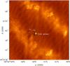 |
Fig. 4 Image of the central region of the Crab nebula obtained from naturally weighted data, uv-tapered data on baselines up to 10 Mλ. The image is obtained using a multi-scale CLEAN deconvolution and restored with a circular beam of |

2.5. Fidelity of detection of the compact features
The compact components C1 and C2 are strongly resolved, and they cannot be detected without tapering of the visibility data. This implies that their sizes should be a priori larger than ~40 mas and that both emitting regions most likely have a smooth extended structure that can be adequately imaged only with a dense sampling on short baselines (B ≤ 250 km). Because of the lack of such baselines in our data, the appearance and relative brightness of C1 and C2 depend on the choice of deconvolution and image restoration procedures. In the single-scale CLEAN image in Fig. 3, which is biased to higher spatial frequencies (hence smaller angular scales), the peak brightness is higher in the more compact feature C2. The multi-scale CLEAN image in Fig. 4 accounts better for lower spatial frequencies (larger angular scales), yielding a larger flux density for the more extended feature C1, with some of this emission possibly coming from the extended emission of the nearby “wisp”. Considering all these factors, and taking into account the likely angular extent of both components, we estimate that the application of single-scale CLEAN deconvolution yields detections at an SNR of 4.2 and 3.2, for C1 and C2 respectively. The respective SNR values are reduced to 3.8 and 2.5 in the multi-scale CLEAN image in which the cumulative spatial sensitivity is shifted to scales that are much larger than the angular extent of C1 and C2.
To test the fidelity of detection of such features in the EVN data, we supplement the visibility data with two sets of simulated Gaussian components representing C1 and C2 at different position angles and distances from the pulsar. The representations of C1 have a flux density of 0.5 mJy and a size of 02; the respective values for C2 are 0.4 mJy and 015. Random noise is added to the visibility data, to accommodate for the total signal increase due to the simulated features. As the sum flux density of the simulated components (1.8 mJy) represents only a small fraction of the total flux density in the image (140 mJy), the resulting noise factor is also relatively small and leads to an increase of the average visibility noise from 73.2 mJy to 74.1 mJy.
Locations of the first set (C1a, C2a) of the added components are obtained by rotation of the positions of C1 and C2 by − 122°. For the second set (C1b, C2b), a rotation by − 47° is combined with a factor of 4 stretch in distance from the pulsar. This ensures that the resulting locations of the simulated components span a range of pulsar separations, Δr, ranging from 16 to 164 and fall outside of the areas with detected emission. The modified data are then imaged using the same procedure as applied for obtaining the single-scale CLEAN image. All four simulated features are detected in the resulting image and the ratios, ζS, of their fluxes to the fluxes of the original components are close to unity (see Table 4), and only the most distant simulated feature shows a perceivable decrease in flux density, owing most likely to the smearing effects. These results support further the reliability of the detection of the compact features C1 and C2.
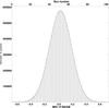 |
Fig. 5 Histogram of the residual flux distribution in the VLBI image, after applying the multi-scale CLEAN. The histogram is well approximated by the Gaussian noise (solid line) with an rms of 0.16 mJy/beam. |
Flux density ratios for simulated compact features.
2.5.1. Image of the central region of the nebula
Beyond the extent of the flaring region, the CLEAN algorithm finds positive flux as well, indicating likely detection of the two inner “wisps” visible in the optical and radio images obtained with HST and VLA (Bietenholz et al. 2004). As expected, this emission is not well recovered by CLEAN, resulting in a “spotty” appearance of the elliptically-shaped wisps. In order to improve the representation of large-scale structures in the image, we have applied multi-scale CLEAN (MS-CLEAN) algorithm.
Application of MS-CLEAN leads to moderate improvement of the image at large scales (Fig. 4), and it has also resulted in a moderate reduction of the rms noise in the image. The distribution of the residual flux in the image is shown in Fig. 5. The distribution is essentially Gaussian, implying an rms of 0.16 mJy/beam. At the same time, the application of multi-scale CLEAN has introduced a substantial power on scales  and thus reducing the contrast on smaller scales (which is visible in particularly in Fig. 4 at the location of the weaker feature C2).
The total CLEAN flux density in the image is 148 mJy, which reflects only a fraction of the total flux density in this area (as the VLBI data) do not sample spatial scales larger than 20′′and indeed have problems with recovering flux on spatial scales larger than about 02.
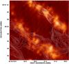 |
Fig. 6 The VLBI image of the Crab nebula (grey scale) overlaid with a VLA image (contours) of the same region obtained by Bietenholz et al. (2004). The VLBI image is obtained from the multi-scale CLEAN image by removing the contribution from the pulsar and restoring the resulting image with a 1 |
2.5.2. Fidelity of the large-scale structure
The large-scale structure detected in the image shown in Fig. 4 can be compared to the structure imaged with the VLA (Bietenholz et al. 2004). This comparison is presented in Fig. 6, which relates the VLA image to the multi-scale CLEAN image restored with a 14 beam (to match the VLA image resolution). The location and shape of the inner “wisps” agree well in the VLBI and VLA images. It should be noted of course that the two images are not contemporary, and thus the apparent agreement may be simply fortuitous. Nevertheless, this argues for the overall plausibility of the larger scale structure in the VLBI image.
One particularly remarkable difference between the structure seen in the VLA and VLBI images is observed in the south-western direction, where the VLBI image does not show any enhancement in flux, while a strong and extended emission region is visible in the VLA image. It is presently impossible to judge whether this disagreement is caused by the evolution of the radio emission or by deficiencies in the VLBI data and imaging. It should be noted however that this region is situated at more than 30′′( ≈ 600 beamwidths) away from the phase-center of the VLBI data, and the resulting reduction in peak response and beam deterioration may reduce detectability of weak and extended emission.
The imaging results summarised above indicate that the VLBI observations have not only been sensitive enough to detect the presence of a compact flaring emission in the Crab nebula, but they also enable obtaining a detectable response from the inner wisps of the nebula. However, the fidelity of localisation of this emission remains marginal, given the limited uv-coverage of the VLBI data. It is obvious that improved uv-coverage on shorter baselines is required in order to be able to image these structures, and a full-fledged combination of eMERLIN and EVN, both operating at 1 Gbit/s recording rates, would provide substantially better images of the central region in the Crab nebula.
The measured brightness of the wisps at 1.6 GHz and the rms estimate at 5 GHz can be reconciled with the “canonical” spectral index of α = −0.3 obtained in the radio regime for the total flux density of the nebula (Baars et al. 1977; Kovalenko et al. 1994) as well as for the resolved structures including the inner wisps (Bietenholz et al. 1997). The inner wisps detected in the VLBI image at 1.6 GHz have an average brightness of 0.3 mJy/beam. Adopting α = −0.3 yields an expected 5 GHz brightness of 0.2 mJy/beam, which compares well with the rms of 0.16 mJy/beam estimated from the 5 GHz data.
3. Results and discussion
The VLBI observations of the Crab nebula have yielded accurate positional and photometric information about the pulsar itself and the flaring region, as well as marginal morphological and photometric information about the inner wisps of the nebula.
3.1. Astrometry and proper motion of the pulsar
The position of the pulsar is measured relative to the position of the phase-reference calibrator, J0518+2054. The position of J0518+2054 has been determined with an accuracy of 0.12 mas, both in right ascension and declination (Petrov et al. 2008). The calibrator image obtained from the VLBI data shows no significant structure that could affect the calibrator phases and introduce additional positional errors. The total flux density recovered in the calibrator image is 290.1 ± 1.8 mJy, and the peak flux density is 271.0 ± 1.0 mJy/beam, further underlying the compactness of the structure. The calibrator image has a convolving beam of 18 × 12 mas and an rms noise of 0.8 mJy/beam (and the respective peak-to-noise SNR of 340), thus limiting the angular size of the calibrator to ≤ 1.1 mas and introducing an error of 0.06 mas to the positional measurements. For the calibrator, we obtain the following J2000 position (the errors listed are formal errors of the fit): 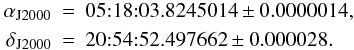 Analysis of the high-resolution image of the pulsar yields an apparent J2000 position (the errors are formal errors of the fit):
 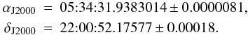 Taking into account the positional errors of the calibrator listed in Table 2, more conservative estimates of the errors of the pulsar position are given by Δα = 0.18 mas (0
 000012) and Δδ = 0.22 mas. These estimates do not include errors due tropospheric and ionospheric delays and errors from the calibrator-target phase transfer normally considered in measurements made with dedicated VLBI astrometry observations (cf., Guirado et al. 1995; Martí-Vidal et al. 2008). Based on the analysis of these factors (Guirado et al. 1995), we can expect that their contribution to the positional errors should be within ≈ 0.05 FWHM [mas] Δθ [deg] milliarcseconds, with Δθ giving the calibrator-target distance. For the FWHM of the full resolution image, one can therefore expect that the positional errors can reach Δα = 3.4 mas and Δδ = 0.45 mas (reflecting a much better north-south resolution of the image).
The position measurement made from the VLBI data can be combined with the Crab pulsar positions obtained from pulsar timing (Taylor et al. 1993; Han & Tian 1999), yielding the following estimate of the pulsar proper motion:  This estimate agrees well with recent estimates made from a long range of HST observations (Ng & Romani 2006; Kaplan et al. 2008).
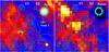 |
Fig. 7 Image of the radio emission (green contours; multi-scale CLEAN image, convolved with a 0 |


3.2. Flaring region
The flaring components C1 and C2 are both very weak, detected at SNR ≤ 4, which makes it difficult to provide robust estimates of their properties. Table 5 lists our best estimates of the positions, flux densities, and sizes of the two components, based on Gaussian fits to the single-scale and multi-scale image (with the latter providing a somewhat better account of the extent of the emitting regions). We use these positions to estimate brightness temperature of the emission in respective regions. The resulting values indicate brightness temperature in excess of ≈ 4000 K (it should be noted here that estimating such low values of brightness temperature is enabled by the presence of short baselines provided by the MERLIN antennas). The upper limit on the size of C1 corresponds to the maximum size of a 0.5 mJy feature that could be detected in the data.
Properties of compact flaring components.
An overlay of the radio image of the flaring region with an HST image from 2 October (Caraveo et al. 2010) and a Chandra image from 28 October (Ferrigno et al. 2010a) is shown in Fig. 7. The radio image is convolved with a 07 beam to further emphasise weak extended emission. This overlay shows that the radio emission traces well the inner wisp and “sprite” (region B), commonly identified in the optical/X-ray images. The radio component C1 is located close to a “knee-like” region (region A) detected in the optical and X-ray images and believed to be associated with the flare (Tavani et al. 2011). This morphology may also be reflected by the radio emission, but establishing this relation clearly requires better quality of radio imaging on arcsecond scales.
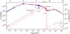 |
Fig. 8 The spectral energy distribution of the nebula and the flaring component C1. The data on the nebula have been compiled in Meyer et al. (2010). Details on the modelling of the synchrotron nebula are provided in that reference as well. In addition to the nebula, the SED of the feature C1 is shown together with a time-dependent model of the flare (solid red line), with spectra calculated at the epoch of the flare maximum (tf) and one day before (tf − 1d) and after (tf + 1d) the maximum. |
3.3. Origin of the radio knots
A significant offset of both C1 and C2 from the jet axis is evident. If these two features are associated with the jet (and are not part of the wisps produced in the equatorial outflow), it may be speculated that they are located on a “wall” formed by interaction of the rotating outflow with the ambient material in the nebula.
The offsets Δ r of C1 and C2 with respect to the jet axis, z, directed at a position angle ψjet ≈ 130° (estimated from the image in Fig. 3) can be represented by a power-law expansion Δ r ∝ zm, which yields m ≈ 0.7. A jet viewing angle of 60° (Cheng et al. 2000; Komissarov & Lyutikov 2011) is assumed in these calculations. The expansion derived is consistent with the one expected for the jet boundary in a magnetically confined flow (Fendt 1997; Fendt & Memola 2001) with a weakly evolving poloidal magnetic field component. One can assume that the jet boundary is defined by the outermost flux surface (cf., Fendt & Memola 2001) and that the collimation of the flow begins near the light cylinder, Rlc, with an initial radius of the flow of ≈ 10 Rlc. It would then require an electric current Ip ≈ 4 × 10¹⁴ A, a magnetic field B ≈ 4 × 10¹² G, and a magnetic flux Ψp ≈ 6 × 1024 G cm2 (all agreeing well with earlier estimates made for the Crab pulsar; cf., Hankins & Eilek2007; Hirotani2006) to explain the locations of the knots C1 and C2, assuming that these knots are located near the jet boundary. We note that the value of Ip is larger than the Goldreich-Julian current, which can be explained by pair cascades yielding particle densities well in excess of the Goldreich-Julian density (Arendt & Eilek 2002). With the jet expansion derived, the jet should have local half-opening angles of φC1 = 27° and φC2 = 37° at the locations of the radio knots. For the HST Knot 1, the respective half-opening angle is φHST 1 = 56°, which is close to the value of 60° expected for this region (Komissarov & Lyutikov 2011). These arguments lend further support to the suggestion that the radio knots are connected to the outflow. However, providing a firm conclusion on this matter would certainly require a closer followup of another prominent flare in the Crab nebula.
3.4. Connection to the high-energy flare
Based on the observational results summarised above, the faint and compact radio features C1 and C2 could in principle be related to the gamma-ray flare, even if they are not co-spatial with the active regions observed in the optical and X-ray bands. In the following, we consider a scenario in which the brighter feature C1 is related to the gamma-ray flare and discuss the consequences.
The spectral energy distribution (SED) of C1 is shown in Fig. 8 together with the nebula emission (see Meyer et al. 2010, for details of the data). This SED combines the flux density measured at 1.6 GHz, the upper limit obtained at 5 GHz, and the X-ray flux of the knot A treated here as a (soft) upper limit on the X-ray emission from the immediate vicinity of C1. Assuming that the underlying particle distribution present in the region C1 has the same spectral slope (dn/dγ = n0γ-1.60) as the electrons responsible for radio emission in the nebula, the resulting spectrum matches quite well both the radio as well as the gamma-ray emission across 14 orders of magnitude in energy.
The observed variability time-scale of about 24 h (Balbo et al. 2011) constrains the size of the emitting region to be smaller than  . This is consistent with the observed extension of C1. Assuming that the gyro-radius rg < ctvar and that gamma-rays are produced via synchrotron emission, a lower limit on the B-field is set by B ≥ 0.5 mG (E/100 MeV)1/3(tvar/100 ks) − 2/3. A conservative upper limit on the magnetic field of ≈ 100 mG follows from the argument that the total energy in the magnetic field should not exceed the spin down power of the pulsar integrated over the duration of the flare. The equipartition magnetic field (assuming minimum total energy) is Beq = 3 mG (tvar/100 ks) − 6/7(E/100 MeV)1/7. The corresponding total minimum energy (wtot = we + wB = 1.2 × 1041 erg). The injection power required to generate the burst is ẇ ≈ wtot/tvar = 1.2 × 1036 erg/s = 0.2% of the available spin-down power. Even though this is a comfortable margin, deviations from the minimum energy requirement are limited to roughly one order of magnitude.
Given the limited knowledge about the dynamics of the feature C1, it is difficult to estimate directly any effects related to relativistic beaming. A kinematic estimate of the Doppler factor  by adopting a jet viewing angle ϑ = 30° favoured in several recent works (e.g., Ng & Romani 2004; Komissarov & Lyubarsky 2004; Komissarov & Lyutikov 2011) and assuming that the jet material moves at a speed similar to the range of speeds observed in the wisps. This yields Doppler factors in a 1.4–1.8 range. An upper limit on the
  can also be derived based upon the non-observation of an accompanying flare at very high energy gamma-rays. The contemporaneous observations using the VERITAS and MAGIC (Mariotti 2010; Ong 2010) air Cherenkov telescopes rule out any substantial deviations of the flux in the energy regime between 100 GeV and TeV. Taking the relative flux errors of roughly 10% as an upper limit on any additional flaring component, we can estimate an upper limit on
  . The actual upper limit depends critically on the geometry. For the sake being conservative, we assume a synchrotron self-Compton type scenario neglecting additional photon fields.
These considerations (spectrum and size) are consistent with the hypothesis that the region C1 detected in the radio image is connected with the high-energy flare in the Crab nebula. The unusually long duration of higher flux state during this event may receive further support from the detection of C2, which could be a second plasma condensation ejected from the pulsar after the main flare in September 2010 and leading to emission enhancement in the high-energy regime.
The observed positional offset between the features C1 and A and the lack of obvious optical/X-ray counterparts for the feature C2 raise general questions of the relation between the emission detected in all three bands and the nature of the flaring activity in the Crab nebula. In the absence of better quality data, these questions remain open. As a matter of speculation, one can suggest that the flaring activity may be occurring in a relatively thin layer close to the jet boundary, thus highlighting the jet edges where the path length through the emitting material is larger (indeed, the locations of the features A and C can also be reconciled with the same jet expansion as derived above for C1 and C2). Such an activity may originate, for instance, from the magnetic reconnection or interaction of the jet with the ambient medium. However, in the absence of more detailed observational data, it is clearly not feasible to provide a reliable judgement on this matter.
In this respect, we also would like to emphasise that further improvement of the quality of radio imaging on arcsecond scales (which should be expected after the e-MERLIN becomes fully operational) would provide much better reliability for imaging of such extended and complicated objects as the central regions of the Crab nebula. Therefore, engaging in a detailed monitoring program of the Crab nebula with the EVN and e-MERLIN combined would be a highly desirable option for a followup of any future strong flaring event in this object.
European VLBI Network, www.evlbi.org
Multi Element Radio Linked Interferometer Network, www.merlin.ac.uk
Electronic-VLBI, a mode of VLBI operations, with direct links between participating telescopes and the correlator maintained via optical fibre connections; http://services.jive.nl/evlbi/
Astronomical Image Processing Software, National Radio Astronomy Observatory, USA.
Acknowledgments
A.P.L. acknowledges support from the Collaborative Research Center SFB 676 (Sonderforschungsbereich) “Particle, Strings, and the Early Universe” funded by the German Research Society (Deutsche Forschungsgemeinschaft). We are grateful to Michael Bietenholz for providing a VLA image of the Crab nebula. We thank the anonymous referee for constructive and helpful comments on the manuscript.
References
- Abdo, A. A., Ackermann, M., Ajello, M., et al. 2011, Science, 331, 739 [NASA ADS] [CrossRef] [PubMed] [Google Scholar]
- Arendt, Jr., P. N., & Eilek, J. A. 2002, ApJ, 581, 451 [NASA ADS] [CrossRef] [Google Scholar]
- Arons, J., & Tavani, M. 1994, ApJS, 90, 797 [NASA ADS] [CrossRef] [Google Scholar]
- Baars, J. W. M., Genzel, R., Pauliny-Toth, I. I. K., & Witzel, A. 1977, A&A, 61, 99 [NASA ADS] [Google Scholar]
- Balbo, M., Walter, R., Ferrigno, C., & Bordas, P. 2011, A&A, 527, L4 [NASA ADS] [CrossRef] [EDP Sciences] [Google Scholar]
- Begelman, M. C. 1999, ApJ, 512, 755 [NASA ADS] [CrossRef] [Google Scholar]
- Bietenholz, M. F., Kassim, N., Frail, D. A., et al. 1997, ApJ, 490, 291 [NASA ADS] [CrossRef] [Google Scholar]
- Bietenholz, M. F., Hester, J. J., Frail, D. A., & Bartel, N. 2004, ApJ, 615, 794 [NASA ADS] [CrossRef] [Google Scholar]
- Caraveo, P., de Luca, A., Mignani, R., et al. 2010, The Astronomer’s Telegram, 2903, 1 [NASA ADS] [Google Scholar]
- Chedia, O., Lominadze, J., Machabeli, G., McHedlishvili, G., & Shapakidze, D. 1997, ApJ, 479, 313 [NASA ADS] [CrossRef] [Google Scholar]
- Cheng, K. S., Ruderman, M., & Zhang, L. 2000, ApJ, 537, 964 [NASA ADS] [CrossRef] [Google Scholar]
- Evangelista, Y., Campana, R., Capalbi, M., et al. 2010, The Astronomer’s Telegram, 2866, 1 [NASA ADS] [Google Scholar]
- Fendt, C. 1997, A&A, 323, 999 [NASA ADS] [Google Scholar]
- Fendt, C., & Memola, E. 2001, A&A, 365, 631 [NASA ADS] [CrossRef] [EDP Sciences] [Google Scholar]
- Ferrigno, C., Tennant, A., Horns, D., et al. 2010a, The Astronomer’s Telegram, 2994, 1 [Google Scholar]
- Ferrigno, C., Walter, R., Bozzo, E., & Bordas, P. 2010b, The Astronomer’s Telegram, 2856, 1 [NASA ADS] [Google Scholar]
- Gallant, Y. A., & Arons, J. 1994, ApJ, 435, 230 [NASA ADS] [CrossRef] [Google Scholar]
- Guirado, J. C., Marcaide, J. M., Elosegui, P., et al. 1995, A&A, 293, 613 [NASA ADS] [Google Scholar]
- Han, J. L., & Tian, W. W. 1999, A&AS, 136, 571 [NASA ADS] [CrossRef] [EDP Sciences] [Google Scholar]
- Hankins, T. H., & Eilek, J. A. 2007, ApJ, 670, 693 [NASA ADS] [CrossRef] [Google Scholar]
- Hester, J. J., Scowen, P. A., Sankrit, R., et al. 1995, ApJ, 448, 240 [NASA ADS] [CrossRef] [Google Scholar]
- Hester, J. J., Stapelfeldt, K. R., & Scowen, P. A. 1998, AJ, 116, 372 [NASA ADS] [CrossRef] [Google Scholar]
- Hester, J. J., Mori, K., Burrows, D., et al. 2002, ApJ, 577, L49 [NASA ADS] [CrossRef] [Google Scholar]
- Hirotani, K. 2006, ApJ, 652, 1475 [NASA ADS] [CrossRef] [Google Scholar]
- Kaplan, D. L., Chatterjee, S., Gaensler, B. M., & Anderson, J. 2008, ApJ, 677, 1201 [NASA ADS] [CrossRef] [Google Scholar]
- Kennel, C. F., & Coroniti, F. V. 1984, ApJ, 283, 710 [NASA ADS] [CrossRef] [Google Scholar]
- Komissarov, S. S., & Lyubarsky, Y. E. 2004, MNRAS, 349, 779 [NASA ADS] [CrossRef] [Google Scholar]
- Komissarov, S. S., & Lyutikov, M. 2011, MNRAS, 414, 2017 [NASA ADS] [CrossRef] [Google Scholar]
- Kovalenko, A. V., Pynzar’, A. V., & Udal’Tsov, V. A. 1994, Astron. Rep., 38, 78 [NASA ADS] [Google Scholar]
- Lorimer, D. R., Yates, J. A., Lyne, A. G., & Gould, D. M. 1995, MNRAS, 273, 411 [NASA ADS] [CrossRef] [Google Scholar]
- Lyutikov, M. 2003, MNRAS, 339, 623 [NASA ADS] [CrossRef] [Google Scholar]
- Mariotti, M. 2010, The Astronomer’s Telegram, 2967, 1 [Google Scholar]
- Martí-Vidal, I., Marcaide, J. M., Guirado, J. C., Pérez-Torres, M. A., & Ros, E. 2008, A&A, 478, 267 [NASA ADS] [CrossRef] [EDP Sciences] [Google Scholar]
- Matveyenko, L. I. 1975, Sov. Astr. Lett., 7, 13 [Google Scholar]
- Matveyenko, L. I., & Kostenko, V. I. 1979, Aust. J. Phys., 32, 105 [NASA ADS] [Google Scholar]
- Melatos, A., Scheltus, D., Whiting, M. T., et al. 2005, ApJ, 633, 931 [NASA ADS] [CrossRef] [Google Scholar]
- Meyer, M., Horns, D., & Zechlin, H. 2010, A&A, 523, A2 [NASA ADS] [CrossRef] [EDP Sciences] [Google Scholar]
- Ng, C., & Romani, R. W. 2004, ApJ, 601, 479 [NASA ADS] [CrossRef] [Google Scholar]
- Ng, C., & Romani, R. W. 2006, ApJ, 644, 445 [NASA ADS] [CrossRef] [Google Scholar]
- Ong, R. A. 2010, The Astronomer’s Telegram, 2968, 1 [Google Scholar]
- Petrov, L., Kovalev, Y. Y., Fomalont, E. B., & Gordon, D. 2008, AJ, 136, 580 [NASA ADS] [CrossRef] [Google Scholar]
- Rees, M. J., & Gunn, J. E. 1974, MNRAS, 167, 1 [NASA ADS] [CrossRef] [Google Scholar]
- Spitkovsky, A., & Arons, J. 2004, ApJ, 603, 669 [NASA ADS] [CrossRef] [Google Scholar]
- Tanvir, N. R., Thomson, R. C., & Tsikarishvili, E. G. 1997, New A, 1, 311 [Google Scholar]
- Tavani, M., Bulgarelli, A., Vittorini, V., et al. 2011, Science, 331, 736 [NASA ADS] [CrossRef] [PubMed] [Google Scholar]
- Taylor, J. H., Manchester, R. N., & Lyne, A. G. 1993, ApJS, 88, 529 [NASA ADS] [CrossRef] [Google Scholar]
- Tennant, A., Caraveo, P., Costa, E., et al. 2010, The Astronomer’s Telegram, 2882, 1 [Google Scholar]
All Tables
All Figures
|
Fig. 1 Spatial frequency coverage (Fourier domain or uv-coverage) of the VLBI visibility data for the target source at 1.6 GHz. The coverage is plotted in Megawavelength (Mλ) units, referring to spatial frequencies of Bl,m/(λobs × 106), where Bl,m is the projected baseline length for a given pair of antennas (l,m). Baselines to Hartebeesthoeck, covering a range of 36–48.8 Mλ, are not shown. The smallest spatial frequency sampled is 10-2 Mλ, corresponding to ≈ 2 |
| In the text | |
|
Fig. 2 Full resolution image of the Crab pulsar obtained from uniformly weighted data. The image has a peak flux density of 8.3 mJy/beam and an rms noise of 0.3 mJy/beam. The synthesised (restoring) beam is 19.9 × 2.2 mas, oriented at a PA = 83°. The extreme ellipticity of the restoring beam results from a very limited East-West uv-coverage on baselines ≥ 10 Mλ. |
| In the text | |
|
Fig. 3 Image of the pulsar and the flaring region. The image is obtained by applying a single-scale CLEAN deconvolution on the uv-tapered visibility data on the European baselines. The parameters of the image are given in Table 3. For the presentation purpose the image is convolved with a |
| In the text | |
|
Fig. 4 Image of the central region of the Crab nebula obtained from naturally weighted data, uv-tapered data on baselines up to 10 Mλ. The image is obtained using a multi-scale CLEAN deconvolution and restored with a circular beam of |
| In the text | |
|
Fig. 5 Histogram of the residual flux distribution in the VLBI image, after applying the multi-scale CLEAN. The histogram is well approximated by the Gaussian noise (solid line) with an rms of 0.16 mJy/beam. |
| In the text | |
|
Fig. 6 The VLBI image of the Crab nebula (grey scale) overlaid with a VLA image (contours) of the same region obtained by Bietenholz et al. (2004). The VLBI image is obtained from the multi-scale CLEAN image by removing the contribution from the pulsar and restoring the resulting image with a 1 |
| In the text | |
|
Fig. 7 Image of the radio emission (green contours; multi-scale CLEAN image, convolved with a 0 |
| In the text | |
|
Fig. 8 The spectral energy distribution of the nebula and the flaring component C1. The data on the nebula have been compiled in Meyer et al. (2010). Details on the modelling of the synchrotron nebula are provided in that reference as well. In addition to the nebula, the SED of the feature C1 is shown together with a time-dependent model of the flare (solid red line), with spectra calculated at the epoch of the flare maximum (tf) and one day before (tf − 1d) and after (tf + 1d) the maximum. |
| In the text | |
Current usage metrics show cumulative count of Article Views (full-text article views including HTML views, PDF and ePub downloads, according to the available data) and Abstracts Views on Vision4Press platform.
Data correspond to usage on the plateform after 2015. The current usage metrics is available 48-96 hours after online publication and is updated daily on week days.
Initial download of the metrics may take a while.