| Issue |
A&A
Volume 533, September 2011
|
|
|---|---|---|
| Article Number | A127 | |
| Number of page(s) | 6 | |
| Section | Numerical methods and codes | |
| DOI | https://doi.org/10.1051/0004-6361/201117051 | |
| Published online | 14 September 2011 | |
A 3D radiative transfer framework
VIII. OpenCL implementation
1
Hamburger Sternwarte, Gojenbergsweg 112,
21029
Hamburg,
Germany
e-mail: yeti@hs.uni-hamburg.de
2
Homer L. Dodge Dept. of Physics and Astronomy, University of
Oklahoma, 440 W. Brooks, Rm
100, Norman,
OK
73019,
USA
e-mail: baron@ou.edu
3
Computational Research Division, Lawrence Berkeley National
Laboratory, MS 50F-1650, 1
Cyclotron Rd, Berkeley, CA
94720-8139,
USA
Received: 8 April 2011
Accepted: 18 July 2011
Aims. We discuss an implementation of our 3D radiative transfer (3DRT) framework with the OpenCL paradigm for general GPU computing.
Methods. We implemented the kernel for solving the 3DRT problem in Cartesian coordinates with periodic boundary conditions in the horizontal (x,y) plane, including the construction of the nearest neighbor Λ∗ and the operator splitting step.
Results. We present the results of both a small and a large test case and compare the timing of the 3DRT calculations for serial CPUs and various GPUs.
Conclusions. The latest available GPUs can lead to significant speedups for both small and large grids compared to serial (single core) computations.
Key words: radiative transfer / methods: numerical
© ESO, 2011
1. Introduction
In a series of papers (Hauschildt & Baron 2006; Baron & Hauschildt 2007; Hauschildt & Baron 2008, 2009; Baron et al. 2009; Hauschildt & Baron 2010; Seelmann et al. 2010, hereafter: Papers I–VII), we have described a framework for solving the radiative transfer equation in 3D systems (3DRT), including a detailed treatment of scattering in continua and lines with a nonlocal operator splitting method and its use in the general model atmosphere package PHOENIX.
The 3DRT framework discussed in the previous papers of this series requires very substantial amounts of computing time owing to the complexity of the radiative transfer problem in strongly scattering environments. The standard method of speeding up these calculations is to implement parallel algorithms for distributed memory machines using the MPI library (Hauschildt & Baron 2006; Baron & Hauschildt 2007). The development of relatively inexpensive graphic processing units (GPUs) with large numbers of cores and the development of relatively easily used programming models, OpenCL and CUDA has made the use of GPUs attractive for accelerating scientific simulations. GPUs are built to handle numerous lightweight parallel threads simultaneously and to offer theoretical peak performance far beyond that of current CPUs. However, using them efficiently requires different programming methods and algorithms than those employed on standard CPUs. We describe our first results of implementing our 3DRT framework for a single geometry within the OpenCL (Munshi 2009) paradigm for generalized GPU and CPU computing.
2. Method
In the following discussion we use the notation in Papers I−VII. The basic framework and the methods used for the formal solution and the solution of the scattering problem via nonlocal operator splitting are discussed in detail in these papers and are not repeated here. Our implementation of the 3DRT framework considers the most time-consuming parts of the process – the formal solution and the solution of the operator splitting equations – to obtain the updated values of the mean intensities, whereas less time-consuming parts of the code (set-up, Ng acceleration, etc.) are left to Fortran95 or C implementations. The OpenCL implementation of the 3DRT framework minimizes data transfer between the host computer (CPU) and the GPU and keeps most of the data locally on the GPU memory. Only the relevant input data (e.g., opacities) and the results, e.g., the mean intensities J for all voxels, need to be transferred to and from the GPU device.
2.1. General purpose computing on graphic processors
Using a GPU for numerical calculations requires special programming environments. While GPU manufacturers have provided programming environments for vendor-special hardware, e.g., CUDA (NVIDIA 2007) for NVIDIA produced GPUs and ATI Stream SDK (AMD 2009) (which has now been replaced by AMD APP (AMD 2011) which uses OpenCL) for AMD/ATI produced GPUs. The differences between these environments make programs specific to systems from their respective vendors. Our applications need to be extremely portable, so having to code for multiple vendor-specific environments is not acceptable. Fortunately, the open standard OpenCL (Munshi 2009) was designed to efficiently use not only GPUs but also modern multicore CPUs and other accelerators using a thread-centered programming model. With OpenCL it is possible to run the same code on many different CPU and GPU architectures. There is a relatively minor cost with some loss of performance when using OpenCL rather than CUDA specific programming models (Komatsu et al. 2011). This is insignificant for our application where portability is far more important than the fraction of the theoretical peak performance attained for a specific piece of hardware. At the present time, OpenCL is available for all types of GPUs and CPUs, including accelerators such as the Cell Broadband Engine (CBE), whereas CUDA is only available for NIVIA GPUs. This is a major concern for us with the technology progressing rapidly and new hardware released frequently. Using a defined standard is, therefore, already important for building a reliable code base that can be used easily in the future. Maintaining several different codes for the same tasks in different programming languages is, on the other hand, costly in terms of human time and is also error prone. The disadvantage of this use of general standards is a small loss of performance. We consider this a low price for the portability because hardware features and performance increase dramatically with new hardware. Therefore, we implemented our 3DRT framework in OpenCL for portability reasons.
The design of GPUs differs considerably from the design of CPUs, focusing much more on simultaneous execution of many threads to hide memory access latencies. In contrast to CPUs, branching is costly on GPUs and should therefore be limited as much as possible. It is in many cases faster to compute both branches of a decision and then select the correct one afterwards rather than using conditional execution. This is not an uncommon strategy and it was used, for example, on the original CRAY vector machines in the 1980s. In addition, GPUs provide better performance for regular memory-access patterns. The preferred programming model for these GPU systems is a single-program, multiple-data (SPMD) type scheme that is directly supported by OpenCL. Branching within a program is allowed in this model, but often drastically reduces performance and thus should be avoided.
2.2. Implementation of the formal solution and Λ∗ computation
As a first step, we have implemented the “simplest” formal solution kernel in OpenCL. This is the kernel for Cartesian coordinates with periodic boundary conditions in the (horizontal) x − y plane discussed in Hauschildt & Baron (2008). An OpenCL implementation of the formal solution is in principle straightforward: For any given direction of photon propagation, all characteristics can be tracked simultaneously through the voxel grid, which corresponds to a 2D kernel in the OpenCL paradigm. The characteristics are started on the inner or outer x − y planes. The only substantial hurdle in the problem is that OpenCL (version 1.0 or 1.1) does not have facilities for atomic updates of floating point variables. This is, however, necessary for the numerically correct operation of a straightforward implementation of the formal solution for the calculation of the mean intensities and the Λ∗ operator. Therefore, we have implemented a 2-pass kernel, where in the first pass the intensities (etc.) are computed and stored along the characteristics that can be implemented with atomic operations on integer variables when the results are stored per voxel rather than per characteristic. In a second pass, these data are collected on a per voxel (3D) OpenCL kernel. With this method, the results are identical (to the precision used in the OpenCL implementation) to the Fortran95 implementation. However, the 2-pass method requires additional memory on the GPU to store the intermediate results and the first pass generates complex memory access patterns that are likely to limit performance on GPU based systems.
2.3. Implementation of the operator splitting step
The second very time-consuming part of the 3DRT framework is the solution of the operator splitting equations for computing the new values of the mean intensities J for all voxels. The Fortran95 code solves these equations by Jordan or Gauss-Seidel iterations. In OpenCL, it is much simpler to implement the Jordan method since it requires less synchronization between threads than does the Gauss-Seidel method. The OpenCL implementation uses a 3D kernel (all voxels simultaneously) and locally buffers the Λ∗ during the iterations, which dramatically speeds up the calculations.
3. Results
3.1. Test case setup
The test cases we have investigated follow the continuum tests used in Hauschildt & Baron (2008). In detail, we used the configuration for the testing where periodic boundary conditions (PBCs) are realized in a plane parallel slab. We used PBCs on the x and y axes and zmax is at the outside boundary, zmin the inside boundary. The slab has a finite optical depth in the z axis. The gray continuum opacity is parameterized by a power law in the continuum optical depth τstd in the z axis. The basic model parameters are
-
1.
the total thickness of the slab,zmax − zmin = 107 cm;
-
2.
the minimum optical depth in the continuum,
 and the maximum optical depth in the continuum,
  ;
; -
3.
an isothermal slab, T = 104 K;
-
4.
boundary conditions with outer boundary condition
 and inner boundary condition LTE diffusion for all wavelengths;
 -
5.
parameterized coherent & isotropic continuum scattering given by
 with 0 ≤ ϵc ≤ 1. κc and σc are the continuum absorption and scattering coefficients.
For the tests presented here, we used ϵc = 10-2 in order to allow single-precision runs, and double-precision is required for smaller epsilons for the solution of the operator splitting equations.
We have verified that the OpenCL calculations give the same result as the Fortran95 CPU calculations for the formal solution (intensities), the mean intensities, and the Λ∗. Likewise the solution of the 3D radiative transfer problem is the same for both OpenCL and Fortran95. For OpenCL single-precision calculations, the relative accuracy is about 10-5, which is acceptable for most calculations.
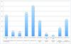 |
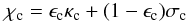
Fig. 1 Timing of the small 3D radiative transfer test calculation on CPUs (leftmost column), various GPUs with OpenCL, and multicore CPUs using OpenCL. The times are given in seconds of wallclock time. |
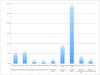 |
Fig. 2 Speed-ups of the small 3D radiative transfer test calculation for the OpenCL implementation relative to the serial CPU run. |
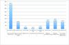 |
Fig. 3 Timing of the large 3D radiative transfer test calculation on CPUs (leftmost column), various GPUs with OpenCL, and multicore CPUs using OpenCL, MPI and OpenMP. The MPI calculation was run on 4 cores (1 CPU), the OpenMP run used 16 threads (8 cores, incl. hyperthreading) to be comparable to the OpenCL CPU run. The times are given in seconds of wallclock time. |
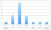 |
Fig. 4 Speed-ups of the large 3D radiative transfer test calculation for the OpenCL, OpenMP, and MPI implementations relative to the serial CPU run. The MPI calculation was run on 4 cores (1 CPU), and the OpenMP run used 16 threads (8 cores, incl. hyperthreading) to be comparable to the OpenCL CPU run. |
3.2. Timing results
In Figs. 1–4 we show the timing and speed-up results for small and large test cases. The difference between the tests is simply the size of the voxel grid. In the small case, we use 653 = 274 625 voxels, whereas the large test case uses a grid with 1292 ∗ 193 = 3 211 713 voxels. The small test cases uses 95.3 MB OpenCL memory in single-precision (165.5 MB double-precision) and thus fits easily in GPU devices with little memory, whereas the large test case uses 1.1 GB OpenCL memory in single-precision (1.9 GB in double-precision) and can thus only be used on high-end GPU devices. The tests were run on a variety of systems, from laptops with low-end GPUs to Xeon-based systems with dedicated GPU based numerical accelerator boards. For the comparisons in the figures, we have selected the fastest CPU run as the serial baseline for all comparisons. The systems used in the tests are:
-
1.
serial CPU: Mac Pro with OSX 10.6.4 and Intel Fortran 11.1, theCPU is a Xeon E5520 with 2.27 GHzclock-speed;
-
2.
MPI: 4 processes on Mac Pro with OSX 10.6.4 and Intel Fortran 11.1, the CPU is a Xeon E5520 (4 cores) with 2.27 GHz clock-speed;
-
3.
AMD/ATI Radeon HD 4870 GPU with 512 MB RAM on a Mac Pro with OSX 10.6.4 OpenCL;
-
4.
NVIDIA GeForce 8600M GT GPU with 512 MB RAM on a MacBook Pro laptop with OSX 10.6.4 OpenCL;
-
5.
NVIDIA GeForce GT 120 GPU with 512 MB RAM on a Mac Pro with OSX 10.6.4 OpenCL;
-
6.
NVIDIA Quadro FX 4800 GPU with 1536 MB RAM on a Mac Pro with OSX 10.6.4 OpenCL;
-
7.
NVIDIA GeForce 8800GT GPU with 512 MB RAM on a Linux PC with NVIDIA OpenCL (OpenCL 1.1, CUDA 3.2.1);
-
8.
NVIDIA GeForce GTX 285 GPU with 1024 MB RAM on a Linux PC with NVIDIA OpenCL (OpenCL 1.0, CUDA 3.0.1);
-
9.
NVIDIA Tesla C2050 Fermi-GPU with 2687 MB RAM on a Linux PC with NVIDIA OpenCL (OpenCL 1.1, CUDA 3.2.1);
-
10.
Intel Xeon E5520 at 2.27 GHz clock-speed on a Mac Pro with OSX 10.6.4, OpenCL (16 OpenCL threads);
-
11.
Intel Xeon E5520 at 2.27 GHz clock-speed on a Mac Pro with OSX 10.6.4, Intel Fortran 11.1 OpenMP (16 OpenMP threads).
All these system were used for the small test case, since the large test case could only be run on the serial CPU, the 2 OpenCL CPU runs, and on the Quadro FX 4800 and Tesla C2050 GPUs due to memory constraints.
The results for the small test case show that low-end GPUs (GeForce GT 120, GeForce 8xxx) do not provide significant speed-up compared to serial CPU calculations. However, compared to a laptop class CPU, they can be useful (the GeForce 8600M GT reaches about the speed of the serial CPU of the laptop, an Intel T9300 CPU at 2.5 GHz) because they can be used in parallel with the CPU (e.g., to offload formal solutions for visualizations from the CPU). Medium-grade GPUs (Radeon HD 4870 or Quadro FX 4800) give speed-ups ranging between four and five compared to CPUs, which is already quite useful for small-scale calculations on workstations. High-end GPUs (GeForce GTX 285, Tesla C2050) deliver substantially larger speed-ups for the small test case, and a factor of 28 for the Fermi-GPU based accelerator is very significant for calculations.
For the large case, which is close to the size of a real production calculation, we show the timing results in Figs. 3 and 4. The memory requirements of the calculations now limit the tests to the CPUs (serial and OpenCL) and the Quadro FX 4800 and Tesla C2050 devices. For the OpenCL runs on CPUs and the Tesla C2050 runs, we also include the results for double-precision OpenCL calculations. In this test, the GPUs deliver larger speed-ups, up to a factor of 36 for the Tesla C2050 device. Using double-precision reduces the speed-up to about a factor of 13 (a factor of about 2.7 slower than single-precision), which is presumably due to more complex memory accesses and less efficient double-precision hardware on the Fermi GPU. Running OpenCL on CPUs is still not efficient compared to running MPI code, but the timings are essentially the same regardless of single or double-precision. OpenCL is about as efficient as using OpenMP shared memory parallelization with the same number of threads. Therefore, OpenCL can be used as a more versatile replacement for OpenMP code. It has been suggested that ultimately GPUs may be only a factor of 2−3 faster than multicore CPUs (Lee et al. 2010); therefore, a careful split of the computational work between CPUs and GPUs is probably the most efficient way to use these systems.
Comparing our results to others in the literature is not easy, since most other physics and astronomy applications solve problems that have very different computational characteristics with different levels of difficulty in their parallelization on SMP machines, e.g. N-body problems (Capuzzo-Dolcetta et al. 2011; Gaburov et al. 2010) where speedups can be a factor of 100 or more when a clever strategy is adopted for evaluating of the pairwise force in the system by direct summation. On the other hand,in molecular dynamics problems, speedups of 20–60 are considered acceptable (Chen et al. 2009). The highly nonlocal nature of the radiative transfer problem makes the kernels extremely complex. Therefore, to retain numerical accuracy and portability, some fraction of the theoretical speedup must be sacrificed.
We note that we have chosen OpenCL for its portability and have so far not tried to fully optimize our kernels for the specific architecture, because new features and fundamental changes are introduced very frequently into new hardware,and better OpenCL compilers will reduce the importance of hand-tuning the OpenCL code reported by Komatsu et al. (2011). Studies have shown that hand-tuned optimizations can lead to OpenCL performance approaching that of vendor specific software (Weber et al. 2011; Komatsu et al. 2011), but in this still early state of general computing on GPUs, this will change with new versions of the OpenCL framework and better OpenCL compilers. One of the main issues concerning further optimization is an inherent problem of the formal solution: for each solid angle (direction) any characteristic passes through a large fraction of the voxel grid, resulting in highly complex memory access patterns that also vary from one direction to another and from one characteristic to another. This is a basic feature of radiative transfer. Using approaches that maximize data locality work on CPUs (with a small number of cores) but are very inefficient on GPUs because many PEs may be idle at any given time (again, depending on the direction). We did a number of experiments with different approaches and found that the parallel tracking implementation described above is a good overall compromise that keeps many OpenCL threads active and allows the GPU hardware to mask many memory latencies. On CPUs, the impact is even less because the number of cores tends to be small and complex memory access patterns are handled more efficiently than for a single thread on a GPU. With this the algorithm performs best on newer GPU hardware than on older hardware, which is encouraging for future devices. A promising venue for further optimization requires the availability of atomic updates for floating point numbers in OpenCL, and this could remove the need for a two pass approach in the formal solution and may improve performance.
4. Summary and conclusions
We have described first results we obtained by implementing our 3DRT framework in OpenCL for use on GPUs and similar accelerators. The results for 3D radiative transfer in Cartesian coordinates with periodic boundary conditions show that high-end GPUs can result in quite large speed-ups compared to serial CPUs and are thus useful for accelerating complex calculations. This is in particular useful for clusters where each node has one GPU device and where calculations can be domain-decompositioned with one-node granularity. Large-scale calculations that require a domain-decomposition greater than one node are more efficient on large scale supercomputers with thousands of cores, because data transfer required for simultaneous use of multiple GPUs on multiple nodes will dramatically reduce performance. Even medium-end or low-end GPUs can be useful for offloading calculations from the CPU to speed up the overall calculations.
Acknowledgments
This work was supported in part by DFG GrK 1351 and SFB 676, as well as by the NSF grant AST-0707704, US DOE Grant DE-FG02-07ER41517, and NASA Grant HST-GO-12298.05-A. Support for program number HST-GO-12298.05-A was provided by NASA through a grant from the Space Telescope Science Institute, which is operated by the Association of Universities for Research in Astronomy, Incorporated, under NASA contract NAS5-26555. The calculations presented here were performed at the Höchstleistungs Rechenzentrum Nord (HLRN) and at the National Energy Research Supercomputer Center (NERSC), which is supported by the Office of Science of the US Department of Energy under Contract No. DE-AC03-76SF00098. We thank all these institutions for generous allocation of computer time.
References
- AMD 2009, AMD Stream Computing User Guide version 1.4-Beta, Tech. Rep., AMD Corp, http://ati.amd.com/technology/streamcomputing/Stream_Computing_user_Guide.pdf [Google Scholar]
- AMD 2011, AMD Accelerated Parallel Processing (APP) SDK (formerly ATI Stream), Tech. Rep., AMD Corp, http://developer.amd.com/sdks/AMDAPPSDK/Pages/default.aspx [Google Scholar]
- Baron, E., & Hauschildt, P. H. 2007, A&A, 468, 255 [NASA ADS] [CrossRef] [EDP Sciences] [Google Scholar]
- Baron, E., Hauschildt, P. H., & Chen, B. 2009, A&A, 498, 987 [NASA ADS] [CrossRef] [EDP Sciences] [Google Scholar]
- Capuzzo-Dolcetta, R., Mastrobuono-Battisti, A., & Maschietti, D. 2011, New A, 16, 284 [Google Scholar]
- Chen, F., Ge, W., & Li, J. 2009, in Many-core and Accelerator-based Computing for Physics and Astronomy Applications, ed. H. Shukla, T. Abel, & J. Shalf, http://www.lbl.gov/html/manycore.html [Google Scholar]
- Gaburov, E., Bédorf, J., & Portegies Zwart, S. 2010 [arXiv:1005.5384] [Google Scholar]
- Hauschildt, P. H., & Baron, E. 2006, A&A, 451, 273 [NASA ADS] [CrossRef] [EDP Sciences] [Google Scholar]
- Hauschildt, P. H., & Baron, E. 2008, A&A, 490, 873 [NASA ADS] [CrossRef] [EDP Sciences] [Google Scholar]
- Hauschildt, P. H., & Baron, E. 2009, A&A, 498, 981 [NASA ADS] [CrossRef] [EDP Sciences] [Google Scholar]
- Hauschildt, P. H., & Baron, E. 2010, A&A, 509, A36 [NASA ADS] [CrossRef] [EDP Sciences] [Google Scholar]
- Komatsu, K., Sato, K., Arai, Y., et al. 2011, in High Performance Computing for Computational Science – VECPAR 2010 – 9th International conference, Berkeley, CA, USA, June 22−25, 2010, Revised Selected Papers, ed. J. L. Palma, M. Daydé, O. Marques, & J. C. Lopes (Springer), Lect. Not. Comp. Sci., 6449 [Google Scholar]
- Lee, V. W., Kim, C., Chhugani, J., et al. 2010, in ISCA10, ACM [Google Scholar]
- Munshi, A. 2009, The OpenCL Specification, Tech. Rep., Khronos Group, http://www.khronos.org/registry/cl/specs/opencl-1.0.29.pdf [Google Scholar]
- NVIDIA 2007, NVIDIA CUDA: Compute Unified Device Architecture, Tech. Rep., NVIDIA Corp [Google Scholar]
- Seelmann, A. M., Hauschildt, P. H., & Baron, E. 2010, A&A, 522, A102 [NASA ADS] [CrossRef] [EDP Sciences] [Google Scholar]
- Weber, R., Gothandaraman, A., Hinde, R. J., & Peterson, G. D. 2011, IEEE Transactions on Parallel and Distributed Systems, 22, 58 [CrossRef] [Google Scholar]
All Figures
|
Fig. 1 Timing of the small 3D radiative transfer test calculation on CPUs (leftmost column), various GPUs with OpenCL, and multicore CPUs using OpenCL. The times are given in seconds of wallclock time. |
| In the text | |
|
Fig. 2 Speed-ups of the small 3D radiative transfer test calculation for the OpenCL implementation relative to the serial CPU run. |
| In the text | |
|
Fig. 3 Timing of the large 3D radiative transfer test calculation on CPUs (leftmost column), various GPUs with OpenCL, and multicore CPUs using OpenCL, MPI and OpenMP. The MPI calculation was run on 4 cores (1 CPU), the OpenMP run used 16 threads (8 cores, incl. hyperthreading) to be comparable to the OpenCL CPU run. The times are given in seconds of wallclock time. |
| In the text | |
|
Fig. 4 Speed-ups of the large 3D radiative transfer test calculation for the OpenCL, OpenMP, and MPI implementations relative to the serial CPU run. The MPI calculation was run on 4 cores (1 CPU), and the OpenMP run used 16 threads (8 cores, incl. hyperthreading) to be comparable to the OpenCL CPU run. |
| In the text | |
Current usage metrics show cumulative count of Article Views (full-text article views including HTML views, PDF and ePub downloads, according to the available data) and Abstracts Views on Vision4Press platform.
Data correspond to usage on the plateform after 2015. The current usage metrics is available 48-96 hours after online publication and is updated daily on week days.
Initial download of the metrics may take a while.