| Issue |
A&A
Volume 533, September 2011
|
|
|---|---|---|
| Article Number | A139 | |
| Number of page(s) | 7 | |
| Section | Stellar structure and evolution | |
| DOI | https://doi.org/10.1051/0004-6361/201117029 | |
| Published online | 16 September 2011 | |
Thermohaline mixing and the photospheric composition of low-mass giant stars
Facultad de Ciencias Astronómicas y Geofísicas, Universidad Nacional de La
Plata, Argentina Instituto de Astrofísica de La Plata,
CONICET La Plata – UNLP,
Argentina
e-mail: This email address is being protected from spambots. You need JavaScript enabled to view it.
Received:
5
April
2011
Accepted:
5
July
2011
Abstract
Aims. By means of numerical simulations and different recipes, we test the efficiency of thermohaline mixing as a process to alter the surface abundances in low-mass giant stars.
Methods. We compute full evolutionary sequences of red giant branch stars close to the luminosity bump by including state-of-the-art composition transport prescriptions for the thermohaline mixing regimes. In particular, we adopt a self-consistent double-diffusive convection theory that allows handling both instabilities that arise when thermal and composition gradients compete against each other and a very recent empirically motivated and parameter-free asymptotic scaling law for thermohaline composition transport.
Results. In agreement with previous works, we find that, during the red giant stage, a thermohaline instability sets in shortly after the hydrogen burning shell (HBS) encounters the chemical discontinuity left behind by the first dredge-up. We also find that the thermohaline unstable region, which initially appears on the exterior wing of the HBS, is unable to reach the outer convective envelope, with the consequence that no mixing of elements occurs that produces a noncanonical modification of the stellar surface abundances. Also in agreement with previous works, we find that artificially increasing the mixing efficiency of thermohaline regions makes it possible to connect both unstable regions, thus affecting the photospheric composition. However, we find that to reproduce the observed abundances of red giant branch stars close to the luminosity bump, thermohaline mixing efficiency has to be artificially increased by about four orders of magnitude from what is predicted by recent 3D numerical simulations of thermohaline convection close to astrophysical environments. From this we conclude that the chemical abundance anomalies of red giant stars cannot be explained on the basis of thermohaline mixing alone.
Key words: instabilities / stars: abundances / stars: evolution / stars: interiors
© ESO, 2011
1. Introduction
After leaving the main sequence, low-mass stars move in the HR diagram towards the red giant branch (RGB). During the RGB, nuclear reactions take place in a thin shell surrounding the helium core and moving outwards in mass. The material processed by H-burning is kept hidden inside the core until the inner boundary of the convective envelope penetrates deeply inwards, reaching the freshly synthethized nucleides. When this happens, the material processed by nuclear reactions is dredged up to the surface (in the so-called first dredge up), thereby modifying the photospheric composition of red giant stars. Standard stellar evolution theory (Iben 1967) predicts that no further surface abundance variation will take place. However, observational evidence strongly suggests there are noncanonical mixing processes on the RGB (Gilroy 1989; Gilroy & Brown 1991; Luck 1994; Charbonnel 1994; Charbonnel et al. 1998; Charbonnel & Do Nascimento 1998; Gratton et al. 2000; Smith et al. 2002; Shetrone 2003; Geisler et al. 2005; Spite et al. 2006; Recio-Blanco & de Laverny 2007; Smiljanic et al. 2009). This extra mixing seems to be related to the RGB luminosity-function bump, i.e., the phase of the evolution when the narrow hydrogen-burning shell reaches the chemical discontinuity caused by the deep penetration of the convective envelope, leading to a transitory drop in the luminosity of the star and producing a peak in the giant-branch luminosity distribution.
In past years considerable effort has been devoted to identifying the noncanonical physical processes that could be responsible for modifying the photospheric composition of low-mass giant stars at the luminosity bump stage. One important clue was first provided by Eggleton et al. (2006) by detecting the appearence of a mean molecular weight (μ) inversion in a region just above the HBS when the burning shell reached the uniform composition layers left behind by the first dredge-up phase. Using the classic Rayleigh-Taylor criterion, Eggleton et al. (2006) find this region to be hydrodynamically unstable. The μ-inversion detected was identified to come from the 3He(3He, 2p)4He reaction, a process that takes two nuclei and transforms them into three, producing a local depression in the mean molecular weight per nuclei. This depression is very tiny and becomes evident just when it takes place in a background of homogeneous chemical composition like the one found by the external wing of the HBS at the luminosity bump region.
Charbonnel & Zahn (2007, CZ07) point out that, as the inverse μ-gradient builds up in a star, it is a double diffusive instability (known in the literature under the name of thermohaline instability) what first occurs, rather than a dynamical instability (Rayleigh-Taylor). This thermohaline instability takes place when the stabilizing agent (heat) diffuses away faster than the destabilizing agent (μ), leading to a slow mixing process that might provide the extra mixing sought.
Since thermohaline instability was identified as taking place at the luminosity bump, several efforts have been conducted to understand the actual relevance of this process in modifying the surface abundance composition of low-mass giant stars along the RGB (Denissenkov & Pinsonneault 2008; Cantiello & Langer 2010; Charbonnel & Lagarde 2010; Denissenkov 2010; Denissenkov & Merryfield 2011; Stancliffe 2010). The thermohaline mixing has therefore been studied by means of numerical simulations either by considering it as an isolated process or by combining it with other mechanisms that might contribute to the turbulence of the material (e.g., rotation, internal magnetic fields).
Previous investigations are uncertain about the consequences and relevance of the setting in of thermohaline instability at the RGB: while some authors find the mixing rate generated by this process to be enough to reproduce the surface abundances observed, others consider this mechanism to be insufficient and propose the interaction of more than one process to explain the observations. Surely a realistic scenario should consider all possible physical processes present and study how they contribute and interact among themselves. However, there are still strong doubts in the current treatment of the thermohaline mixing as an isolated process, and they should be addressed before we consider the role of this mechanism as actually understood.
One important source of uncertainty comes from calibrating the degree of turbulence generated by each instability. In particular, the thermohaline instability gives rise to a slow mixing of the material that is usually treated as a diffusive process characterized by a coefficient that determines the efficiency of the mixing. This parameter, the diffusion coefficient, has to be set beforehand in order to solve the corresponding diffusion equation. To this end, a prescription based on the work of Ulrich (1972) and Kippenhahn et al. (1980) has usually been adopted, where the diffusion coefficient was found to be proportional to the square of the (unknown) aspect ratio α (length/width) of fluid elements. Unfortunately, this leads to a strong uncertainty in its value, since the linear theory does not reliably estimate the maximum length of salt fingers relative to their diameter.
Laboratory experiments that simulate oceanic conditions (e.g., Krishnamurti 2003) suggest a geometry of slender fingers for the convective elements, and therefore some authors adopt high values of α(≥5) in order to reproduce the surface abundances of low-mass stars after the luminosity bump. However, physical conditions inside a star are very different from those in the laboratory, and it is not clear if elongated structures can be stable, especially when shear and horizontal turbulence is present. In view of these concerns, other authors (e.g., Kippenhahn et al. 1980; Cantiello & Langer 2010) adopt “blobs” (α ≈ 1) as the preferred fluid-element morphology. This freedom in the choice of the aspect ratio has an evident impact on the diffusion coefficient that has been reported to affect the results (CZ07, Cantiello & Langer 2010).
Very recently, Denissenkov (2010) and Traxler et al. (2011) have presented the first numerical simulations of thermohaline (fingering) convection close to the astrophysical regime: i.e., Prandtl number Pr ~ 10-6 and inverse Lewis number τ ~ 10-6. In fact, Traxler et al. (2011) used high-performance, 3D simulations to derive asymptotic scaling laws for thermohaline composition transport. These asymptotic scaling laws are, then, the first empirically motivated and parameter-free recipe available for treating thermohaline mixing in an astrophysical regime. Both Denissenkov (2010) and Traxler et al. (2011) suggest that their results imply that the thermohaline mixing is not efficient enough to account for the changes in the surface abundances of red giants close to the luminosity bump, but no stellar evolution computations have been performed.
In the present work we test these suggestions by means of full evolutionary simulations of the development of thermohaline convection in RGB stars. Specifically we study the relevance of thermohaline mixing in RGB stars when more sophisticated and physically sounding prescriptions than that of Kippenhahn et al. (1980) are adopted in a stellar evolutionary code. In particular, we adopt the very recent prescription of Traxler et al. (2011) and the double diffusive mixing-length theory of Grossman & Taam (1996). While the former is based on realistic 3D numerical experiments and is essentially parameter free, the latter successfully reproduces most previously known results about convection in astrophysics and, when composition gradients are considered, it establishes its own stability conditions, thus providing a new perspective for studying thermohaline instability problem.
2. GNA convection theory
As an effort to provide a better nonlocal theory of convection, Grossman et al. (1993) developed a flexible and powerful formalism, which was designed to make unbiased, self-consistent predictions about complex phenomena associated to the transport of energy in stars. Here we use this formalism and follow the prescription of Grossman & Taam (1996) to get the local theory of convection in a composition-stratified fluid.
Basically, the theory allows the mixing rate of the fluid to be found in the convective,
thermohaline and semiconvective regimes by solving two equations simultaneously: the first
of these equations corresponds to the turbulent velocity σ, ![Mathematical equation: \begin{eqnarray} && \sigma^2 \left[(A+D+2B\sigma){{g \alpha}\over{H_\mathrm{p}}} (\nabla-\nabla_\mathrm{ad}) - (A+F+2B\sigma) {{g \phi}\over{H_\mathrm{p}}} \nabla_\mathrm{\mu} \right. \nonumber \\ & &\qquad - (A+D+2B\sigma)(A+F+2B\sigma)(D+F+2B\sigma)\biggr] \nonumber \\ &&\qquad \times \left[(F+B\sigma){{g \alpha}\over{H_\mathrm{p}}} (\nabla-\nabla_\mathrm{ad}) -(D+B\sigma){{g \phi}\over{H_\mathrm{p}}} \nabla_\mathrm{\mu} \right. \nonumber \\ \label{eqnsigma}& &\qquad -(A+B\sigma)(D+B\sigma)(F+B\sigma)\biggr] =0, \end{eqnarray}](/articles/aa/full_html/2011/09/aa17029-11/aa17029-11-eq10.png) (1)where
∇ = ∂lnT/∂lnP,
∇ad = (∂lnT/∂lnP)ad
is the adiabatic gradient,
∇μ = ∂lnμ/∂lnP
is the molecular weight gradient, g is the local acceleration due to
gravity,
α = −(∂lnρ/∂lnT)P,μ
is the coefficient of thermal expansion,
φ = (∂lnρ/∂lnμ)P,T,
Hp is the pressure scaleheight, D,
F, and A are the diffusion rates of heat, composition,
and momentum, respectively, and B = 2/l, with
l the unique mixing length considered by Grossman & Taam (1996). The other equation involves the flux conservation
(1)where
∇ = ∂lnT/∂lnP,
∇ad = (∂lnT/∂lnP)ad
is the adiabatic gradient,
∇μ = ∂lnμ/∂lnP
is the molecular weight gradient, g is the local acceleration due to
gravity,
α = −(∂lnρ/∂lnT)P,μ
is the coefficient of thermal expansion,
φ = (∂lnρ/∂lnμ)P,T,
Hp is the pressure scaleheight, D,
F, and A are the diffusion rates of heat, composition,
and momentum, respectively, and B = 2/l, with
l the unique mixing length considered by Grossman & Taam (1996). The other equation involves the flux conservation
 (2)
(2)
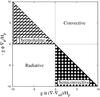 |
Fig. 1 Regions of different stability regimes for diffusion rates A = 0, D = 0.001, and F = 0. |
where ∇Rad is the temperature gradient that would be needed to transport the
whole flux by radiation, ρ is the density,
CP is the specific heat, K
is the radiative diffusive conductivity, and  is the
correlation between turbulent velocity and turbulent temperature excess given by
is the
correlation between turbulent velocity and turbulent temperature excess given by
 (3)where,
for simplicity, we have set
X = gα(∇ − ∇ad)/Hp
and
Y = gφ∇μ/Hp.
Our Eq. (3) differs from Grossman &
Taam’s Eq. (17) because we have fixed some sign errors present in the original expression.
It is worth mentioning that for realistic cases D ≫ A,
D ≫ F and D goes to zero.
(3)where,
for simplicity, we have set
X = gα(∇ − ∇ad)/Hp
and
Y = gφ∇μ/Hp.
Our Eq. (3) differs from Grossman &
Taam’s Eq. (17) because we have fixed some sign errors present in the original expression.
It is worth mentioning that for realistic cases D ≫ A,
D ≫ F and D goes to zero.
Equations (1) and (2) have to be solved simultaneously for σ and (∇ − ∇ad). The leading factor of Eq. (1) shows that σ = 0 is always a solution, but it corresponds to a stable equilibrium only if no other real and non-negative root exists. In general, the fluid will seek out the most turbulent equilibrium state; thus, if more than one root is positive, the system will evolve to the largest root, because the σ = 0 solution is unstable. Figure 1 shows the regions of different stability regimes for a realistic choice of the diffusion rates. Note the convective region with ∇ − ∇ad < 0 for which the standard mixing length approach (∇μ = 0) cannot provide mixing velocities and which have sometimes been misidentified with the thermohaline regime.
In the present work the mixing of nuclear species of mass fraction
Xi is performed by solving the diffusion
equation ![Mathematical equation: \begin{equation} {{\rm{d} X_i} \over {\rm{d}t}}= \left( {{\partial X_i}\over{\partial t}} \right)_\mathrm{nuc}+ {\partial\over{\partial M_r}} \left[ (4\pi r^2\rho)^2 D_\mathrm{c}{{\partial X_i}\over{\partial M_r}}\right] \end{equation}](/articles/aa/full_html/2011/09/aa17029-11/aa17029-11-eq42.png) (4)with
the diffusion coefficient Dc defined in terms of the turbulent
velocity σ and the mixing length l by (Weaver et al. 1978)
(4)with
the diffusion coefficient Dc defined in terms of the turbulent
velocity σ and the mixing length l by (Weaver et al. 1978)  (5)Appendix A contains a
few additional details about the procedure followed by us to solve GNA’s equations.
(5)Appendix A contains a
few additional details about the procedure followed by us to solve GNA’s equations.
3. An empirical scaling law for compositional transport by fingering convection
Although double-diffusive processes have been studied by several authors by means of
hydrodynamics codes (see, e.g., Merryfield 1995;
Biello 2001; Bascoul
2007; Zaussinger & Spruit 2010), it
was Traxler et al. (2011) who performed the first 3D
simulations to address the question of double-diffusive transport by fingering convection in
astrophysics. It is important to note that Traxler et al.
(2011) conducted their simulations at Pr ~ O(10-2), while the
true astrophysical regime occurs at Pr ~ O(10-6). Therefore, their
empirical scaling law relies on the validity of the asymptotic behavior suggested by their
results. They model a finger-unstable region using a local Cartesian frame
(x,y,z) oriented so that its vertical axis z has a
direction opposite to that of the gravitational acceleration. Also the Boussinesq
approximation is used and, consequently, it is assumed that low density, temperature, and
compositional perturbations  are
related by the following linearized equation
are
related by the following linearized equation  (6)where
ρ0 is a reference density,
(6)where
ρ0 is a reference density,
 , and
, and
 .
Expressing the velocity, temperature, and compositional fields as a background component,
plus a perturbation, it is found that
.
Expressing the velocity, temperature, and compositional fields as a background component,
plus a perturbation, it is found that
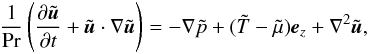
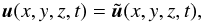 (7)
(7) (8)
(8) (9)with
T0(z) = z ∂T/∂z
and
μ0 = z ∂μ/∂z.
By scaling the time (t), the temperature, and the composition adequately by
means of the expected finger scale (see Traxler et al.
2011, for details), the final set of equations to solve turns out to be
(9)with
T0(z) = z ∂T/∂z
and
μ0 = z ∂μ/∂z.
By scaling the time (t), the temperature, and the composition adequately by
means of the expected finger scale (see Traxler et al.
2011, for details), the final set of equations to solve turns out to be
 (10)
(10) (11)
(11)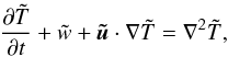 (12)
(12)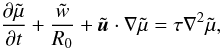 (13)where
 is
the z component of
is
the z component of  ,
Pr the Prandtl number,
,
Pr the Prandtl number,  the
nondimensional pressure perturbation from hydrostatic equilibrium,
R0 = (∇ − ∇ad)/∇μ and
τ = κμ/κT,
with κμ the compositional diffusivity (see
below) and κT the thermal diffusivity given by
the
nondimensional pressure perturbation from hydrostatic equilibrium,
R0 = (∇ − ∇ad)/∇μ and
τ = κμ/κT,
with κμ the compositional diffusivity (see
below) and κT the thermal diffusivity given by
 (14)In this last equation,
a stands for the radiation density constant, c is the
speed of light and κ the Rosseland mean opacity.
(14)In this last equation,
a stands for the radiation density constant, c is the
speed of light and κ the Rosseland mean opacity.
Traxler et al. (2011) solved Eqs. (10–13) in a triply periodic box of size (Lx,Ly,Lz) and carried out simulations for moderately low values of the Prandtl number and diffusivity ratio of order O(10-2).
As a result of numerical experiments, it turns out that the turbulent compositional
transport by fingering convection follows a simple law for the diffusion coefficient, namely
 (15)where
r = (R0 − 1)/(τ-1 − 1)
and ν is the total viscosity given by the sum of the molecular and
radiative viscosities (Denissenkov 2010)
(15)where
r = (R0 − 1)/(τ-1 − 1)
and ν is the total viscosity given by the sum of the molecular and
radiative viscosities (Denissenkov 2010)
 (16)with
  (17)and
![Mathematical equation: \begin{equation} \nu_\mathrm{mol}\equiv \kappa_\mu =1.84 \times 10^{-17} (1+7 X)\frac{T^{5/2}}{\rho} \qquad [\mathrm{cm}^2~\mathrm{s}^{-1}], \label{eq:mol-viscosity} \end{equation}](/articles/aa/full_html/2011/09/aa17029-11/aa17029-11-eq83.png) (18)where
X is the hydrogen mass fraction. Based on the asymptotic behavior shown
by their results, Traxler et al. (2011) suggest the
possibility of applying Eq. (15) to the more
extreme astrophysical regime, provided Pr is of order τ.
(18)where
X is the hydrogen mass fraction. Based on the asymptotic behavior shown
by their results, Traxler et al. (2011) suggest the
possibility of applying Eq. (15) to the more
extreme astrophysical regime, provided Pr is of order τ.
4. Numerical simulations
To study the effects of thermohaline instability in low-mass giant stars, we performed simulations using a 1D evolution code (LPCODE, Althaus et al. 2005) incorporating GNA’s convection theory to compute the mixing rates of the different stability regimes defined by this formalism. In our numerical experiments, we adopted the following choice for the parameters: A = 0, F = 0, D = 3K/(ρCPl2), α = 1, φ = 1, and l = 1.35 (approximately equivalent to a mixing length parameter of 1.61 in the usual Kippenhahn & Weigert 1990 prescription), and implemented the same nuclear reaction network as described at length in Althaus et al. (2005).
We computed stellar models of 0.9 M⊙, 1.3 M⊙, and 1.6 M⊙, each one with three different initial metallicities, namely Z = 3.17 × 10⁻⁴, 1 × 10⁻³, and 6.32 × 10⁻³, and let them evolve from the main sequence until after the luminosity bump. For each model, we paid special attention to the detailed stellar structure of the region between the HBS and the base of the convective envelope, contrasting the situation given before the star enters the luminosity bump region and after that stage of its evolution. The results obtained in all cases were qualitatively very similar, thus we show here just one case, namely the 0.9 M⊙, Z = 1 × 10⁻³ model, which is representative of what happens to the others. Figure 2 shows the abundance profiles of some elements and the mean molecular weight gradient for the 0.9 M⊙, Z = 1 × 10⁻³ model, before and after the luminosity bump. Before the luminosity bump (lefthand panel in Fig. 2), the mean molecular weight gradient ∇μ shows two peaks, corresponding to the hydrogen-burning shell (left peak) approaching the molecular weight discontinuity (right peak) left behind by the first dredge-up. When the hydrogen-burning shell reaches the discontinuity, the reaction 3He(3He, 2p)4He produces a molecular weight inversion in the external tail of the HBS, destabilizing the region and producing thermohaline convection. The destabilized zone (shown by plus signs in the righthand panel of Fig. 2) never reaches the convective envelope in our simulations, because both regions are separated by a radiative zone that prevents any change in the surface composition of the star. This result clearly differs from the main result presented by CZ07 when the slender-finger geometry of Ulrich (1972) was adopted. This should not come as a surprise because our assumption of a unique mixing length in GNA theory is far from a slender-finger geometry. In fact, our results are consistent with those of CZ07 when blobs, rather than slender fingers, are assumed. As shown by CZ07, different blob/finger geometries can affect the diffusion coefficient by more than two orders of magnitude. In this connection, we performed additional simulations that artificially increase GNA’s diffusion coefficient of thermohaline unstable layers by a factor of 103 in order to test the eventual relation between the more rapid mixing rate and the surface abundance variations. Figure 3 shows the abundance profile of the same elements included in Fig. 2, as well as the run of the molecular weight gradient in the region comprised by the HBS and the base of the convective envelope, for this new experiment. Now the thermohaline zone expands outwards (in mass) occupying all the former radiative region that separated it from the convective envelope. The contact between both convective regions allows for the noncanonical extra mixing to take place, thus modifying the photospheric chemical composition after the luminosity bump.
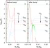 |
Fig. 2 Profiles of the abundances of H, 3He, 12C, 13C, 14N, 16O and of the mean molecular weight gradient ∇μ as a function of mass coordinate. The full line stands for ∇μ > 0 and the plus signs otherwise. Left and right panels correspond to the situation before and after the bump, respectively, for a 0.9 M⊙ model with 1 × 10⁻³. The abscissa ranges from the bottom of the hydrogen-burning shell to the base of the convective envelope. |
Given the contrast between the diffusion coefficients computed as given by the GNA and those reported by CZ07, we decided to perform further simulations that combine the GNA theory with other prescriptions used to estimate the diffusion coefficient. Only very few different prescriptions for the computation of the diffusion coefficient in thermohaline unstable regions exist in the literature. Ulrich (1972) was the first to derive an expression for the turbulent diffusivity produced by that instability, whereas Kippenhahn et al. (1980) extended previous works to the case of an imperfect gas. The linear theory used by these early works yield a solution for the diffusion coefficient that is proportional to the square of the unknown aspect ratio (length to diameter) of the fluid elements, which is still a matter of debate. Indeed, the diffusion coefficients may differ by about two orders of magnitude depending on the form factor adopted by different authors. Thus, the implementation of the linear theory has the drawback of containing a high intrinsic uncertainty. On the other hand, more recently, Traxler et al. (2011) successfully derived empirically determined transport laws for thermohaline unstable regions by means of 3D simulations performed at parameter values approaching those relevant for astrophysics. This represents an alternative and more physically sound approach that helps us to avoid the problems of the classical linear theory and that supplies an independent way to address the question of the actual role of mixing in thermohaline unstable regions.
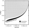 |
Fig. 4 Evolution of the region between the HBS and the convective envelope, when the prescription of Kippenhahn et al. (1980) is adopted to compute the diffusion coefficient in the thermohaline zone. The time interval spans from the instant when the stars luminosity reaches L ≈ 96 (i.e., before the luminosity bump) until L ≈ 1826, close to the top of the RGB. The figure corresponds to the 0.9 M⊙, Z = 1 × 10⁻³, model. |
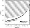 |
Fig. 5 Same as Fig. 4, but when the prescription of Traxler et al. (2011) is adopted to compute the diffusion coefficient in the thermohaline zone. The figure corresponds to the 0.9 M⊙, Z = 1 × 10⁻³, model. |
Since GNA convection theory may be implemented to determine the regime of energy transport
of any layer with the advantage of leaving the computation of the diffusion coefficient as
an independent task, which might adopt different prescriptions, we decided to study the
system’s response combining GNA formalism with two independent recipes. On the one hand, we
computed the thermohaline diffusion coefficient by means of the expression obtained by Kippenhahn et al. (1980)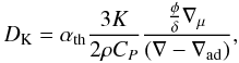 (19)where
αth is a efficiency parameter that depends on the geometry of
the fluid elements, ρ the density,
K = 4acT3/(3κρ)
the thermal conductivity, and
CP = (dq/dT)P
the specific heat capacity. We set αth = 2, which roughly
corresponds to the prescription of Kippenhahn et al.
(1980). On the other hand, we computed diffusion coefficients by adopting the Traxler et al. (2011) empirical law given by Eq. (15).
(19)where
αth is a efficiency parameter that depends on the geometry of
the fluid elements, ρ the density,
K = 4acT3/(3κρ)
the thermal conductivity, and
CP = (dq/dT)P
the specific heat capacity. We set αth = 2, which roughly
corresponds to the prescription of Kippenhahn et al.
(1980). On the other hand, we computed diffusion coefficients by adopting the Traxler et al. (2011) empirical law given by Eq. (15).
Thus, we performed a few additional simulations for the 0.9 M⊙, Z = 1 × 10⁻³, and 1 M⊙, Z = 0.02, sequences in order to investigate the response of the system when we solely vary the recipe to compute diffusion coefficients. Figure 4 shows the evolution of the thermohaline region along the RGB when the prescription of Kippenhahn et al. (1980) is adopted. The convective envelope never enters into contact with the thermohaline region. Consequently, for this model and mixing treatment, the photospheric abundances of the star remain constant throughout this phase. A similar behavior is shown by Fig. 5, corresponding to the implementation of the recipe of Traxler et al. (2011). In this case, the thermohaline zone is much narrower than before. We see in the next section that this fact is closely related to the magnitude of the diffusion coefficients computed using different prescriptions. Finally, it is worth noting that in our 1 M⊙ , Z = 0.02, sequence, we did not find any contact between the bottom of the convective envelope and the thermohaline region. This result is at variance with the simulations presented by Cantiello & Langer (2010), which shows that this contact occurred in 1 M⊙ mass stars even for the prescription of Kippenhahn et al. (1980) with αth = 2. We suspect that this different behavior may be due to the different microphysics assumed in both stellar codes.
5. Summary and discussion
We have studied the impact of thermohaline mixing in red giants close to the luminosity bump in the light of two nonstandard and physical sounding mixing prescriptions: the GNA and the Traxler et al. (2011) prescription. To the best of our knowledge, this is the first time that the empirically based thermohaline mixing prescription of Traxler et al. (2011) has been tested in the context of detailed evolutionary simulations. In the case of the double diffusive mixing length theory of Grossman et al. (1993), it allowed us to include thermohaline mixing in a consistent way with the other unstable regimes that are possible when ∇μ ≠ 0, selfconsistently solving the temperature gradients and turbulent mixing rates.
For the sake of completeness let us mention that in the case of GNA theory, we find the thermohaline mixing efficiency to be very similar to that of Kippenhahn et al. (1980). In fact our computations show that at almost all layers the value predicted by Grossman & Taam (1996) is DGNA ~ DKip/6, a difference that is just a consequence of different choices in the adimensional coefficients of both prescriptions. The similarities between these two prescriptions should not come as a surprise since the GNA theory is a sophisticated version of the mixing length theory, but it still relies on a very similar picture to the standard MLT, on which Kippenhahn et al. (1980) prescription is based. We consider our results as an actual validation of the GNA theory for the cases where the Kippenhahn et al. (1980) prescription is applicable.
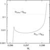 |
Fig. 6 Relation between diffusion coefficients computed using the prescriptions of Kippenhahn et al. (1980), DKip, Traxler et al. (2011), DTrx, and Grossman et al. (1993), DGNA. |
Both the Traxler et al. (2011) and Grossman et al. (1993) prescriptions have identified thermohaline mixing as developing in RGB stars close to the luminosity bump, in agreement with all previous works that have adopted more simplified approaches (Charbonnel & Zahn 2007; Cantiello & Langer 2010). However, in agreement with Denissenkov (2010) and Traxler et al. (2011), our full evolutionary calculations confirm that thermohaline mixing is not efficient enough for fingering convection to reach the bottom of the convective envelope of red giants. Thus, no changes in the surface chemical abundances of red giants are obtained when either Traxler et al. (2011) or Grossman et al. (1993) prescriptions are adopted. Interestingly enough, because the value of (∇ − ∇ad)/∇μ in the thermohaline zone is (∇ − ∇ad)/∇μ ~ 103... ~ 104, it falls in a regime in which the standard prescription of Kippenhahn et al. (1980) strongly overestimates the thermohaline mixing efficiency (see Fig. 3 of Traxler et al. 2011). As can be seen in Fig. 6, the standard prescription is ~100 to 1000 times more efficient than the empirical Traxler et al. (2011) law. However, we know from Cantiello & Langer (2010) that the standard prescription is still not enough to account for the surface abundances of RGBs. Thus, in order to allow contact between the thermohaline region and the convective envelope, the diffusion coefficient should be about four orders of magnitude higher than predicted by realistic thermohaline transport laws (Denissenkov 2010; Traxler et al. 2011). Since hydrodynamics codes have been shown to be consistent, yielding similar results between different implementations, they should be trusted in the physical regime studied (Pr ≥ 10-2), which due to computational limitations, is not the actual astrophysical regime (Pr ~ 10-6). While the prescriptions used here still rely on an asymptotic scaling, it seems unlikely that the diffusion coefficients are off by this much. Thus, we can conclude that thermohaline mixing alone is very unlikely to be the explanation for the chemical abundance anomalies of red giants.
Acknowledgments
We thank our referee for valuable comments and suggestions that helped us to improve the original version of this paper. We acknowledge financial support from PIP-112-200801-00904 by CONICET and PICT-2006-00504 by ANCyT.
References
- Althaus, L. G., Serenelli, A. M., Panei, J. A., at al. 2005, A&A, 435, 631 [NASA ADS] [CrossRef] [EDP Sciences] [Google Scholar]
- Bascoul, G. P. 2007, in IAU Symp. 239, ed. T. Kuroda, H. Sugama, R. Kanno, & M. Okamoto, 317 [Google Scholar]
- Biello, J. A. 2001, Ph.D. Thesis, The University of Chicago [Google Scholar]
- Cantiello, M., & Langer, N. 2010, A&A, 521, A9 [NASA ADS] [CrossRef] [EDP Sciences] [Google Scholar]
- Charbonnel, C. 1994, A&A, 282, 811 [NASA ADS] [Google Scholar]
- Charbonnel, C., & Do Nascimento, Jr., J. D. 1998, A&A, 336, 915 [NASA ADS] [Google Scholar]
- Charbonnel, C., & Lagarde, N. 2010, A&A, 522, A10 [NASA ADS] [CrossRef] [EDP Sciences] [MathSciNet] [PubMed] [Google Scholar]
- Charbonnel, C., & Zahn, J. 2007, A&A, 467, L15 (CZ07) [NASA ADS] [CrossRef] [EDP Sciences] [Google Scholar]
- Charbonnel, C., Brown, J. A., & Wallerstein, G. 1998, A&A, 332, 204 [NASA ADS] [Google Scholar]
- Denissenkov, P. A. 2010, ApJ, 723, 563 [NASA ADS] [CrossRef] [Google Scholar]
- Denissenkov, P. A., & Merryfield, W. J. 2011, ApJ, 727, L8 [NASA ADS] [CrossRef] [Google Scholar]
- Denissenkov, P. A., & Pinsonneault, M. 2008, ApJ, 684, 626 [NASA ADS] [CrossRef] [Google Scholar]
- Eggleton, P. P., Dearborn, D. S. P., & Lattanzio, J. C. 2006, Science, 314, 1580 [NASA ADS] [CrossRef] [PubMed] [Google Scholar]
- Geisler, D., Smith, V. V., Wallerstein, G., Gonzalez, G., & Charbonnel, C. 2005, AJ, 129, 1428 [NASA ADS] [CrossRef] [Google Scholar]
- Gilroy, K. K. 1989, ApJ, 347, 835 [NASA ADS] [CrossRef] [Google Scholar]
- Gilroy, K. K., & Brown, J. A. 1991, ApJ, 371, 578 [NASA ADS] [CrossRef] [Google Scholar]
- Gratton, R. G., Sneden, C., Carretta, E., & Bragaglia, A. 2000, A&A, 354, 169 [NASA ADS] [Google Scholar]
- Grossman, S. A., & Taam, R. E. 1996, MNRAS, 283, 1165 [NASA ADS] [CrossRef] [Google Scholar]
- Grossman, S. A., Narayan, R., & Arnett, D. 1993, ApJ, 407, 284 [NASA ADS] [CrossRef] [Google Scholar]
- Iben, Jr., I. 1967, ApJ, 147, 624 [NASA ADS] [CrossRef] [Google Scholar]
- Kippenhahn, R., & Weigert, A. 1990, Stellar Structure and Evolution (Berlin: Springer-Verlag) [Google Scholar]
- Kippenhahn, R., Ruschenplatt, G., & Thomas, H. 1980, A&A, 91, 175 [NASA ADS] [Google Scholar]
- Krishnamurti, R. 2003, J. Fluid Mech., 483, 287 [NASA ADS] [CrossRef] [Google Scholar]
- Luck, R. E. 1994, ApJS, 91, 309 [NASA ADS] [CrossRef] [Google Scholar]
- Merryfield, W. J. 1995, ApJ, 444, 318 [NASA ADS] [CrossRef] [Google Scholar]
- Recio-Blanco, A., & de Laverny, P. 2007, A&A, 461, L13 [NASA ADS] [CrossRef] [EDP Sciences] [Google Scholar]
- Shetrone, M. D. 2003, ApJ, 585, L45 [NASA ADS] [CrossRef] [Google Scholar]
- Smiljanic, R., Gauderon, R., North, P., et al. 2009, A&A, 502, 267 [NASA ADS] [CrossRef] [EDP Sciences] [Google Scholar]
- Smith, V. V., Hinkle, K. H., Cunha, K., et al. 2002, AJ, 124, 3241 [NASA ADS] [CrossRef] [Google Scholar]
- Spite, M., Cayrel, R., Hill, V., et al. 2006, A&A, 455, 291 [NASA ADS] [CrossRef] [EDP Sciences] [Google Scholar]
- Stancliffe, R. J. 2010, MNRAS, 403, 505 [NASA ADS] [CrossRef] [Google Scholar]
- Traxler, A., Garaud, P., & Stellmach, S. 2011, ApJ, 728, L29 [NASA ADS] [CrossRef] [Google Scholar]
- Ulrich, R. K. 1972, ApJ, 172, 165 [NASA ADS] [CrossRef] [Google Scholar]
- Weaver, T. A., Zimmerman, G. B., & Woosley, S. E. 1978, ApJ, 225, 1021 [NASA ADS] [CrossRef] [Google Scholar]
- Zaussinger, F., & Spruit, H. C. 2010 [arXiv:1012.5851] [Google Scholar]
Appendix A: Solving GNA’s equations
GNA theory of convection provides us with a set of equations that have to be solved in
order to find the values of the temperature gradient ∇ and the turbulent velocity
σ of the system in regions of different energy transport regimes. In
practice, this means we have to solve Eqs. (1) and (2) simultaneously.
Because it is impossible to express any of these variables in terms of the others, we
followed an iterative procedure and adopted the Newton-Raphson method to this end. To
avoid eventual numerical instabilities associated to the divergence of Eq. (3) when the denominator becomes small, we
elementarily transformed Eq. (2) by
multiplying it by that denominator. By rearranging the flux conservation equation we
obtain  (A.1)where we adopted the
following nomenclature
(A.1)where we adopted the
following nomenclature 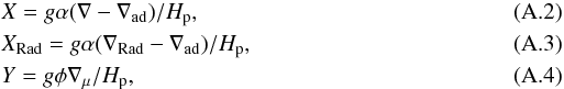 where
a1 and a2 are the coefficients
of the quadratic equation in X (i.e., ∇), which depend explicitly on the
turbulent velocity σ, the composition gradient
∇μ, and the total radiation gradient ∇Rad.
where
a1 and a2 are the coefficients
of the quadratic equation in X (i.e., ∇), which depend explicitly on the
turbulent velocity σ, the composition gradient
∇μ, and the total radiation gradient ∇Rad.
Thus, given a set of diffusion rates of heat (D), composition (F), and momentum (A), and once XRad and Y are known, we first determine whether the total radiation might be transported in a nonconvective way. If radiative transport is insufficient, convection has to carry some fraction of the energy flux, so we start the iterative procedure mentioned above. We adopt an initial (guess) value for X and solve Eq. (1) for σ. As stated before, the system will seek out the most turbulent equilibrium state, so we solve both cubic equations and pick up the largest positive root. The adopted values for X and σ are then introduced in Eq. (A.1), and the Newton-Raphson method is used to find the correction to be applied to X. By iterating this process it is possible to obtain the values of X and σ that satisfy Eqs. (1) and (A.1). Numerical experiments have shown that X = XRad is a good starting value for the Newton-Raphson process, while other choices resulted in the false roots found by the algorithm.
Finally, it is worth mentioning that factors in brackets in Eq. (1) are cubic in σ, and since both cubics are different, the conditions that separate the real roots’ region from the real one plus two complex conjugate roots region are also different. Despite this difference, for the stellar astrophysics case we find D ≫ A and D ≫ F, and both conditions tend to the same curve, making it unnecessary in practice to compute both limiting curves.
All Figures
|
Fig. 1 Regions of different stability regimes for diffusion rates A = 0, D = 0.001, and F = 0. |
| In the text | |
|
Fig. 2 Profiles of the abundances of H, 3He, 12C, 13C, 14N, 16O and of the mean molecular weight gradient ∇μ as a function of mass coordinate. The full line stands for ∇μ > 0 and the plus signs otherwise. Left and right panels correspond to the situation before and after the bump, respectively, for a 0.9 M⊙ model with 1 × 10⁻³. The abscissa ranges from the bottom of the hydrogen-burning shell to the base of the convective envelope. |
| In the text | |
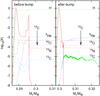 |
Fig. 3 Same as Fig. 2 for an artificially increased diffusion coefficient (see text). |
| In the text | |
|
Fig. 4 Evolution of the region between the HBS and the convective envelope, when the prescription of Kippenhahn et al. (1980) is adopted to compute the diffusion coefficient in the thermohaline zone. The time interval spans from the instant when the stars luminosity reaches L ≈ 96 (i.e., before the luminosity bump) until L ≈ 1826, close to the top of the RGB. The figure corresponds to the 0.9 M⊙, Z = 1 × 10⁻³, model. |
| In the text | |
|
Fig. 5 Same as Fig. 4, but when the prescription of Traxler et al. (2011) is adopted to compute the diffusion coefficient in the thermohaline zone. The figure corresponds to the 0.9 M⊙, Z = 1 × 10⁻³, model. |
| In the text | |
|
Fig. 6 Relation between diffusion coefficients computed using the prescriptions of Kippenhahn et al. (1980), DKip, Traxler et al. (2011), DTrx, and Grossman et al. (1993), DGNA. |
| In the text | |
Current usage metrics show cumulative count of Article Views (full-text article views including HTML views, PDF and ePub downloads, according to the available data) and Abstracts Views on Vision4Press platform.
Data correspond to usage on the plateform after 2015. The current usage metrics is available 48-96 hours after online publication and is updated daily on week days.
Initial download of the metrics may take a while.