| Issue |
A&A
Volume 533, September 2011
|
|
|---|---|---|
| Article Number | A95 | |
| Number of page(s) | 12 | |
| Section | The Sun | |
| DOI | https://doi.org/10.1051/0004-6361/201016300 | |
| Published online | 07 September 2011 | |
Twisted magnetic tubes with field aligned flow
I. Linear twist and uniform longitudinal field⋆
1
Departament de FísicaUniversitat de les Illes Balears,
07122
Palma de Mallorca,
Spain
e-mail: toni.diaz@uib.es, ramon.oliver@uib.es, dfsjlb0@uib.es
2
Centre for Plasma Astrophysics, Department of Mathematics,
Katholieke Universiteit Leuven, Celestijnenlaan 200B, 3001
Leuven,
Belgium
e-mail: roberto.soler@wis.kuleuven.be
Received:
13
December
2010
Accepted:
17
June
2011
Aims. We study the equilibrium and stability of twisted magnetic flux tubes with mass flows along the field lines. Then, we focus on the stability and oscillatory modes of magnetic tubes with uniform twist B0 = B0(r/p eϕ + ez) in a zero-β plasma, surrounded by a uniform, purely longitudinal field.
Methods. First we investigate the possible equilibriums, and then consider the linearised MHD equations and obtain a system of two first-order differential equations. These are solved numerically, while analytical approximations involving confluent hypergeometric functions are found in the thin tube limit. Finally, new appropriate boundary conditions are deduced and the outer solution considered (with the apparition of cut-off frequencies). We use this to derive a dispersion relation, from which the frequencies of the normal modes can be obtained.
Results. Regarding the equilibrium, the only value of the flow that satisfies the equations for this magnetic field configuration is a super-Alfvénic one. Then, we consider the normal modes of this configuration. The thin-tube approximation proves accurate for typical values, and it is used to prove that the equilibrium is unstable, unless the pitch is large. The stability criteria for twisted tubes are significantly lowered.
Conclusions. The twisted tube is subject to the kink instability unless the pitch is very high, since the Lundquist criterion is significantly lowered. This is caused by the requirement of having a magnetic Mach number greater than 1, so the magnetic pressure balances the magnetic tension and fluid inertia. This type of instability might be observed in some solar atmospheric structures, like surges.
Key words: Sun: oscillations / Sun: magnetic topology / Sun: corona
Appendix is available in electronic form at http://www.aanda.org
© ESO, 2011
1. Introduction
With the improvement of the observational capabilities in recent years with high spatial and temporal resolution, jets and flows are clearly observed in the solar atmosphere, such as in photospheric/chromospheric magnetic structures (Katsukawa et al. 2007; Shibata et al. 2007; de Pontieu et al. 2007; Nishizuka et al. 2008), coronal loops (Winebarger et al. 2002; Ofman & Wang 2008), prominences (Lin et al. 2003, 2005; Okamoto et al. 2007; Lin et al. 2009), or coronal holes (Cirtain et al. 2007; Scullion et al. 2009).
On the other hand, there is evidence of twisted magnetic fields in the solar atmosphere. Photospheric motions may stretch and twist anchored magnetic fields, which may lead to the consequent changes in topology in higher regions. The observed rotation of sunspots may lead to twisting of the magnetic tubes above active regions (Brown et al. 2003; Yan & Qu 2007; Kazachenko et al. 2009). Also newly emerged magnetic tubes are supposed to be twisted during the rising phase through the convection zone (Emonet & Moreno-Insertis 1996; Moreno-Insertis & Emonet 1996; Emonet & Moreno-Insertis 1998; Archontis et al. 2004; Murray & Hood 2008; Hood et al. 2009). Likewhise, some chromospheric surges show evidence of twisting fields and movement (Gu et al. 1994; Canfield et al. 1996; Jibben & Canfield 2004; Liu 2008; Liu et al. 2009). Therefore, solar magnetic tubes may have been twisted at photospheric, chromospheric, and coronal levels. Solar prominences are also supposed to be formed in a twisted magnetic field (Priest et al. 1989). However, not all works on prominence formation and equilibrium assume twisted fields, so the issue is still not clear today.
A flow-aligned magnetic field may stabilise sub-Alfvénic flows against the classical Kelvin-Helmholtz instability, while a transverse magnetic field seems to have no effect on the instability (Chandrasekhar 1961; Ferrari et al. 1981; Cohn 1983). Therefore, the magnetic field topology is crucial for the threshold of flow instability; namely, the twist of magnetic tubes may affect the instability properties of axial mass flows. Twisted magnetic tubes are also subject to the kink instability when the twist exceeds a critical value (Lundquist 1951; Hood & Priest 1979). In fact, Anzer (1968a,b) showed that all force-free fields without line-tying are unstable (regardless of whether they are smooth or have interfaces), but in the solar atmosphere the assumption of force-free fields is not always valid, so it remains important to investigate the instabilities in these models.
The magnetohydrodynamic modes of a twisted magnetic flux tube without flow can be used to study the threshold of the kink instability (Dungey & Loughhead 1954; Roberts 1956; Bennett et al. 1999; Carter & Erdélyi 2008; Soler et al. 2010). The effect of a monolithic flow along the axis has been considered by Zaqarashvili et al. (2010), who conclude that its effect is a correction on Lundquist’s stability criterion, although it can trigger the Kelvin-Helmholtz instability if the wavelength is large enough. However, this axial flow simply drags the field lines along the axis (so its main effect is to Doppler-shift the frequencies), while in the observations it is often suggested that the flows are field aligned. Our aim is therefore to study this type of twisted equilibrium configurations with plasma flowing along the field lines and to obtain their stability regimes.
2. Equilibrium configurations
We consider a magnetic flux tube with radius a and density ρl embedded in a uniform field environment with density ρe. The magnetic field inside the tube is helicoidal, while outside the magnetic field is uniform and directed along the z-axis. Both ρl and ρe are supposed to be homogeneous. The cylindrical coordinate system (r,φ,z) is used. No mass flow is present outside the tube, so the surrounding coronal medium is considered to be uniformly magnetised (Beẑ is a constant), uniform (ρe constant), and lacking mass flow at the equilibrium.
To study this equilibrium we use the set of ideal MHD equations, since no dissipative
effects are taken into account. These equations are  (1)plus
the solenoidal condition ∇·B = 0. We have labelled the gas
pressure as pg to avoid confusion with other parameters that
appear later in this paper.
(1)plus
the solenoidal condition ∇·B = 0. We have labelled the gas
pressure as pg to avoid confusion with other parameters that
appear later in this paper.
Next we describe the equilibrium quantities (labelled 0). The equilibrium magnetic field
inside the tube has the form  (2)with
B0 = Bl, representing a twisted
flux tube. We keep B0 in this section to point out that these
relations can be applied to other configurations. Assuming therefore that the equilibrium
gas pressure at the boundary is the same inside and outside, the continuity of the total
pressure across the tube boundary gives
(2)with
B0 = Bl, representing a twisted
flux tube. We keep B0 in this section to point out that these
relations can be applied to other configurations. Assuming therefore that the equilibrium
gas pressure at the boundary is the same inside and outside, the continuity of the total
pressure across the tube boundary gives
![\begin{equation} B_{\rm e}=B_{\rm l} \sqrt{ \left[\alpha(a)\right]^2+\left[\gamma(a) \right]^2}. \end{equation}](/articles/aa/full_html/2011/09/aa16300-10/aa16300-10-eq15.png) (3)This choice of equilibrium
magnetic field assumes that there is a current sheet at the loop boundary.
(3)This choice of equilibrium
magnetic field assumes that there is a current sheet at the loop boundary.
Moreover, the plasma is assumed to flow along the field lines inside the magnetic tube,
so we prescribe the equilibrium velocity field as  (4)with
v0 = vl for our model with a
twisted field inside the tube, and again we keep v0 in this
section. Notice that
v0 × B0 = 0,
∇·B0 = 0, and
∇·v0 = 0, satisfying the induction equation, the
solenoidal condition and the mass continuity equation, respectively. However, the equation
of motion,
(4)with
v0 = vl for our model with a
twisted field inside the tube, and again we keep v0 in this
section. Notice that
v0 × B0 = 0,
∇·B0 = 0, and
∇·v0 = 0, satisfying the induction equation, the
solenoidal condition and the mass continuity equation, respectively. However, the equation
of motion, 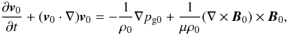 (5)indicates that the
magnetic field is not force-free inside the tube, since there is an electric current
(5)indicates that the
magnetic field is not force-free inside the tube, since there is an electric current
 (6)so the Lorentz force must
be balanced by the advection and pressure terms. Assuming a stationary equilibrium and using
some vector identities, we cast Eq. (5) as
(6)so the Lorentz force must
be balanced by the advection and pressure terms. Assuming a stationary equilibrium and using
some vector identities, we cast Eq. (5) as
 (7)This
equation can also be written to introduce the total pressure,
pT0 = B0·B0/(2μ) + pg0,
(7)This
equation can also be written to introduce the total pressure,
pT0 = B0·B0/(2μ) + pg0,
 (8)Since
B0 and
v0 are parallel vectors, this means that the
pressure terms must be balanced by a tension force that is lessened by a
factor
(8)Since
B0 and
v0 are parallel vectors, this means that the
pressure terms must be balanced by a tension force that is lessened by a
factor  (with the Alfvén speed squared defined as
  ) because of the field-aligned
flow.
) because of the field-aligned
flow.
Finally, using our equilibrium magnetic field and velocity (Eqs. (2) and (4)), this yields a differential equation for the radial
functions α(r)
and γ(r), ![\begin{eqnarray} \label{ab_rel}&& \caosq \left[ \alpha (r) \frac{{\rm d} \alpha (r)}{{\rm d}r} + \gamma (r) \frac{{\rm d} \gamma (r)}{{\rm d}r} \right] \nonumber \\ && \qquad\qquad + \,\left(\caosq-v_0^2 \right) \frac{[\alpha(r)]^2}{r} - \frac{1}{\ro} \frac{{\rm d} \, \pgo (r)}{{\rm d}r} =0. \end{eqnarray}](/articles/aa/full_html/2011/09/aa16300-10/aa16300-10-eq34.png) (9)This
gives a relation between both r-dependent components of the magnetic field
and the equilibrium gas pressure: two are freely chosen, and Eq. (9) then gives the other dependence so that the
equilibrium relations are satisfied.
(9)This
gives a relation between both r-dependent components of the magnetic field
and the equilibrium gas pressure: two are freely chosen, and Eq. (9) then gives the other dependence so that the
equilibrium relations are satisfied.
In this paper we are interested in studying a tube with uniform pressure, so the equilibrium pressure does not depend on the radial coordinate, so pg0 = pgl = pge = const. Then, Eq. (9) gives a relation between both components of the equilibrium magnetic field, so we just can freely choose one of them.
2.1. Uniform axial field
A particular case of the previous section is to assume that
γ(r) = 1, so the axial components of both the
equilibrium velocity and magnetic field are uniform. Under these conditions, Eq. (9) gives
 (10)The non-trivial
solution is (with Ka an arbitrary constant)
(10)The non-trivial
solution is (with Ka an arbitrary constant)  (11)Following Eq. (11), there is a family of solutions whose
radial dependence is prescribed by the relation between the magnitudes of the equilibrium
velocity and magnetic field. Sub-Alfvénic flows
(v0 < cA0) are only in
balance if the radial dependence diverges when r → 0, but super-Alfvénic
flows (v0 > cA0) lead to
finite values at the tube axis. The particular case
(11)Following Eq. (11), there is a family of solutions whose
radial dependence is prescribed by the relation between the magnitudes of the equilibrium
velocity and magnetic field. Sub-Alfvénic flows
(v0 < cA0) are only in
balance if the radial dependence diverges when r → 0, but super-Alfvénic
flows (v0 > cA0) lead to
finite values at the tube axis. The particular case
 leads to a linear profile (uniform twist of the flux tube and
j0 = 2pB0/μ ez),
similar to the one considered by Zaqarashvili et al.
(2010), but with the plasma flowing along the field lines instead of a purely
axially monolithic flow. This is also an extension of the classical study in Chandrasekhar (1961), which is performed assuming the
plasma is incompressible.
leads to a linear profile (uniform twist of the flux tube and
j0 = 2pB0/μ ez),
similar to the one considered by Zaqarashvili et al.
(2010), but with the plasma flowing along the field lines instead of a purely
axially monolithic flow. This is also an extension of the classical study in Chandrasekhar (1961), which is performed assuming the
plasma is incompressible.
3. Wave equations
3.1. Wave equation inside the magnetic tube for uniform twist
The equations governing the dynamics of the plasma for small perturbations (labelled 1)
from the equilibrium state are obtained from the linearisation of Eqs. (1), namely 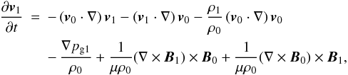 (12)
(12) (13)
(13) (14)
(14) (15)cs
being the sound speed. We also consider a situation in which the plasma beta is low, and
then the gradient of the gas pressure perturbation in Eq. (12) can be neglected in front of the magnetic and advection terms,
so Eq. (15) is not needed and we are
left with seven unknown functions, namely the components of the perturbed magnetic field
and the perturbed velocity and the perturbed density.
(15)cs
being the sound speed. We also consider a situation in which the plasma beta is low, and
then the gradient of the gas pressure perturbation in Eq. (12) can be neglected in front of the magnetic and advection terms,
so Eq. (15) is not needed and we are
left with seven unknown functions, namely the components of the perturbed magnetic field
and the perturbed velocity and the perturbed density.
The system of equations in Eqs. (12)−(15) are a generalisation for field-aligned flows of the well-known equations for twisted tubes, which are recovered if we set v0 = 0 (Hain & Lüst 1958; Appert et al. 1974). The equation for the perturbed density (Eq. (14)) needs to be considered with the rest, since the perturbed density now appears in the equation of motion (Eq. (12)).
Next, we assume a simple dependence for the equilibrium,
α(r) = r/p, which
satisfies Eq. (11) if
Ka = 1/p, with p the
pitch of the magnetic field, so 2πp is the longitudinal distance between
consecutive turns in the twisted flux tube. Then,
 (16)so the flow must be
super-Alfvénic to satisfy the motion equation. This equilibrium magnetic field,
B0 = Bl(0,r/p,1),
is the same as the one in Zaqarashvili et al.
(2010), but here the flow is field-aligned instead of being axis-oriented. The
equilibrium condition across the tube surface is then
(16)so the flow must be
super-Alfvénic to satisfy the motion equation. This equilibrium magnetic field,
B0 = Bl(0,r/p,1),
is the same as the one in Zaqarashvili et al.
(2010), but here the flow is field-aligned instead of being axis-oriented. The
equilibrium condition across the tube surface is then
 .
.
As the unperturbed parameters only depend on the r coordinate, the
perturbations can be Fourier-analysed with
exp [i(mφ + kz − ωt)] .
It is convenient to non-dimensionalise the perturbed quantities as
 (17)Then,
the wave equations can be cast as
(17)Then,
the wave equations can be cast as 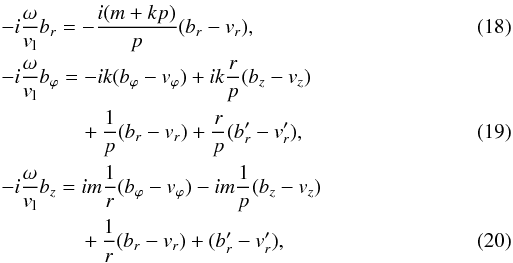
![\begin{eqnarray} && -i \frac{\omega}{v_{\rm l}} v_r = \frac{-1}{2 p} \left[\frac{4 r d}{p} + 3 b_\varphi -4 v_\varphi + r b_\varphi'+ p v_\varphi' \right. \nonumber \\[-1mm] && \qquad\qquad \left. \rule{0mm}{5mm} - \, i (m+kp) (b_r + 2 v_r) \right], \\[-1mm] && -i \frac{\omega}{v_{\rm l}} v_\varphi = \frac{i}{2 p r} \left[ r k p b_\varphi - 2 i r (b_r -2 v_r) \right. \nonumber \\ && \qquad\qquad \left. - \, 2m p v_z - 2 (m +kp) v_\varphi \right], \\[-1mm] && -i \frac{\omega}{v_{\rm l}} v_z = \frac{-i}{2 p} \left[ k r b_\varphi -m b_z + 2 (m+ kp) v_z \right], \end{eqnarray}](/articles/aa/full_html/2011/09/aa16300-10/aa16300-10-eq64.png)
![\begin{eqnarray} -i \frac{\omega}{v_{\rm l}} d &=& -\frac{i}{p r} \left[ (m+kp) r d + pm v_\varphi \right. \nonumber \\ && \left. - \, i (v_r+i k r v_z + r v'_r)\right]. \end{eqnarray}](/articles/aa/full_html/2011/09/aa16300-10/aa16300-10-eq65.png) (24)Next
we non-dimensionalise the variables as
(24)Next
we non-dimensionalise the variables as
 (25)with
the frequency including the factor vlk.
(25)with
the frequency including the factor vlk.
We can reduce the system to two first-order differential equations after some algebra,
![\begin{eqnarray} && d = \frac {P}{s} \frac{m v_\varphi+s v_z + i v_r + i s v'_r}{m+P(\Omega-1)}, \\[-1mm] && b_r = \frac{m+P}{m- P(\Omega-1)} v_r, \\ && v_z = \frac {-s b_\varphi + m b_z} {2(m-P(\Omega-1))}, \\[-1mm] && v_\varphi = - \frac{P (s b_\varphi-m b_z)}{2 s \left\{m-P(\Omega-1)\right\}} + \frac{i (m +P -2 P \Omega) v_r} {\left\{m-P(\Omega-1)\right\}^2}, \\ && b_\varphi = b_z \left[m^2 (s^2-P^2) + 2s^2P^2 (\Omega-1)^2 \right. \nonumber \\[-1mm] && \qquad - \, \left. -m P (P^2-3 s^2+4s^2\Omega ) \right] /\left[s \left(2m^2P+3mP^2 \right. \right. \nonumber \\[-1mm] && \qquad + \, \left. \left. P^3-ms^2-Ps^2-4mP^2\Omega \right) \right] + v_r \left[2 i (m+P)(m \right. \nonumber \\ && \qquad + \, \left.P-2P\Omega) \right]/ \left[(m+P-P \Omega) \left( 2m^2P+3mP^2 \right. \right. \nonumber \\[-1mm] && \qquad + \, \left. \left. P^3-ms^2-Ps^2-4mP^2\Omega \right) \right]. \end{eqnarray}](/articles/aa/full_html/2011/09/aa16300-10/aa16300-10-eq68.png) This
gives the following set of differential equations for the two remaining unknown radial
functions bz
and vr:
This
gives the following set of differential equations for the two remaining unknown radial
functions bz
and vr: 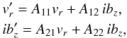 (31)where
{Aij} are algebraic real coefficients
depending on the parameters P, m and the radial
coordinate d (see the Appendix). Both variables have a phase shift
of π/4 for stable modes because of the i factor
in Eqs. (31).
(31)where
{Aij} are algebraic real coefficients
depending on the parameters P, m and the radial
coordinate d (see the Appendix). Both variables have a phase shift
of π/4 for stable modes because of the i factor
in Eqs. (31).
These two first-order differential equations can be transformed into one second-order
linear differential equation for vr with
non-constant coefficients, 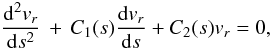 (32)
(32) (33)The
expressions of these coefficients in terms of the equilibrium parameters are given in the
Appendix. Both coefficients are quotients of polynomials of high order
in s; hence, the resulting differential equation is very difficult to
solve analytically, and numerical methods may prove useful to obtain its solutions.
In fact, Eq. (33) is similar to the
Hain-Lüst equation (Hain & Lüst 1958) for
twisted tubes without flow, but instead Eq. (33) is valid in a tube filled with uniform twist, low-beta plasma and a field
aligned flow.
(33)The
expressions of these coefficients in terms of the equilibrium parameters are given in the
Appendix. Both coefficients are quotients of polynomials of high order
in s; hence, the resulting differential equation is very difficult to
solve analytically, and numerical methods may prove useful to obtain its solutions.
In fact, Eq. (33) is similar to the
Hain-Lüst equation (Hain & Lüst 1958) for
twisted tubes without flow, but instead Eq. (33) is valid in a tube filled with uniform twist, low-beta plasma and a field
aligned flow.
It is interesting to check the singularities of this equation, since they provide
information about the solution. In addition to a singularity as s → ∞,
Eq. (32) is singular if ![\begin{eqnarray} \label{singul1} && s^2(s^2+P^2)(m+P-P \Omega) \left[m^2+2mP(1-2\Omega) \right.\nonumber \\ && \qquad\qquad \left.+P^2(1-4\Omega+2\Omega^2)\right]=0, \end{eqnarray}](/articles/aa/full_html/2011/09/aa16300-10/aa16300-10-eq82.png) (34)which
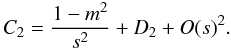
are the zeroes of the denominator of the coefficient C2
(Eq. (A.6)). The solutions of Eq. (34) give three frequencies near which infinite
modes are clustered (also called bands),
(34)which
are the zeroes of the denominator of the coefficient C2
(Eq. (A.6)). The solutions of Eq. (34) give three frequencies near which infinite
modes are clustered (also called bands), 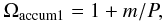 (35)
(35) (36)and
the position of additional singular points to infinity and 0,
(36)and
the position of additional singular points to infinity and 0,  (37)or
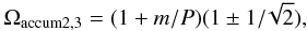
 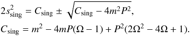 (38)These
additional singular points only appear if Ω > Ωaccum2 or
Ω < Ωaccum3 and for high values of s outside the
tube, so they are not relevant for our analysis.
(38)These
additional singular points only appear if Ω > Ωaccum2 or
Ω < Ωaccum3 and for high values of s outside the
tube, so they are not relevant for our analysis.
The position of the first band (Eq. (35))
can be related to the location of mode’s rational surfaces, which for a typical force-free
field are found when the axial wavenumber satisfies
 (39)with no dependence
on position in our equilibrium choice. Then,
ωaccum1 = (1 + m/(kp)) kvl
represents this accumulation point about which the band is centred. The second and third
bands (Eq. (36)) are similar to this one,
but related to the Alfvén frequency being close to the Doppler-shifted frequency, since in
our choice of equilibrium with uniform twist
(39)with no dependence
on position in our equilibrium choice. Then,
ωaccum1 = (1 + m/(kp)) kvl
represents this accumulation point about which the band is centred. The second and third
bands (Eq. (36)) are similar to this one,
but related to the Alfvén frequency being close to the Doppler-shifted frequency, since in
our choice of equilibrium with uniform twist  ,
so ωaccum2,3 = [1 + m/(kp)] k (vl ± cAl).
These bands are similar to those found in Zaqarashvili
et al. (2010).
,
so ωaccum2,3 = [1 + m/(kp)] k (vl ± cAl).
These bands are similar to those found in Zaqarashvili
et al. (2010).
3.2. Solution outside the flux tube
So far, we have derived a differential equation for the perturbed velocity inside the twisted flux tube (Eq. (32)), but to obtain solutions we need to consider the boundary conditions at the tube boundary r = a.
First of all, the solution outside the flux tube is relatively simple, since the outside
plasma is uniform and permeated by a constant magnetic
field Be. In these conditions a Bessel equation can be
obtained for the total pressure perturbation (Edwin
& Roberts 1983; Cally 1986; Díaz et al. 2002) after Fourier-analysing all the
variables except r,
 (40)(
(40)( ), with the radial perturbed
velocity related with the total pressure perturbation as
), with the radial perturbed
velocity related with the total pressure perturbation as
 (41)The solution for
r > a can be written as
(41)The solution for
r > a can be written as 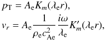 (42)with
 and
Ae and arbitrary constant. In our non-dimensional units
and
Ae and arbitrary constant. In our non-dimensional units
 (43)
(43) (44)
(44) (45)There is another
important point to consider: the presence of the external magnetic
field Be has the appearance of a cut-off frequency as a
consequence, since λe must be real to have an evanescent
solution for r → ∞. This condition gives the value of the cut-off
frequency
(45)There is another
important point to consider: the presence of the external magnetic
field Be has the appearance of a cut-off frequency as a
consequence, since λe must be real to have an evanescent
solution for r → ∞. This condition gives the value of the cut-off
frequency 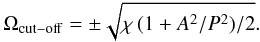 (46)Finally, there is an
interesting limit that is relevant to some solar atmospheric structures: high-density
ratio χ. In coronal loops this ratio is above unity, but can be much
higher in other structures, for example in prominences of typically
χ ≈ 100. We thus consider χ ≫ 1, so the external Alfvén
speed cAe in Eq. (44) increases. Then λe/k ≈ 1, the
cut-off frequency (Eq. (46)) becomes high,
and Eq. (43) can be simplified to
(46)Finally, there is an
interesting limit that is relevant to some solar atmospheric structures: high-density
ratio χ. In coronal loops this ratio is above unity, but can be much
higher in other structures, for example in prominences of typically
χ ≈ 100. We thus consider χ ≫ 1, so the external Alfvén
speed cAe in Eq. (44) increases. Then λe/k ≈ 1, the
cut-off frequency (Eq. (46)) becomes high,
and Eq. (43) can be simplified to
 (47)which for
A ≪ 1 gives
(47)which for
A ≪ 1 gives 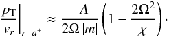 (48)
(48)
3.3. Boundary conditions (uniform twist)
Finally, we need boundary conditions to match these outer solutions to the inner ones.
The first one is the continuity of the normal component of the Lagrangian displacement,
and this condition is not modified by the presence of twist or flows. The second condition
is the continuity of the total pressure perturbation for untwisted tubes, but for twisted
tubes there are extra terms involving the equilibrium magnetic field azimuthal component
(Dungey & Loughhead 1954; Roberts 1956; Bennett
et al. 1999). However, in our model there are other extra terms coming from the
presence of non-uniform flows. The conditions must be imposed on the Lagrangian total
pressure, which is (Goedbloed 1983; Goedbloed & Poedts 2004; Goedbloed et al. 2010)
![\begin{equation} \left[ \vec{B}_0 \cdot \vec{B}_1 + \hat{n} \cdot \vec{\xi} \,\, \hat{n} \cdot \nabla ( \vec{B}_0 \cdot \vec{B}_0 /2) \right]=0. \end{equation}](/articles/aa/full_html/2011/09/aa16300-10/aa16300-10-eq117.png) (49)We use the convention
of denoting
[a] = a2 − a1
as the jump in the quantity a across the boundary, the subscripts 1 and 2
indicating the values on either side. Our boundary is
r = a, so
(49)We use the convention
of denoting
[a] = a2 − a1
as the jump in the quantity a across the boundary, the subscripts 1 and 2
indicating the values on either side. Our boundary is
r = a, so  and this equation becomes
 ![\begin{equation} \left[ \vec{B}_0 \cdot \vec{B}_1 + \xi_r \frac{\partial}{\partial r} ( \vec{B}_0 \cdot \vec{B}_0 /2) \right]=0. \end{equation}](/articles/aa/full_html/2011/09/aa16300-10/aa16300-10-eq120.png) (50)Using the equilibrium
condition (Eq. (8)), we obtain
(50)Using the equilibrium
condition (Eq. (8)), we obtain
![\begin{equation} \left[ \pt - (1-v_0^2/\casq) \frac{\xi_r B_\varphi^2}{\mu r} \right]=0, \end{equation}](/articles/aa/full_html/2011/09/aa16300-10/aa16300-10-eq121.png) (51)which with our choice of
constant z-component in the equilibrium magnetic field and uniform twist,
becomes
(51)which with our choice of
constant z-component in the equilibrium magnetic field and uniform twist,
becomes ![\begin{equation} [\xi_r]=0, \,\, \left[\pt + \frac{B_\varphi^2}{\mu r} \, \xi_r \right]=0, \label{bc} \end{equation}](/articles/aa/full_html/2011/09/aa16300-10/aa16300-10-eq122.png) (52)with a plus sign
in the term of the displacement.
(52)with a plus sign
in the term of the displacement.
We need to relate the displacement to the perturbed velocity, which is not trivial in a
flowing plasma. Following Goossens et al. (1992);
Goedbloed & Poedts (2004); Goedbloed et al. (2010), after neglecting non-linear
terms the relation is  (53)which using Eq. (4) gives
 (54)The
quantity
ωd = v0αm/r + v0kγ = v0(1 − m/p)
is the Doppler shift in frequency. Hence, in our variables the radial components of the
perturbed velocity and the displacement are related as
(54)The
quantity
ωd = v0αm/r + v0kγ = v0(1 − m/p)
is the Doppler shift in frequency. Hence, in our variables the radial components of the
perturbed velocity and the displacement are related as
 (55)In terms of our
functions, the total pressure perturbation inside the tube can be written as
(55)In terms of our
functions, the total pressure perturbation inside the tube can be written as ![\begin{eqnarray} && \pt - \frac{B_\varphi^2}{\mu r} \frac{v_r}{i (\omega-\omega_{\rm d})} = - i \rl v_{\rm l}^2 \frac{E_1 v_r + E_2 b_z}{D_{\rm bc1}} \nonumber \\ && D_{\rm bc1} = 2 P (m+P-P \Omega ) \left[2 m^2 P + (3-4 \Omega) m P^2 \right. \nonumber \\ && \qquad\quad \left. + \, (1-4\Omega+2\Omega^2) P^3- (m+P) s^2 \right]. \label{bc_coefs} \end{eqnarray}](/articles/aa/full_html/2011/09/aa16300-10/aa16300-10-eq127.png) (56)The
expressions of the coefficients E1 and
E2 are given in the Appendix.
(56)The
expressions of the coefficients E1 and
E2 are given in the Appendix.
As a result, we have the solution outside the flux tube and the matching conditions, so we can numerically solve the differential equation. However, we also need to impose another condition: regularity at r → 0, which implies that pT(r = 0) = 0. Then we can integrate from r = r0 to r = a, where r0 is a small number, chosen to avoid numerical instabilities at r = 0. Next we apply the boundary conditions in Eq. (52), to obtain the value of the constant Ae in Eq. (42), and then we use the second boundary condition to obtain the frequencies of the stationary modes of this model using a shooting and matching numerical scheme.
3.4. Thin tube limit
In many cases in the solar atmosphere we are dealing with thin tubes, that is, tubes whose length is much more longer than their width. Some approximations may exploit this condition to obtain analytical approximations. In our problem, the relevant parameter is A, whose order of magnitude is generally around 10-2.
Taking this into account, we can use the Taylor expansion of the coefficients in
Eq. (32) for s ≪ 1 and
m ≠ 0,  (57)
(57) (58)Again, the
expressions of the coefficients D1
and D2 are given in the Appendix. Notice
that D2 still has the three singularities that lead to the
accumulation frequencies and bands (Eqs. (35), (36)), but not the singular
points in Eq. (37), since they only appear
for large s. If we take the first-order approximation, Eq. (32) is written as
(58)Again, the
expressions of the coefficients D1
and D2 are given in the Appendix. Notice
that D2 still has the three singularities that lead to the
accumulation frequencies and bands (Eqs. (35), (36)), but not the singular
points in Eq. (37), since they only appear
for large s. If we take the first-order approximation, Eq. (32) is written as
 (59)whose solution is
 (60)with
K1 and K2 arbitrary constants.
Since we expect the solutions to be regular as s → 0, we demand that
K1 = 0. Then for kink modes (| m| = 1)
this gives vr ≈ const.,
while for fluting modes (| m| ≥ 2) this gives
vr ≈ 0, confirming the boundary
conditions in Sect. 3.3. The sausage mode
(m = 0) is a special case, so is considered in the next section.
(60)with
K1 and K2 arbitrary constants.
Since we expect the solutions to be regular as s → 0, we demand that
K1 = 0. Then for kink modes (| m| = 1)
this gives vr ≈ const.,
while for fluting modes (| m| ≥ 2) this gives
vr ≈ 0, confirming the boundary
conditions in Sect. 3.3. The sausage mode
(m = 0) is a special case, so is considered in the next section.
We can now use the following order in the expansions in Eqs. (57), (58), so the differential equation is cast as 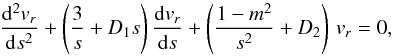 (61)which is a form of
the Whittaker differential equation, whose solutions can be written in terms of confluent
hypergeometric functions F(a,b;x). The
general solution of Eq. (61) for
m ≠ 0 is
(61)which is a form of
the Whittaker differential equation, whose solutions can be written in terms of confluent
hypergeometric functions F(a,b;x). The
general solution of Eq. (61) for
m ≠ 0 is  (62)Again,
the condition of having regular solutions as s → 0 is satisfied if we
impose K3 = 0 (m > 0) or
K4 = 0 (m < 0). The solution for
m > 0 is therefore
(62)Again,
the condition of having regular solutions as s → 0 is satisfied if we
impose K3 = 0 (m > 0) or
K4 = 0 (m < 0). The solution for
m > 0 is therefore  (63)and
the equivalent one for m < 0.
(63)and
the equivalent one for m < 0.
We can expand this expression further for small s to gain insight into
the solution
 (64)Thus,
we recover the first-order expansion results and obtain a correction.
(64)Thus,
we recover the first-order expansion results and obtain a correction.
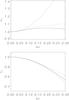 |
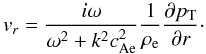
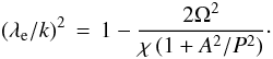
Fig. 1 Spatial plots of χr (arbitrary units) inside the magnetic tube for m = 1. The solid line is the numerical solution of Eq. (32), the dotted line represents the thin tube approximation in terms of confluent hypergeometric functions (Eq. (63)), and the dashed line its first-order expansion (Eq. (64)). The upper panel is calculated with P = 0.5 and Ω = 1.5, while the lower panel is done with P = 2.0 and Ω = 4.0. |
We test these approximations by plotting the numerical solution of the system, the solution in terms of the confluent hypergeometric functions (Eq. (63)) and its first-order series expansion (Eq. (64)) for a typical set of values for the parameters. This is seen in Fig. 1. For s < 0.1 both approximations are quite accurate, so the approximations can be used in the range appropriate to solar atmospheric conditions, while for higher values of s the analytical approximation is no longer valid. Also, for high values of P, the range where the analytical solution is accurate increases, but at the same time, this range decreases for high values of Ω.
Next, we need to write the expressions for the boundary conditions (Eq. (52)) in terms
of vr and its derivative ![\begin{eqnarray} \label{bc_seran} && \pt - \frac{B_\varphi^2}{\mu r} \frac{v_r}{i (\omega-\omega_{\rm d})} = - i \rl v_{\rm l}^2 s \frac{E_3 v_r + E_4 v_r'}{D_{\rm bc2}}, \nonumber \\ && D_{\rm bc2} = 2 P (m+P-P \Omega ) \left[m^2 (P^2+s^2) \right. \nonumber \\ && \qquad\quad \left. + \, 4 m P s^2 (\Omega-1) - s^2 P^2 (1-4\Omega+2\Omega^2) + s^4\right], \end{eqnarray}](/articles/aa/full_html/2011/09/aa16300-10/aa16300-10-eq170.png) (65)with
the expressions of the coefficients given in the Appendix. Finally, using Eqs. (43) and (63) we can obtain a dispersion relation
(65)with
the expressions of the coefficients given in the Appendix. Finally, using Eqs. (43) and (63) we can obtain a dispersion relation 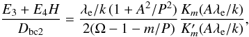 (66)with
![\begin{eqnarray} H&=& \left. \frac{1}{v_r} \frac{\partial v_r}{\partial s} \right|_{s=A}=- \frac{[(m-1)D_1 + D_2] A}{2 (m+1)} \nonumber \\ && \times \, \frac{F\left(\frac{(m+1)D_1+D_2}{2 D_1}, m+2; - \frac{D_1 A^2}{2} \right)}{F\left(\frac{(m-1)D_1+D_2}{2 D_1}, m+1; - \frac{D_1 A^2}{2} \right)} + \frac{m-1}{A}\cdot \end{eqnarray}](/articles/aa/full_html/2011/09/aa16300-10/aa16300-10-eq172.png) (67)Focusing
on the kink m = 1 mode this expression gives
(67)Focusing
on the kink m = 1 mode this expression gives
 (68)We can have an
approximation to this dispersion relation expanding in series for a
small A. Using the properties of the confluent hypergeometric functions
and the approximation in Eq. (48) for the
external solution, the first-order approximation of Eq. (66) for m ≠ 0 gives a sixth-order algebraic equation
for Ω
(68)We can have an
approximation to this dispersion relation expanding in series for a
small A. Using the properties of the confluent hypergeometric functions
and the approximation in Eq. (48) for the
external solution, the first-order approximation of Eq. (66) for m ≠ 0 gives a sixth-order algebraic equation
for Ω  (69)whose coefficients
are given in the Appendix. There is no simple form for expressing the roots of this
equation, but it may provide a fast way to compute the solutions, even the ones with
complex frequencies that may appear as solutions of this algebraic equation.
(69)whose coefficients
are given in the Appendix. There is no simple form for expressing the roots of this
equation, but it may provide a fast way to compute the solutions, even the ones with
complex frequencies that may appear as solutions of this algebraic equation.
3.4.1. Sausage modes
We have so far investigated the modes with m ≠ 0. However, the modes
that satisfy m = 0 (also called sausage modes) must be dealt with
separately. We follow the same procedure by expanding the coefficients in Eq. (32) for s ≪ 1 and
m = 0,  (70)
(70) (71)Our differential
equation is written in the first-order approximation as
(71)Our differential
equation is written in the first-order approximation as
 (72)whose solution is
 (73)with
K10 and K20 as arbitrary
constants. Since we expect the solutions to be regular as s → 0, we
require that K20 = 0. Now we have
vr ≈ K10s,
which is different from the m ≠ 0 modes. In fact, to obtain these
solutions numerically the condition that needs to be imposed is
v′(s) = const. This is somewhat
expected, since even for a straight magnetic flux tube without twist or flow, the
sausage modes behave differently as r → 0.
(73)with
K10 and K20 as arbitrary
constants. Since we expect the solutions to be regular as s → 0, we
require that K20 = 0. Now we have
vr ≈ K10s,
which is different from the m ≠ 0 modes. In fact, to obtain these
solutions numerically the condition that needs to be imposed is
v′(s) = const. This is somewhat
expected, since even for a straight magnetic flux tube without twist or flow, the
sausage modes behave differently as r → 0.
We can now use the following order in the expansions in Eqs. (70), (71), so the differential equation is cast as  (74)which is a form
of the Whittaker differential equation, whose solutions can be written in terms of
confluent hypergeometric
functions F(a,b;x). The regular
solution as s → 0 is
(74)which is a form
of the Whittaker differential equation, whose solutions can be written in terms of
confluent hypergeometric
functions F(a,b;x). The regular
solution as s → 0 is  (75)We can expand this
expression further for small s to gain insight into the solution
(75)We can expand this
expression further for small s to gain insight into the solution
 (76)again,
recovering the first order expansion results and obtaining a correction.
(76)again,
recovering the first order expansion results and obtaining a correction.
Finally, we can write the dispersion relation for the sausage modes as Eq. (66), but with
 (77)
(77)
4. Stability of the model
Once we have discussed the differential equations and boundary conditions necessary for
solving them, we can look for their solutions. First of all, we need to consider which
parameters are relevant to our study. After non-dimensionalising the equations we are left
with a set of parameters {m,P,A,χ,Ω} , since the flow speed and the
equilibrium magnetic field are related in our equilibrium by
 . We first focus on
the kink mode (m = 1), since it is the easiest mode to detect in
observations and the one that leads to unstable modes in similar equilibrium configurations.
. We first focus on
the kink mode (m = 1), since it is the easiest mode to detect in
observations and the one that leads to unstable modes in similar equilibrium configurations.
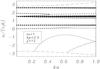 |
Fig. 2 Dispersion diagram (Eq. (66)) plotting the non-dimensional frequency ω/(vlk) against the non-dimensional tube radius ka for the values of the parameters shown in the legend. Stable solutions are plotted in solid lines, while unstable solutions are plotted in dotted lines. The numerical solution of the system in Eq. (31) has been overplotted as diamonds. The dashed lines represent the external cut-off frequencies (Eq. (46)). |
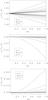 |
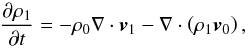
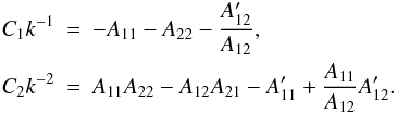
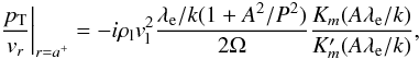
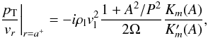
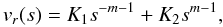
Fig. 3 Zoom of the dispersion diagram of Fig. 2 (Eq. (31)) near the bands for the values of the parameters shown in the legend. Only the first ten modes farther from each accumulation frequency have been plotted in each panel. The upper panel is centred on the first band (Eq. (35)), the central panel is around the second band (positive sign of Eq. (36)), and the lower one is around the third band (negative sign of Eq. (36)). The values of the accumulation frequencies have been overplotted as a dashed line. |
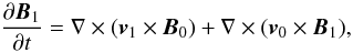
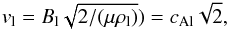
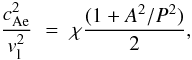
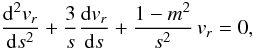
We first study the dependence of the frequency on the tube radius ka (Fig. 2) for a given set of the rest of parameters. The thin-tube approximation shows the right behaviour even for ka > 0.1, although the negative frequencies are not obtained correctly. There is a rich array of modes, and we can distinguish the three bands whose frequencies are clustered around the accumulation frequencies in Eqs. (35), (36), which for these parameters correspond to Ωaccum1 = 1.63, Ωaccum2 = 2.77, and Ωaccum3 = 0.48. Only a few modes in each band have been represented. A zoom of the dispersion diagram around the bands is shown in Fig. 3, where we can see that the first band is symmetric with respect to Ωaccum1, while the second and third bands only have modes on one side of their accumulation frequency and are much more clustered. The spatial shape of these modes, shown in Fig. 4, contains an increasing number of wiggles near the tube boundary as the mode frequency approaches the accumulation frequency. This can be understood better by checking previous results: in a twisted tube without flow (Bennett et al. 1999), the solution can be expressed in terms of Bessel functions, and the band appears when the argument becomes large, allowing many extrema in the interior of the tube boundary. In our model we can see a similar behaviour in the thin-tube limit: for the hypergeometric functions in Eq. (63) the D2 coefficient becomes large as Ω → Ωaccum (Eq. (A.10)), so many extrema are added to the eigenfunction inside the tube as we approach the accumulation frequency (Fig. 4).
We can also see an instability being triggered in Fig. 2: two modes become complex at the bifurcation point at ka = 0.42, ω/(vlk) = 1.79. These modes are the first ones in each band, with a single maximum in r = 0 and no minimum.
 |
Fig. 4 Spatial plots of vr (arbitrary units) for the values in the legend. Only the five modes whose frequency is farthest from the accumulation frequency have been represented (Fig. 3, upper panel), each mode with a different linestyle. The vertical dashed line is the position of the tube boundary. |
The dependence on the parameters can be sumarised as follows: modifying the density ratio χ affects the frequencies slightly, but raising it also increases the cut-off frequency (Eq. (46)), allowing more modes to become trapped. Even one or more bands might become leaky for low values of χ. Raising the tube radius ka expands the bands where infinite modes are clustered and eventually can lead to destabilisations, while changing the pitch kp modifies the position of the bands.
We next concentrate on the unstable modes (Fig. 5). As ka is decreased these modes merge, and beyond the bifurcation point they become unstable: now their frequencies have a complex part. For this particular choice of parameters the model would therefore be unstable for ka < Acrit = 0.152. In accordance with Zaqarashvili et al. (2010), the instability threshold is no longer located in Ω = 0 (as in Bennett et al. 1999) because of the presence of a flow, but in this case the exact value of the threshold is calculated numerically. Solving the comparatively simple Eq. (69) for the thin tube gives quite accurate results.
 |
Fig. 5 Dispersion diagram plotting ω/(vlk) against kp for the values of the parameters shown in the legend. The upper panel represents the real part of the frequencies and the lower panel the imaginary part. Stable solutions are plotted in solid lines, while unstable solutions are plotted in dotted lines. The dashed line represents the external cut-off frequency (Eq. (46)), while the dot-dashed lines represent the position of the accumulation frequencies of each band (Eqs. (35), (36)). Only the modes that go through the bifurcations have been plotted. The results of the algebraic equation in Eq. (69) have been overplotted as dots. |
 |
Fig. 6 Stability diagram (χ = 15) for different values of the azimuthal
number m. The dashed line represents the threshold without flow
(Dungey & Loughhead 1954), while the
dotted line represents the threshold with a monolithic axial flow with
|
Finally, we represent the threshold of the instability (Fig. 6). We can see that the stability region is very limited, and for modes with
kp < 1 the tube is unstable unless ka ≪ 1. We can
compare it with the results of a twisted tube without flow (Dungey & Loughhead 1954; Roberts
1956; Bennett et al. 1999) and with a twisted
tube with monolithic axial flow (Zaqarashvili et al.
2010) to check that the stability threshold on the corrected Lundquist’s
instability criterion, which in our variables is
 (78)and this type of flow
lowers it substantially. The m = 1 mode is the first mode that becomes
unstable as ka is increased.
(78)and this type of flow
lowers it substantially. The m = 1 mode is the first mode that becomes
unstable as ka is increased.
5. Conclusions
We have studied the equilibrium properties of twisted magnetic flux tubes with flows along the field lines and found the relations between the equilibrium quantities that must be satisfied. One of the main differences with equilibriums studied in previous works is that the pressure must be balanced by a lessened tension force due to the advection term in the equation of motion, but otherwise the equilibriums are similar to those of twisted flux tubes without flow (see for example Priest 1982).
We then focused on one particular case, a tube with uniform twist across the radial
coordinate,
B0 = Bl(0,r/p,1),
since it is a particularly interesting case that has been considered in many studies. We
found that the flow velocity must be super-Alfvénic to satisfy the equilibrium relations,
 . Although these
high values can be matched with a few observations, it is interesting to point out that is
the only equilibrium in a zero-beta plasma that has a uniform twist and a field-aligned
plasma velocity.
. Although these
high values can be matched with a few observations, it is interesting to point out that is
the only equilibrium in a zero-beta plasma that has a uniform twist and a field-aligned
plasma velocity.
Next we studied the stability of this equilibrium by obtaining the normal modes, both numerically by solving the system of ordinary differential equations obtained from the linearised MHD system and obtaining analytical approximations in the thin tube limit, which led to confluent hypergeometric functions. One needs to be careful deriving the appropriate boundary conditions in this situation, since the continuity of the perturbed velocity and the total pressure are no longer valid. The analytical approximation is accurate enough if the tube radius is small. Compared with the case of monolithic axial flow (Zaqarashvili et al. 2010), there are three bands of infinite modes clustered around the Doppler-shifted frequency with the flow speed and the flow plus and minus the Alfvén speed. This appears even with our configuration of the flow, which does not lead to a simple frequency Doppler shift in the differential equations.
Finally, we investigated the stability of the equilibrium and found that the stability
region is significantly lowered. This contradicts the results in Chandrasekhar (1961) for the incompressible case. If we compute the ratio
between the magnetic energy and the total energy (Eq. (297), Chapter XII) we obtain
 (79)which is below 1/2,
and thus stable in the incompressible range following their results, but unstable in the
compressible range if ka is not very small. Another important difference
with previous results is that the marginal stability does not occur when
ω = 0, as in Dungey & Loughhead
(1954); Roberts (1956); Bennett et al. (1999), or at the Doppler-shifted
frequency, as in Zaqarashvili et al. (2010). This
kink instability of the model may be caused by the large magnitude of the flow needed to
assure that the uniform twisted tube is in equilibrium. It is therefore necessary to relax
some assumptions in the equilibrium to study equilibriums with sub-Alfvénic flows, either by
having a radial dependence for the magnetic field or taking the plasma pressure into
account. The investigation of these cases is left for later work.
(79)which is below 1/2,
and thus stable in the incompressible range following their results, but unstable in the
compressible range if ka is not very small. Another important difference
with previous results is that the marginal stability does not occur when
ω = 0, as in Dungey & Loughhead
(1954); Roberts (1956); Bennett et al. (1999), or at the Doppler-shifted
frequency, as in Zaqarashvili et al. (2010). This
kink instability of the model may be caused by the large magnitude of the flow needed to
assure that the uniform twisted tube is in equilibrium. It is therefore necessary to relax
some assumptions in the equilibrium to study equilibriums with sub-Alfvénic flows, either by
having a radial dependence for the magnetic field or taking the plasma pressure into
account. The investigation of these cases is left for later work.
This instability in super-Alfvénic twisted flows may play a relevant role in chromospheric surges. This plasma eruptions may reach propagating speeds of 50−200 km s-1, over the typical Alfvén speed in the lower layers of the atmosphere. Moreover, some surges fall back or are ejected as CMEs, but sometimes they are disrupted (Jibben & Canfield 2004; Liu 2008). For example, with the data in Jibben & Canfield (2004) for NOAAA AR 7117 surge in 1992 March 28, the axial velocity is vl = 150 km s-1, while a rotational velocity of Ωrot ≈ 10-3 radian s-1 leads to a pitch of p = vl/Ωrot ≈ 1.5 × 10⁵ km. We can estimate from the panels that the surge width is about 20′′, so we obtain a radius of a ≈ 14 000 km, which gives a/p = A/P ≈ 0.1. This line has been overplotted in the stability diagram in Fig. 7. Thus, this surge would be unstable under perturbations with P < 1.7, that is, for k ≈ 10-5 km-1 and smaller wavenumbers. Unfortunately, it is difficult to estimate the axial wavelength of the perturbation observationally, but it is possible that this kind of instability may cause the mentioned disruption, along with this surge and other observed ones. In Liu (2008) it is suggested that the so classified diffuse surges are spread because of the overlying magnetic configuration in which the surge is propagating, but this disruption could also be caused by some instability. Again, we need to refine our analytical work to allow further comparisons with observations, but the different stability regimes could explain the behaviour of super-Alfvénic surges and the disruption of some observed surges.
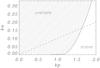 |
Fig. 7 Stability diagram for m = 1, with the unstable region filled with dots. The dashed line represents the equilibrium models that satisfy the observational parameters in Jibben & Canfield (2004). |
Finally, it is worth remarking that the unstable regions are larger in this model than in previous ones, mainly because the high value of the magnetic Mach number needed in the equilibrium to have a field-aligned flow with a uniform longitudinal speed. However, it is also known in twisted force-free fields that photospheric line-tying is an essential ingredient to stabilise the loops (Raadu 1972; Hood & Priest 1979). Other important ingredients are the current layer at the interface, which in this work has been addressed in the boundary conditions, here, other effects might be important, such as dissipation by resistivity and resonant absorption. However, these effects are expected to have little influence on the stability of the modes. Also, other equilibrium configurations need to be addressed: for example, Eq. (11) for other profiles of B0ϕ and different values of the magnetic Mach number, or Eq. (9) for tubes without uniform longitudinal component B0z. The stability analysis of these modes is left for later work on this topic.
Online material
Appendix A: Coefficients in the equations
The coefficients that appear in Eq. (31) can be computed with the help of a symbolic computation program. These
coefficients turn out to be rather cumbersome quotients of polynomic expressions in our
model with uniform twist, ![\appendix \setcounter{section}{1} \begin{eqnarray} && A_{11} = \left[(m+P) s^2-P^2 (m+P (2 (\Omega -2) \Omega \right. \nonumber \\ && \qquad \left. + \, 1))\right]/\left[P s \left(2 m^2+P (3-4 \Omega ) m+P^2 (2 (\Omega -2) \Omega \right. \right. \nonumber \\ && \qquad \left. \left. + \, 1)\right)-(m+P) s^3\right], \end{eqnarray}](/articles/aa/full_html/2011/09/aa16300-10/aa16300-10-eq224.png) (A.1)
(A.1)![\appendix \setcounter{section}{1} \begin{eqnarray} && A_{12} = \left[(m+P-P \Omega ) \left(s^4-\left(m^2-4 P (\Omega -1) m \right. \right. \right.\nonumber \\ && \qquad \left. \left. \left. + \, P^2 (2 (\Omega -2) \Omega +1)\right) s^2+m^2 P^2\right)\right]/\left[P s^2 \left(2 m^2 \right. \right.\nonumber \\ && \qquad \left.\left. + \, P (3-4 \Omega ) m+P^2 (2 (\Omega -2) \Omega +1)\right) \right.\nonumber \\ && \qquad \left.-\, (m+P) s^4\right], \end{eqnarray}](/articles/aa/full_html/2011/09/aa16300-10/aa16300-10-eq225.png) (A.2)
(A.2)![\appendix \setcounter{section}{1} \begin{eqnarray} && A_{21} = \left[4 P^2 m^8-4 P \left((10 \Omega -7) P^2+s^2\right) m^7 \right.\nonumber \\ && \qquad \left.+\, \left((4 \Omega (41 \Omega -62)+85) P^4+\left(s^2 (32 \Omega -26)-4\right) P^2 \right.\right.\nonumber \\ && \qquad \left. \left. + \, s^4\right) m^6+2 P \left((\Omega (4 (111-46 \Omega ) \Omega -327)+73) P^4 \right.\right.\nonumber \\ && \qquad \left. \left. + \, 2 \left(-3 (\Omega (8 \Omega -15)+6) s^2+10 \Omega -6\right) P^2+12 s^2 \right.\right.\nonumber \\ && \qquad \left. \left. - \, 3 s^4 (\Omega -1)\right) m^5+\left((\Omega -1) (\Omega (4 \Omega (125 \Omega -299) \right.\right.\nonumber \\ && \qquad \left. \left. - \, 795)-155) P^6+2 \left((\Omega (\Omega (72 \Omega -229)+210)\right.\right.\right.\nonumber \\ && \qquad \left. \left. \left.- \, 55) s^2+2 (50-39 \Omega ) \Omega -30\right) P^4+s^2 \left(s^2 (\Omega (11 \Omega \right.\right.\right.\nonumber \\ && \qquad \left. \left. \left. - \, 30)+15)-112 (\Omega -1)\right) P^2-8 s^4\right) m^4 \right.\nonumber \\ && \qquad \left. - \, 4 P \left((\Omega (\Omega (\Omega (\Omega (106 \Omega -471)+778)-591)+205) \right. \right. \nonumber \\ && \qquad \left. \left. - \, 26) P^6+\left((\Omega (\Omega (\Omega (29 \Omega -140)+218)-130) \right. \right. \right. \nonumber \\ && \qquad \left. \left. \left. - \, 25) s^2+4 (\Omega ((39-19 \Omega ) \Omega -25)+5)\right) P^4 \right. \right. \nonumber \\ && \qquad \left. \left. + \, s^2 \left((2 \Omega -1) ((\Omega -5) \Omega +5) s^2-46 \Omega ^2+107 \Omega \right. \right. \right. \nonumber \\ && \qquad \left. \left. \left. - \, 52\right) P^2+s^4 (8-5 \Omega )\right) m^3+P^2 \left((2 (\Omega -2) \Omega \right. \right. \nonumber \\ && \qquad \left. \left. + \, 1) (2 \Omega (\Omega (\Omega (55 \Omega -196)+244) -124)+43) P^6 \right. \right. \nonumber \\ && \qquad \left. \left. + \, 2 \left((2 \Omega -3) \left(2 \Omega \left(\Omega \left(6 \Omega^2-34 \Omega +51\right)-27\right)+9\right) s^2 \right. \right. \right.\nonumber \\ && \qquad \left. \left.\left.+ \, 4 \Omega (50-3 \Omega (\Omega (13 \Omega -38)+39))-30\right) P^4 \right. \right.\nonumber \\ && \qquad \left. \left. + \, s^2 \left((2 \Omega (\Omega ((\Omega -12) \Omega +33)-30)+15) s^2 \right. \right.\right.\nonumber \\ && \qquad \left. \left. \left. - \, 4 \Omega (8 \Omega (4 \Omega -17)+153)+192\right) P^2-4 s^4 (\Omega (2 \Omega \right.\right.\nonumber \\ && \qquad \left. \left. - \, 15)+12)\right) m^2-2 P^3 \left((\Omega -1) (2 \Omega -1) (4 \Omega \right.\right.\nonumber \\ && \qquad \left. \left. - \, 5) (2 (\Omega -2) \Omega +1)^2 P^6+2 (\Omega -1) \left(s^2 (2 (\Omega -2) \Omega \right.\right.\right.\nonumber \\ && \qquad \left. \left.\left. + \, 1) (\Omega ((\Omega -9) \Omega +13)-4)-2 (2 \Omega (\Omega (\Omega (10 \Omega \right.\right.\right.\nonumber \\ && \qquad \left. \left.\left. - \, 29)+28)-11)+3)\right) P^4-s^2 \left((\Omega -1) (2 \Omega ((\Omega \right.\right.\right.\nonumber \\ && \qquad \left. \left.\left. - \, 5) \Omega +6)-3) s^2+2 (\Omega (2 \Omega (4 (\Omega -8) \Omega +67)-97) \right.\right.\right.\nonumber \\ && \qquad \left. \left.\left. + \, 22)\right) P^2+2 s^4 (\Omega (4 \Omega -15)+8)\right) m \right.\nonumber \\ && \qquad \left. + \, P^4 \left((\Omega -1)^2 (2 (\Omega -2) \Omega +1)^3 P^6-2 (\Omega -1)^2 (2 (\Omega \right.\right.\nonumber \\ && \qquad \left. \left. - \, 2) \Omega +1) \left(2 (\Omega -2) \Omega s^2+s^2+8 (\Omega -1) \Omega +2\right) P^4 \right.\right.\nonumber \\ && \qquad \left. \left. + \, s^2 \left(s^2+\Omega \left(-6 s^2+\left(s^2+16\right) \Omega (2 (\Omega -4) \Omega +11) \right.\right.\right.\right.\nonumber \\ && \qquad \left. \left. \left.\left. - \, 92\right)+16\right) P^2-4 s^4 (\Omega (2 \Omega -5)+2)\right)\right]/\left[\left(P^2 \right.\right.\nonumber \\ && \qquad \left. \left. + \, s^2\right) (m+P-P \Omega)^3 \left(m^2+P (2-4 \Omega) m \right.\right.\nonumber\\ && \qquad \left. \left. + \, P^2 (2 (\Omega -2) \Omega +1)\right) \left(P \left(2 m^2+P (3-4 \Omega ) m \right.\right.\right.\nonumber \\ && \qquad \left. \left. \left. + \, P^2 (2 (\Omega -2) \Omega +1)\right)-(m+P) s^2\right)\right], \end{eqnarray}](/articles/aa/full_html/2011/09/aa16300-10/aa16300-10-eq226.png) (A.3)
(A.3)![\appendix \setcounter{section}{1} \begin{eqnarray} && A_{22} = \left[6 (m+P) s^4-2 P \left(9 m^2+2 P (7-9 \Omega ) m \right.\right.\nonumber \\ && \qquad \left. \left. + \, P^2 (8 (\Omega -2) \Omega +5)\right) s^2-2 m P^3 (m+P \right.\nonumber \\ && \qquad \left. - \, 2 P \Omega )\right]/\left[ s \left(P^2+s^2\right) \left(P \left(2 m^2+P (3-4 \Omega ) m \right.\right.\right.\nonumber \\ && \qquad \left. \left.\left. + \, P^2 (2 (\Omega -2) \Omega +1)\right)-(m+P) s^2\right)\right]. \end{eqnarray}](/articles/aa/full_html/2011/09/aa16300-10/aa16300-10-eq227.png) (A.4)Next,
we can compute the coefficients in Eq. (33),
(A.4)Next,
we can compute the coefficients in Eq. (33), ![\appendix \setcounter{section}{1} \begin{eqnarray} && C_1 = \frac{9}{s} -\frac{8 P^2}{s(P^2+s^2)}+\left[2 m^2 P^2-2 s^4 \right]/ \left[(P^2-s^2) \right.\nonumber \\ && \qquad \left. + \, m^2+4 P s^2 (\Omega -1) m+s^2 \left(\left(-2 \Omega ^2+ 4 \Omega -1\right) P^2 \right. \right.\nonumber \\ && \qquad \left. \left. + \, s^2\right) s\right], \end{eqnarray}](/articles/aa/full_html/2011/09/aa16300-10/aa16300-10-eq228.png) (A.5)
(A.5)![\appendix \setcounter{section}{1} \begin{eqnarray} && C_2= -\left[-\left(P^2-s^2\right)^2 m^8+2 P \left(P^2-s^2\right) \left((3 \Omega -2) P^2 \right. \right.\nonumber \\ && \qquad \left. \left. +\, s^2 (6-7 \Omega )\right) m^7+\left(\left(-11 \Omega ^2+18 \Omega -6\right) P^6\right. \right.\nonumber \\ && \qquad \left. \left. +\, \left(2 \left(37 \Omega ^2-62 \Omega +23\right) s^2+1\right) P^4-s^2 \left(\left(79 \Omega ^2 \right. \right. \right. \right.\nonumber \\ && \qquad \left. \left. \left. \left. -\, 138 \Omega +58\right) s^2+2\right) P^2+2 s^6+s^4\right) m^6+2 P \left((\Omega \right. \right.\nonumber \\ && \qquad \left. \left. -\, 1) (\Omega (4 \Omega -7)+2) P^6+\left(2 (\Omega ((85-32 \Omega ) \Omega -68) \right. \right.\right.\nonumber \\ && \qquad \left. \left. \left. +\, 16) s^2-3 \Omega +2\right) P^4+s^2 \left((\Omega -1)(\Omega (116 \Omega -195) \right.\right.\right.\nonumber \\ && \qquad \left. \left.\left. +\, 70) s^2+10 \Omega -8\right) P^2+s^4 \left((8-10 \Omega ) s^2-7 \Omega \right.\right.\right.\nonumber \\ && \qquad \left. \left.\left. +\, 6\right)\right) m^5-\left((\Omega -1)^2 \left(2 \Omega ^2-4 \Omega +1\right) P^8-\left(2 \left(56 \Omega ^4 \right.\right.\right.\right.\nonumber \\ && \qquad \left. \left. \left. \left. -\, 208 \Omega ^3+266 \Omega ^2- 136 \Omega +23\right) s^2+11 \Omega ^2-18 \Omega \right.\right.\right.\nonumber \\ && \qquad \left.\left. \left. +\, 6\right) P^6+s^2 \left(\left(386 \Omega ^4-1416 \Omega ^3+1843 \Omega ^2-998 \Omega \right.\right.\right.\right.\nonumber \\ && \qquad \left.\left.\left. \left. +\, 186\right) s^2+60 \Omega ^2-68 \Omega +27\right) P^4-s^4 \left(2 \left(37 \Omega ^2 \right.\right.\right.\right.\nonumber \\ && \qquad \left. \left. \left. \left. -\, 62 \Omega +23\right) s^2+69 \Omega ^2-98 \Omega +56\right) P^2+s^6 \left(s^2\right.\right.\right.\nonumber \\ && \qquad \left. \left.\left. +\, 11\right)\right) m^4-2 P \left((\Omega -1) \left(2 (2 \Omega -1) (3 \Omega -4) (2 (\Omega \right.\right.\right.\nonumber \\ && \qquad \left.\left. \left. -\, 2) \Omega +1) s^2+\Omega (4 \Omega -7)+2\right) P^6 \right.\right.\nonumber \\ && \qquad \left. \left. +\, s^2 \left((\Omega (4 \Omega (\Omega ((221-47 \Omega ) \Omega -392)+325)-499)\right.\right.\right.\nonumber \\ && \qquad \left. \left. \left. +\, 70) s^2+\Omega \left(-28 \Omega ^2+46 \Omega -23\right)+6\right) P^4 \right.\right.\nonumber \\ && \qquad \left. \left. +\, s^4 \left(2 (\Omega (\Omega (32 \Omega -85)+68)-16) s^2+\Omega (\Omega (72 \Omega \right.\right.\right.\nonumber \\ && \qquad \left. \left.\left. -\, 131)+99)-38\right) P^2+s^6 \left((2-3 \Omega ) s^2-37 \Omega \right.\right.\right.\nonumber \\ && \qquad \left. \left. \left. +\, 34\right)\right) m^3+\left((\Omega -1)^2 (2 (\Omega -2) \Omega +1) \left(2 (2 (\Omega -2) \Omega \right.\right.\right.\nonumber \\ && \qquad \left. \left. \left. +\, 1) s^2+1\right) P^8 +s^2 \left(-(2 (\Omega -2) \Omega +1) (\Omega (\Omega (2 \Omega (53 \Omega \right.\right.\right.\nonumber \\ && \qquad \left. \left. \left. -\, 200)+535)-298)+58) s^2+\Omega (\Omega (2 (8-7 \Omega ) \Omega \right.\right.\right.\nonumber \\ && \qquad \left. \left. \left. +\, 17)-22)+4\right) P^6+s^4 \left(2 (2 \Omega (\Omega (4 \Omega (7 \Omega -26)\right.\right.\right.\nonumber \\ && \qquad \left. \left. \left. +\, 133)-68)+23) s^2+\Omega (\Omega (8 \Omega (15 \Omega -31)+141)\right.\right.\right.\nonumber \\ && \qquad \left. \left. \left. -\, 50)+21\right) P^4-s^6 \left((\Omega (11 \Omega -18)+6) s^2+3 \left(51 \Omega ^2\right.\right.\right.\right.\nonumber \\ && \qquad \left. \left. \left.\left. -\, 90 \Omega +38\right)\right) P^2+8 s^8\right) m^2+2 P s^2 \left((\Omega -1) (2 (\Omega \right.\right.\nonumber \\ && \qquad \left. \left. -\, 2) \Omega +1) \left((2(\Omega -2) \Omega +1) (\Omega (8 \Omega -15)+6) s^2\right.\right.\right.\nonumber \\ && \qquad \left. \left. \left. +\, (5-2 \Omega ) \Omega -2\right) P^6-2 s^2 (\Omega -1) \left((2 \Omega -1) (3 \Omega \right.\right.\right.\nonumber \\ && \qquad \left. \left. \left. -\, 4) (2 (\Omega -2) \Omega +1) s^2+(\Omega -1) \Omega (5 \Omega (2 \Omega +1)\right.\right.\right.\nonumber \\ && \qquad \left. \left. \left. -\, 24)-4\right) P^4+s^4 \left((\Omega -1) (\Omega (4 \Omega -7)+2) s^2\right.\right.\right.\nonumber \\ && \qquad \left. \left. \left. +\, \Omega (\Omega (52 \Omega -149)+129)-34\right) P^2+2 s^6 (4-5 \Omega )\right) m \right.\nonumber \\ && \qquad \left. +\, P^2 s^2 \left(-(\Omega (-2 (\Omega -3) \Omega -5)+1)^2 \left(s^2 (2 (\Omega -2) \Omega \right.\right.\right.\nonumber \\ && \qquad \left. \left. \left. +\, 1)-1\right) P^6+2 s^2 (\Omega -1)^2 (2 (\Omega - 2) \Omega \right.\right.\nonumber \\ && \qquad \left. \left. +\, 1) \left((2 (\Omega -2) \Omega +1) s^2+\Omega (\Omega +6)-3\right) P^4\right.\right.\nonumber \\ && \qquad \left. \left. -\, s^4 \left(s^2 (2 (\Omega -2) \Omega +1) (\Omega -1)^2+\Omega (11 \Omega (2 (\Omega \right.\right.\right.\nonumber \\ && \qquad \left. \left. \left. -\, 4) \Omega +11)-62)+11\right) P^2+4 s^6 (\Omega (2 \Omega -5)\right.\right.\nonumber \\ && \qquad \left. \left. +\, 2)\right) \rule{0mm}{4mm} \right] / \left[ \rule{0mm}{4mm} s^2 \left(P^2+ s^2\right) (m+P-P \Omega )^2 \left(m^2+P (2\right.\right.\nonumber \\ && \qquad \left. \left. -\, 4 \Omega ) m+P^2 \left(2 \Omega ^2-4 \Omega +1\right)\right) \left(\left(s^2-P^2\right) m^2 \right.\right.\nonumber \\ && \qquad \left. \left. -\, 4 P s^2 (\Omega -1) m+s^2 \left(P^2 \left(2 \Omega ^2-4 \Omega +1\right)\right.\right.\right.\nonumber \\ && \qquad \left. \left. \left. -\, s^2\right)\right) \rule{0mm}{4mm} \right]. \label{c2_coeff} \end{eqnarray}](/articles/aa/full_html/2011/09/aa16300-10/aa16300-10-eq229.png) (A.6)Then,
the coefficients that appear in the boundary conditions (Eq. (56)) are given by
(A.6)Then,
the coefficients that appear in the boundary conditions (Eq. (56)) are given by
![\appendix \setcounter{section}{1} \begin{equation} E_1 = -s \left[ (m+P-2P \Omega^2) P^2 + (m+P) s^2 \right], \end{equation}](/articles/aa/full_html/2011/09/aa16300-10/aa16300-10-eq230.png) (A.7)
(A.7)![\appendix \setcounter{section}{1} \begin{eqnarray} E_2 &=& (m+P-\Omega P) (P^2+s^2) \left[ m^2 + 2 m P (1-2 \Omega) \right.\nonumber \\ && \left. + \, P^2(1-4\Omega+2\Omega^2) \right]. \end{eqnarray}](/articles/aa/full_html/2011/09/aa16300-10/aa16300-10-eq231.png) (A.8)The
coefficients that appear in the thin tube limit for the differential equations
(Eqs. (57), (58)) can be cast as
(A.8)The
coefficients that appear in the thin tube limit for the differential equations
(Eqs. (57), (58)) can be cast as  (A.9)
(A.9)![\appendix \setcounter{section}{1} \begin{eqnarray} D_2&=& \left[2 m^8+12 P m^7-16 P \Omega m^7+29 P^2 m^6 \right.\nonumber \\ && \left. -\, 48 P^2 \Omega^2 m^6-80 P^2 \Omega m^6-2 m^6+36 P^3 m^5 \right.\nonumber \\ && \left. -\, 72 P^3 \Omega^3 m^5+192 P^3 \omega^2 m^5-12 P m^5-154 P^3 \Omega m^5\right.\nonumber \\ && \left. +\, 16 P \Omega m^5+24 P^4 m^4+58 P^4 \Omega^4 m^4-216 P^4 \omega^3 m^4 \right.\nonumber \\ && \left. -\, 10 P^2 m^4+277 P^4 \Omega^2 m^4-34 P^2 \Omega^2 m^4-142 P^4 \Omega m^4\right.\nonumber \\ && +\, \left. 24 P^2 \Omega m^4+8 P^5 m^3-24 P^5 \Omega^5 m^3+116 P^5 \Omega^4 m^3\right.\nonumber \\ && \left. +\, 16 P^3 m^3-208 P^5 \Omega^3 m^3+170 P^5 \omega^2 m^3\right.\nonumber \\ && \left. +\, 56 P^3 \Omega^2 m^3-62 P^5 \Omega m^3-72 P^3 \Omega m^3+P^6 m^2\right.\nonumber \\ && \left. +\, 4 P^6 \Omega ^6 m^2-24 P^6 \Omega^5 m^2+26 P^4 m^2+56 P^6 \Omega^4 m^2\right.\nonumber \\ && \left. -\, 40 P^4 \Omega^4 m^2-64 P^6 \Omega^3 m^2-184 P^4 \Omega^3 m^2\right.\nonumber \\ && \left. +\, 37 P^6 \Omega^2 m^2+272 P^4 \Omega^2 m^2-10 P^6 \Omega m^2\right.\nonumber \\ && \left. -\, 152 P^4 \Omega m^2+12 P^5 m-32 P^5 \Omega^5 m+160 P^5 \Omega^4 m\right.\nonumber \\ && \left. -\, 296 P^5 \Omega^3 m+248 P^5 \Omega^2 m-92 P^5 \Omega m+2 P^6\right.\nonumber \\ && \left. -\, 8 P^6 \Omega^6 -48 P^6 \Omega^5+112 P^6 \Omega^4-128 P^6 \Omega ^3\right.\nonumber \\ && \left. -\, 74 P^6 \Omega^2-20 P^6 \Omega \right] / \left[m^2 P^2 (m+P-P \Omega )^2 \left(m^2 \right.\right.\nonumber \\ && \left.\left. +\, 2 P m-4 P \Omega m+P^2+2 P^2 \Omega^2-4 P^2 \Omega \right)\right]. \label{d2coeff} \end{eqnarray}](/articles/aa/full_html/2011/09/aa16300-10/aa16300-10-eq233.png) (A.10)
(A.10)
The coefficients for the boundary conditions suitable for analytical solution
(Eq. 65), which also appear in the
dispersion relation (Eq. 66), are
![\appendix \setcounter{section}{1} \begin{equation} E_3= s \left[ s^4+2P^2s^2(1-2\Omega) + P^4(1-4\Omega+2\Omega^2) \right], \end{equation}](/articles/aa/full_html/2011/09/aa16300-10/aa16300-10-eq234.png) (A.11)
(A.11)![\appendix \setcounter{section}{1} \begin{eqnarray} E_4&=& s^2 (s^2+P^2) \left[(m+P)^2-4P (m+P) \right. \Omega \nonumber \\ && + \, \left. 2 P^2 \Omega^2 \right], \end{eqnarray}](/articles/aa/full_html/2011/09/aa16300-10/aa16300-10-eq235.png) (A.12)Finally,
the coefficients that appear on the sixth-order algebraic equation (Eq. 69) for m > 0 are
(A.12)Finally,
the coefficients that appear on the sixth-order algebraic equation (Eq. 69) for m > 0 are
![\appendix \setcounter{section}{1} \begin{eqnarray} && q_6 = -4 P^6 s^2 \chi, \nonumber \\ && q_5 = 8 P^5 (3 m+3 P-2) s^2 \chi, \nonumber \\ && q_4 = -2 P^4 \left[\left(2 (\chi +1) P^2+29 s^2 \chi \right) m^2+2 \left((\chi +1) P^2 \right.\right. \nonumber \\ &&\qquad \left. \left. +\, 29 s^2 \chi P-21 s^2 \chi \right) m+4 (P (7 P-9)+2) s^2 \chi \right], \nonumber \\ && q_3 = 8 P^3 \left[\left((2 \chi +1) P^2+9 s^2 \chi \right) m^3+\left((2 \chi +1) P^3 \right.\right. \nonumber \\ &&\qquad \left. \left. +\, (\chi +1) P^2+27 s^2 \chi P-21 s^2 \chi \right) m^2+\left((2 \chi +1) P^3 \right.\right. \nonumber \\ &&\qquad \left. \left. +\, \left(26 s^2-1\right) \chi P^2-37 s^2 \chi P+ 9 s^2 \chi \right) m \right. \nonumber \\ &&\qquad \left. +\, P (P (8 P-15)+6) s^2 \chi \right], \nonumber \\ && q_2 = -P^2 \left[\left((22 \chi +4) P^2+48 s^2 \chi \right) m^4+2 \left((22 \chi +4) P^3 \right.\right. \nonumber \\ &&\qquad \left. \left. +\, 2 (\chi +1) P^2+96 s^2 \chi P-79 s^2 \chi \right) m^3+\left(4 (5 \chi +1) P^4 \right.\right. \nonumber \\ &&\qquad \left. \left. +\, 8 (3 \chi +1) P^3+\left(277 s^2-18\right) \chi P^2-428 s^2 \chi P \right.\right. \nonumber \\ &&\qquad \left. \left. +\, 104 s^2 \chi \right) m^2+2 P \left(2 (5 \chi +1) P^3+5 \left(17 s^2-2\right) \chi P^2 \right.\right. \nonumber \\ &&\qquad \left. \left. -\, 181 s^2 \chi P+82 s^2 \chi \right) m+P^2 (P (37 P-92)+52) s^2 \chi \right], \nonumber \\ && q_1 = 2 P (m+P) \left[2 m (m+1) \left(3 m^2+(6 P-3) m \right.\right. \nonumber \\ &&\qquad \left. \left. +\, 2 (P-2) P\right) P^2+\left(8 m^4+(32 P-34) m^3 \right.\right. \nonumber \\ &&\qquad \left. \left. +\, (P (45 P-92)+26) m^2+2 (P-1) P (13 P-24) m \right.\right. \nonumber \\ &&\qquad \left. \left. +\, (P-2) P^2 (5 P-6)\right) s^2\right] \chi, \nonumber \\ && q_0 = -(m+P)^2 \left(2 m \left(m^2-1\right) (m+2 P) P^2+\left(2 m^4 \right.\right. \nonumber \\ &&\qquad \left. \left. +\, 2 (4 P-5) m^3+(P (11 P-28)+8) m^2 \right.\right. \nonumber \\ &&\qquad \left. \left. +\,2 (P-2) P (3 P-5) m+(P-2)^2 P^2\right) s^2\right) \chi. \end{eqnarray}](/articles/aa/full_html/2011/09/aa16300-10/aa16300-10-eq237.png)
Acknowledgments
A.J.D. thanks the Spanish MICINN for support under a Juan de la Cierva Postdoc Grant. A.J.D., R.O., and J.L.B. also acknowledge the financial support from the Spanish MICINN, FEDER funds, under Grant No. AYA2006-07637. R.S. acknowledges support from a Marie Curie Intra-European Fellowship within the European Commission 7th Framework Program (PIEF-GA-2010-274716). The authors also thank J. Andries for useful suggestions and the unknown referee for his/her comments and remarks, which have definitely helped us to improve the paper, and for spotting a mathematical error.
References
- Anzer, U. 1968a, Sol. Phys., 4, 101 [NASA ADS] [CrossRef] [Google Scholar]
- Anzer, U. 1968b, Sol. Phys., 3, 298 [NASA ADS] [CrossRef] [Google Scholar]
- Appert, K., Gruber, R., & Vaclavik, J. 1974, Phys. Fluids, 17, 1471 [Google Scholar]
- Archontis, V., Moreno-Insertis, F., Galsgaard, K., Hood, A., & O’Shea, E. 2004, A&A, 426, 1047 [NASA ADS] [CrossRef] [EDP Sciences] [Google Scholar]
- Bennett, K., Roberts, B., & Narain, U. 1999, Sol. Phys., 185, 41 [NASA ADS] [CrossRef] [Google Scholar]
- Brown, D. S., Nightingale, R. W., Alexander, D., et al. 2003, Sol. Phys., 216, 79 [NASA ADS] [CrossRef] [Google Scholar]
- Cally, P. S. 1986, Sol. Phys., 103, 277 [NASA ADS] [CrossRef] [Google Scholar]
- Canfield, R. C., Reardon, K. P., Leka, K. D., et al. 1996, ApJ, 464, 1016 [NASA ADS] [CrossRef] [Google Scholar]
- Carter, B. K., & Erdélyi, R. 2008, A&A, 481, 239 [NASA ADS] [CrossRef] [EDP Sciences] [Google Scholar]
- Chandrasekhar, S. 1961, Hydrodynamic and Hydromagnetic Stability (CUP, New York: Dover Publications Inc.), 1932 [Google Scholar]
- Cirtain, J. W., Golub, L., Lundquist, L., et al. 2007, Science, 318, 1580 [NASA ADS] [CrossRef] [PubMed] [Google Scholar]
- Cohn, H. 1983, ApJ, 269, 500 [NASA ADS] [CrossRef] [Google Scholar]
- de Pontieu, B., McIntosh, S., Hansteen, V. H., et al. 2007, PASJ, 59, 655 [Google Scholar]
- Díaz, A. J., Oliver, R., & Ballester, J. L. 2002, ApJ, 580, 550 [NASA ADS] [CrossRef] [Google Scholar]
- Dungey, J. W., & Loughhead, R. E. 1954, Aust. J. Phys., 7, 5 [Google Scholar]
- Edwin, P. M., & Roberts, B. 1983, Sol. Phys., 88, 179 [NASA ADS] [CrossRef] [Google Scholar]
- Emonet, T., & Moreno-Insertis, F. 1996, ApJ, 458, 783 [NASA ADS] [CrossRef] [Google Scholar]
- Emonet, T., & Moreno-Insertis, F. 1998, ApJ, 492, 804 [NASA ADS] [CrossRef] [Google Scholar]
- Ferrari, A., Trussoni, E., & Zaninetti, L. 1981, MNRAS, 196, 1051 [NASA ADS] [Google Scholar]
- Goedbloed, J. P. 1983, Lecture Notes on Ideal Magnetohydrodynamics, Rijnhuizen Report, 76 [Google Scholar]
- Goedbloed, J. P. H., & Poedts, S. 2004, Principles of Magnetohydrodynamics (Cambridge) [Google Scholar]
- Goedbloed, J. P. H., Keppens, R., & Poedts, S. 2010, Advanced Magnetohydrodynamics (Cambridge) [Google Scholar]
- Goossens, M., Hollweg, J. V., & Sakurai, T. 1992, Sol. Phys., 138, 233 [NASA ADS] [CrossRef] [Google Scholar]
- Gu, X. M., Lin, J., Li, K. J., et al. 1994, A&A, 282, 240 [NASA ADS] [Google Scholar]
- Hain, K., & Lüst, R. 1958, Zeitschrift Naturforschung Teil A, 13, 936 [Google Scholar]
- Hood, A. W., & Priest, E. R. 1979, Sol. Phys., 64, 303 [NASA ADS] [CrossRef] [Google Scholar]
- Hood, A. W., Archontis, V., Galsgaard, K., & Moreno-Insertis, F. 2009, A&A, 503, 999 [NASA ADS] [CrossRef] [EDP Sciences] [Google Scholar]
- Jibben, P., & Canfield, R. C. 2004, ApJ, 610, 1129 [NASA ADS] [CrossRef] [Google Scholar]
- Katsukawa, Y., Berger, T. E., Ichimoto, K., et al. 2007, Science, 318, 1594 [NASA ADS] [CrossRef] [Google Scholar]
- Kazachenko, M. D., Canfield, R. C., Longcope, D. W., et al. 2009, ApJ, 704, 1146 [NASA ADS] [CrossRef] [Google Scholar]
- Lin, Y., Engvold, O. R., & Wiik, J. E. 2003, Sol. Phys., 216, 109 [NASA ADS] [CrossRef] [Google Scholar]
- Lin, Y., Engvold, O., Rouppe van der Voort, L., Wiik, J. E., & Berger, T. E. 2005, Sol. Phys., 226, 239 [NASA ADS] [CrossRef] [Google Scholar]
- Lin, Y., Soler, R., Engvold, O., et al. 2009, ApJ, 704, 870 [NASA ADS] [CrossRef] [Google Scholar]
- Liu, Y. 2008, Sol. Phys., 249, 75 [NASA ADS] [CrossRef] [Google Scholar]
- Liu, W., Berger, T. E., Title, A. M., & Tarbell, T. D. 2009, ApJ, 707, L37 [NASA ADS] [CrossRef] [Google Scholar]
- Lundquist, S. 1951, Phys. Rev., 83, 307 [NASA ADS] [CrossRef] [Google Scholar]
- Moreno-Insertis, F., & Emonet, T. 1996, ApJ, 472, L53 [NASA ADS] [CrossRef] [Google Scholar]
- Murray, M. J., & Hood, A. W. 2008, A&A, 479, 567 [NASA ADS] [CrossRef] [EDP Sciences] [Google Scholar]
- Nishizuka, N., Shimizu, M., Nakamura, T., et al. 2008, ApJ, 683, L83 [NASA ADS] [CrossRef] [Google Scholar]
- Ofman, L., & Wang, T. J. 2008, A&A, 482, L9 [NASA ADS] [CrossRef] [EDP Sciences] [Google Scholar]
- Okamoto, T. J., Tsuneta, S., Berger, T. E., et al. 2007, Science, 318, 1577 [NASA ADS] [CrossRef] [PubMed] [Google Scholar]
- Priest, E. R. 1982, Solar Magnetohydrodynamics (D. Reidel Publishing Company) [Google Scholar]
- Priest, E. R., Hood, A. W., & Anzer, U. 1989, ApJ, 344, 1010 [NASA ADS] [CrossRef] [Google Scholar]
- Raadu, M. A. 1972, Sol. Phys., 22, 425 [NASA ADS] [CrossRef] [Google Scholar]
- Roberts, P. H. 1956, ApJ, 124, 430 [NASA ADS] [CrossRef] [Google Scholar]
- Scullion, E., Popescu, M. D., Banerjee, D., Doyle, J. G., & Erdélyi, R. 2009, ApJ, 704, 1385 [NASA ADS] [CrossRef] [Google Scholar]
- Shibata, K., Nakamura, T., Matsumoto, T., et al. 2007, Science, 318, 1591 [Google Scholar]
- Soler, R., Terradas, J., Oliver, R., Ballester, J. L., & Goossens, M. 2010, ApJ, 712, 875 [NASA ADS] [CrossRef] [Google Scholar]
- Winebarger, A. R., Warren, H., van Ballegooijen, A., DeLuca, E. E., & Golub, L. 2002, ApJ, 567, L89 [NASA ADS] [CrossRef] [Google Scholar]
- Yan, X. L., & Qu, Z. Q. 2007, A&A, 468, 1083 [NASA ADS] [CrossRef] [EDP Sciences] [Google Scholar]
- Zaqarashvili, T. V., Díaz, A. J., Oliver, R., & Ballester, J. L. 2010, A&A, 516, A84 [NASA ADS] [CrossRef] [EDP Sciences] [Google Scholar]
All Figures
|
Fig. 1 Spatial plots of χr (arbitrary units) inside the magnetic tube for m = 1. The solid line is the numerical solution of Eq. (32), the dotted line represents the thin tube approximation in terms of confluent hypergeometric functions (Eq. (63)), and the dashed line its first-order expansion (Eq. (64)). The upper panel is calculated with P = 0.5 and Ω = 1.5, while the lower panel is done with P = 2.0 and Ω = 4.0. |
| In the text | |
|
Fig. 2 Dispersion diagram (Eq. (66)) plotting the non-dimensional frequency ω/(vlk) against the non-dimensional tube radius ka for the values of the parameters shown in the legend. Stable solutions are plotted in solid lines, while unstable solutions are plotted in dotted lines. The numerical solution of the system in Eq. (31) has been overplotted as diamonds. The dashed lines represent the external cut-off frequencies (Eq. (46)). |
| In the text | |
|
Fig. 3 Zoom of the dispersion diagram of Fig. 2 (Eq. (31)) near the bands for the values of the parameters shown in the legend. Only the first ten modes farther from each accumulation frequency have been plotted in each panel. The upper panel is centred on the first band (Eq. (35)), the central panel is around the second band (positive sign of Eq. (36)), and the lower one is around the third band (negative sign of Eq. (36)). The values of the accumulation frequencies have been overplotted as a dashed line. |
| In the text | |
|
Fig. 4 Spatial plots of vr (arbitrary units) for the values in the legend. Only the five modes whose frequency is farthest from the accumulation frequency have been represented (Fig. 3, upper panel), each mode with a different linestyle. The vertical dashed line is the position of the tube boundary. |
| In the text | |
|
Fig. 5 Dispersion diagram plotting ω/(vlk) against kp for the values of the parameters shown in the legend. The upper panel represents the real part of the frequencies and the lower panel the imaginary part. Stable solutions are plotted in solid lines, while unstable solutions are plotted in dotted lines. The dashed line represents the external cut-off frequency (Eq. (46)), while the dot-dashed lines represent the position of the accumulation frequencies of each band (Eqs. (35), (36)). Only the modes that go through the bifurcations have been plotted. The results of the algebraic equation in Eq. (69) have been overplotted as dots. |
| In the text | |
|
Fig. 6 Stability diagram (χ = 15) for different values of the azimuthal
number m. The dashed line represents the threshold without flow
(Dungey & Loughhead 1954), while the
dotted line represents the threshold with a monolithic axial flow with
|
| In the text | |
|
Fig. 7 Stability diagram for m = 1, with the unstable region filled with dots. The dashed line represents the equilibrium models that satisfy the observational parameters in Jibben & Canfield (2004). |
| In the text | |
Current usage metrics show cumulative count of Article Views (full-text article views including HTML views, PDF and ePub downloads, according to the available data) and Abstracts Views on Vision4Press platform.
Data correspond to usage on the plateform after 2015. The current usage metrics is available 48-96 hours after online publication and is updated daily on week days.
Initial download of the metrics may take a while.