| Issue |
A&A
Volume 532, August 2011
|
|
|---|---|---|
| Article Number | L9 | |
| Number of page(s) | 4 | |
| Section | Letters | |
| DOI | https://doi.org/10.1051/0004-6361/201117116 | |
| Published online | 26 July 2011 | |
Letter to the Editor
Spectroscopic evidence for helicity in explosive events
1
Max-Planck-Institut für Sonnensystemforschung (MPS), Max-Planck-Str.2, 37191 Katlenburg-Lindau, Germany
e-mail: This email address is being protected from spambots. You need JavaScript enabled to view it.
2
High Altitude Observatory, National Center for Atmospheric Research, Boulder, CO, USA
Received: 20 April 2011
Accepted: 8 July 2011
Abstract
Aims. We report spectroscopic observations in support of a novel view of transition region explosive events, observations that lend empirical evidence that at least in some cases explosive events may be nothing else but spinning narrow spicule-like structures.
Methods. Our spectra of textbook explosive events with simultaneous Doppler flow of a red and a blue component are extreme cases of high spectroscopic velocities that lack apparent motion, to be expected if interpreted as a pair of collimated, linearly moving jets. The awareness of this conflict led us to the alternative interpretation of redshift and blueshift as a spinning motion of a small plasma volume. In contrast to the bidirectional jet scenario, a small volume of spinning plasma would be fully compatible with the observation of flows without detectable apparent motion. We suspect that these small volumes could be spicule-like structures and try to find evidence for this. We show observations of helical motion in macrospicules and argue that these features – if scaled down to a radius comparable to the slit size of a spectrometer – should have a spectroscopic signature similar to that observed in explosive events, which is admittedly not easily detectable by imagers. Despite of this difficulty, evidence of helicity in spicules has been reported in the literature. This led us to the new insight that the same narrow spinning structures may be the drivers in both cases, structures that imagers observe as spicules and that in spectrometers cross the slit and are seen as explosive events.
Results. We arrive at a concept that supports the idea that explosive events and spicules are different manifestations of the same helicity-driven scenario. In contrast to the conventional view of explosive events as linear bidirectional jets that are triggered by a reconnection event in the transition region, this new interpretation is compatible with the observational results. Consequently, in this case a photospheric or subphotospheric trigger has to be assumed.
Conclusions. We suggest that explosive events/spicules are to be compared to the unwinding of a loaded torsional spring.
Key words: Sun: UV radiation / Sun: transition region / Sun: chromosphere
© ESO, 2011
1. Introduction
Explosive events (EEs) are characterized as short-lived, small-scaled incidents of rapid plasma acceleration to typically 50 km s-1 to 150 km s-1 and sometimes even higher velocities in both directions. In spectroscopic data EEs are easily detected by the redshift and blueshift of the observed transition region (TR) line. The terminology “explosive event” has first been introduced by Dere et al. (1984) based on the analysis of high-resolution spectra of TR emission lines obtained by the HRTS instrument on Spacelab, but it turned out that this term is quite debatable (e.g., Dere et al. 1989) and may be misleading. With the advent of SoHO-SUMER (Wilhelm et al. 1995) began a revival of this field of research. Typical EEs were found to be short-lived (60 s to 200 s), small-scale (1500 km to 2500 km), high-velocity ( ± 50 km s-1 to ± 150 km s-1) flows that occur very frequently, sometimes in bursts. Teriaca et al. (2004) estimated an average size of 1800 km, a birth rate of 2500 s-1, and 30 000 events at any one time on the entire Sun. In the classical view EEs are seen as bidirectional jets that are generated by a Petschek-type reconnection event (Innes et al. 1997) high up in the TR with a collimated upflowing component – blueshifted in TR emission – and with a downflowing, redshifted component at some angle to the line-of-sight (LOS). Statistically, the blueshift dominates the redshift in magnitude (e.g., Innes et al. 1997; Madjarska & Doyle 2002; Zhang et al. 2010), which is explained by the deceleration of the downflowing material hitting denser atmospheric layers. Ning et al. (2004) found that EEs tend to cluster near regions of evolving network fields and speculated that the periodicity of 3–5 min found in EE bursts may be related to subsurface phenomena. An overview of the immense amount of work on small-scale dynamical events and related cross-references are found in the review of Innes (2004).
From the very beginning, however, there has been the problem that apparent motion as the result of these high-velocity events has not been observed by imaging instruments. Dere et al. (1989) already noted “... the lack of detectable apparent motions of such high-velocity events”. Innes (2004) again mention this conflict that is still unsolved. It is our main aim to encourage a discussion on this discrepancy.
It is intriguing to see that other solar phenomena exist with very similar characteristics in terms of size, duration, temperature, occurrence rate, light curves or repeatability. Madjarska & Doyle (2003) tried to establish a relationship with limb phenomena that are observed with a different geometry, and suggested that blinkers (as observed by CDS) are the on-disk signature of spicules. While in this article the authors still assume that blinkers and EEs are two separate phenomena not directly related to or triggering each other, they later (Madjarska et al. 2009) state that “the division of small-scale transient events into a number of different subgroups, for instance EEs, blinkers, spicules, surges or just brightenings, is ambiguous”. Also Wilhelm (2000) argues that there seems to be no obvious distinction between macrospicules and other spicules, apart from the fact that macrospicules are restricted to coronal hole locations. With this proposition, Madjarska et al. (2006) conclude that blinkers, EEs and macrospicules are indeed identical phenomena that are observed with different instruments and with a different geometry. They still assume flows of rising and falling plasma, however.
Innes & Tóth (1999) present a 2D-reconnection model for EEs, yet they already mention the possibility of an alternate interpretation of spinning plasma. This ambiguity of a configuration as bidirectional jet or as a spinning volume of gas is explicitly mentioned by Innes (2001), but is still unsolved. The dynamical events presented in the sections below clearly favour the latter explanation.
Helicity is often observed in large-scale events like coronal mass ejections, and is also found in small-scale phenomena like coronal bright points and X-ray jets (e.g., Shen et al. 2011; Liu et al. 2011). Tian et al. (2008) found that the Doppler shift pattern of a coronal bright point (BP) gradually varies with height, suggesting that the magnetic loops associated with the BP are twisted or in helical form. Recently Kamio et al. (2010) communicated the observation of an X-ray jet with helical motion at TR temperatures observed by the two spectrometers Hinode-EIS and SoHO-SUMER. Nisticó et al. (2009) report in their survey of STEREO-EUVI jets that 31 out of 79 events exhibit helical motion, and furthermore mention the possibility that the others were very narrow so that it is possible that they were unable to resolve the twist. This notion has recently been supported by Sterling et al. (2010), who suggest that macroscopic coronal jets can be scaled down to spicule-size features.
We present a case study of two EEs to demonstrate the conflict with the standard bidirectional jet model and to stress the enigmatic discrepancy of lacking apparent motion. As a solution of this conflict we suggest – backed-up by observational evidence for helicity in spicules – that a spinning motion may be the source of EEs. Combining the hypothetical concept of spinning spicules with the observation of quasi-stationary Doppler-flow in EEs could be the solution of the conflict.
2. Observation of explosive events
In the period from Nov. 12–19, 2010, SUMER ran a campaign to observe sunspots in TR emission lines. We report two cases of EEs found outside of, but still in the neighbourhood of, a sunspot on Nov. 16 and on Nov. 19, referred to as EE1 and EE2.
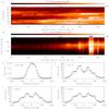 |
Fig. 1 Evolution of profiles of EE1 observed on Nov. 16 around 22:55. The profile of the Si iii line splits into two components; over several minutes upflow and downflow stay unchanged within the 0.3′′ wide slit. |
On Nov. 16, 2010, SUMER observed the leading sunspot of active region 11124. The slit of size 0.3′′ × 120′′ was placed in a way that during one hour the drift by the solar rotation would allow us to image the entire spot. A spectral window around the optically thin emission line of Si iii at 12.06 nm was read out at a cadence of 10 s. Standard data reduction procedures were applied to process the data set. In Fig. 1 we show the drift scan as y − t plot (top), the λ − t plot (below top) and line profiles in pixel 42 as indicated by the dashed line. At this location in the plage area very close to the sunspot, a rapid brightness increase by a factor of ≥ 20 is observed at time step 91. The pre-event profiles have been averaged and three more profiles are shown at different times during the event. The timing is indicated by blue arrows. Interestingly, the spectral line seems to split into two main components that are symmetrically shifted by 40 km s-1 towards the red and towards the blue with additional components at ± 100 km s-1 that are less strong. The lightcurve is not flat, it has two maxima that are separated by ≈ 120 s, but the overall shape with four peaks does not change over more than three minutes.
A similar observation with EE2 was completed on Nov. 19, 2010, when the instrument was pointed to the leading sunspot in AR 11126. Again, a stationary double-component EE with velocities of ± 35 km s-1 is observed from 21:53:14 to 21:57:14 in a plage location. Similar to the case of EE1, the brightness jumps by a factor of 10 and the lightcurve is double-peaked (cf., Fig. 2). During both events the Sun has rotated by ≈ 0.4′′, which is significantly below the spatial resolution of SUMER of 1.5′′.
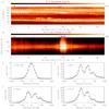 |
Fig. 2 Evolution of profiles of EE2 observed on Nov. 19 around 21:55. Again, the line profile splits quasi-stationary into two components. |
As a by-product of this study we identified two emission lines that were also recorded in the Si iii window and are not included in the SUMER spectral atlas (Curdt et al. 2001) as S i lines. In the atlas the Si iii window was recorded on the bare photocathode, while in this data set we could place it on the KBr-coated photocathode. All S i lines at 120.204 nm, 120.261 nm, 120.344 nm, 120.435 nm,120.559 nm, 120.613 nm, 120.704 nm, 120.776 nm, 120.886 nm, 121.122 nm, and 121.018 nm are present in SUMER spectra.
3. Discussion
In both events discussed here the Doppler-flow indicates symmetrical flows of ≈ 40 km s-1. It is unclear whether the 100 km s-1 components of EE1 are Doppler flows, because they can also be interpreted as blends by the S i lines at 120.613 nm and 120.704 nm (as discussed above). If they were interpreted as Doppler flow, this would imply a multi-component event with two sources in the slit area. Because of the ambiguity however, we do not discuss this question any further.
The Doppler-flow pattern seen in the line profiles is almost unchanged in magnitude of the line shift and in the location along the slit. This excludes any lateral movement exceeding ≈ 500 km along or across the slit within the 3-min duration of the event. Within 3 min however, a bidirectional jet moving at 40 km s-1 should have reached 7200 km in each component. This requires the direction of the jet to deviate less than 1° from the LOS. This scenario is very unlikely. It is simply not possible that in such an event upflow and downflow stay stationary over minutes within the 0.3′′ wide slit. Also the fact, that no increase in size along the slit is observed is a strong argument against a linear moving, collimated jet. A similar argument holds for EE2, which lasts even longer.
The conflict of lacking apparent motion is so evident in the examples shown here that we now adopt the alternative flow configuration. If we assume a spicule-like feature that is as narrow as the spectrometer slit and crosses the slit at some angle below 90°, then the redshifted portion and the blueshifted portion will appear simultaneously in spectroscopic data and can stay without apparent motion for an extended period of time, exactly as observed in EE1 and in EE2.
The double peak in the emission of EE1 and EE2 may also be an effect of the spinning motion if we assume the repetition of a brightness maximum after completing a full revolution after ≈ 200 s. Alternatively, the double-peaked lightcurve may have something to do with the occurrence of double-threaded jets that have been reported from XRT observations (Kamio et al. 2010).
Motivated by the plausible solution of the old discrepancy, we looked for suitable candidates of solar phenomena as conceivable counterparts for our double-component EEs. These candidates could be type II spicules or rapid blueshifted events (RBEs; De Pontieu et al. 2009, 2011; McIntosh et al. 2009; Rouppe van der Voort 2009) because they have very similar characteristics in terms of velocity, lifetime, size, and repeatability. A direct proof of helicity in RBEs through imaging instruments has to our knowledge not been reported yet and may be difficult to achieve. There is, however, indirect evidence, because rotation in macrospicules – believed to be bundles of substructures – was often observed. And focusing on smaller structures, evidence for helicity in regular spicules has been reported in literature, as already mentioned. Figure 3 shows several spicules and a macrospicule in a SUMER raster in O v obtained on August 18, 1996, in a coronal hole location. The panels show a brightness raster (left) and a dopplergram (right). Obviously, the macrospicule is spinning like a bent cylinder, but there is no signature of this motion in the spectroheliogram. This demonstrates that even in these large structures imagers are principally unable to observe the rotation unless finestructures can be resolved. Similar observations of “tornados” have been reported by Pike & Mason (1998) from SoHO-CDS data. We use the observed helicity in a macrospicule – a much more extended feature than the EEs discussed here – together with the published premise of no obvious distinction between macrospicules and other spicules as support for our argument.
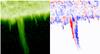 |
Fig. 3 Macrospicule at the solar limb near the south pole is observed in the light of the O v line at 62.9 nm, corresponding to 230 000 K; pseudo colours represent radiance (left) and Doppler motion (right). The Doppler flows are scaled from +30 km s-1 (red) to –30 km s-1 (blue). One half of the plasma ejection moves towards us, the other half away from us; the spicule swirls like a tornado along a magnetic field line with an Earth-sized diameter rotating at ± 30 km s-1. |
The cartoon in Fig. 4 shows typical SUMER line profiles calculated for a spiraling spicule at various aspect angles. We assume three components of the total radiance, two of which are taken from the spinning motion with a tangential velocity of ± 60 km s-1 that contribute with 47.5% each. As the third component we assume a faint flow of 100 km s-1 along the spicule – typical for type-II spicules – that contributes with 5%. The angle between spicule (or upflow) and LOS, θ, is set as 0°, 30°, 45°, 90°, 135°, 150°, and 180° for the seven cases (the cases with θ > 90° are mirror symmetric to cases (A) to (C) and not shown in Fig. 4). The spectrum in case (C) is very similar to those presented here and can quantitatively reproduce our observations.
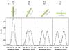 |
Fig. 4 Cartoon showing the suggested configuration; blue arrows indicate the spin, violet arrows the flow direction. We assume three-component emission, red and blue components from the spinning spicules (dot-dashed, each accounting for 47.5% of the total emission), the third component is the faint upflow along spicules (dashed lines, 5% of the total emission). The Gaussian width of each component is set to a typical value of 35 km s-1. The spectral resolution is 11 km s-1, comparable to a SUMER pixel. The composed emission is shown as the diamonds connected by solid lines. |
In many observations the red and the blue component of the EE are observed together with a component at rest. We attribute this zero-velocity component to the background emission of the solar disk that is also visible in optical thin emission. In our case, however, the foreground emission of the EEs is so much stronger that it outshines the background.
That in SUMER spectra no EEs are observed in coronal lines – besides the fact that no really good coronal lines for disk observations exist in the SUMER wavelength range – does not contradict the scenario suggested by De Pontieu et al. (2011), who found that the heated volume is outside the leading edge of the jet. If heating takes place while the jet propagates and expands, then spectrometers, in particular slow spectrometers, will have difficulties to observe this heating process.
Although none of the AIA channels covers the temperature regime around 46 000 K, the formation temperature of Si iii, we tried to find out whether signatures of the SUMER EEs are found in SDO-AIA images, but without success. This is plausible for a feature that is as narrow as the size of the SUMER slit and – in contrast to the macrospicule shown in Fig. 3 – below the AIA spatial resolution of 1.2′′.
The radius of the macrospicule in Fig. 3, r, is measured to be 5500 km. At the periphery, the Doppler flow is v = ± 30 km s-1. This allows us to determine the centripetal acceleration ac = v2/r. The value ac = 0.18 km s-2 is comparable to the gravitational acceleration. Pasachoff et al. (1968) performed a similar exercise for spinning spicules and arrived at a value of ac = 1.8 km s-2. From the examples shown as EE1 and EE2, which are much smaller than the macrospicule, we estimate a value of ac = 7 km s-2 assuming v = ± 40 km s-1 and r as about the slit size of 0.3′′. Similar values can be expected if we adopt the typical parameters mentioned by Teriaca et al. (2004), namely a diameter of 2′′ and a velocity of 150 km s-1. These violent motions could contribute to the solar wind acceleration (Pasachoff et al. 1968).
4. Conclusion
We propose that disk EEs and limb spicules are the same phenomenon. However, we assume an alternative configuration to explain the flows. Clearly, helicity is behind both manifestations and should be included to understand the physical nature of EEs. The assumption of a swirling narrow cylindrical body, rotating while upflowing, can reproduce observations by imagers as well as spectroscopes, which can explain the discrepancy between spectroscopic motion and apparent motion. Also, the statistical blueshift dominance of EEs would be an obvious consequence in this scenario (see Fig. 4, case c). Although our observations do not strictly exclude the possibility of bidirectional jets, there are good reasons to assume that EEs are indeed the spectroscopic signature of spinning type II spicules crossing the spectrometer slit in many cases. Even more, there seems to be no obvious distinction between macrospicules and microspicules or between blinkers and EEs.
The swirling component is normally not detectable by filtergraph instruments, but adds considerably to the energy released
by the apparent motion that is detected by these instruments. We note that the scenario of spinning spicule-like features that are rooted in the photosphere requires photospheric or even subsurface sources, which is not compatible with the model of reconnection events in the TR. This aspect may require the distinction of different types of EEs and calls for more systematic work. We speculate that the helicity may be related to global helicity as generated by the differential rotation. Alternatively, local reconnection caused by the subsurface turbulence in twisted flux tubes as discussed in MHD models could be a possible driving mechanism. In this context, it would be worthwhile to study the chirality of the events and look for different preferences in both hemispheres. These hypotheses are, however, not supported by our data and beyond the scope of this communication.
The IRIS mission – providing fast spectroscopic capabilities complemented by a chromospheric imager – will be an ideal platform for systematic statistical analyses of geometrical effects and their imprints on the centre-to-limb variation of red-blue tilt, red-blue asymmetry, birth rate, and mean velocity of EEs and also assessing the dominance of helicity in EEs in a quantitative manner.
Acknowledgments
The SUMER project is financially supported by DLR, CNES, NASA, and the ESA PRODEX Programme. SUMER is part of SoHO of ESA and NASA. H.T. is supported by the ASP Postdoctoral Fellowship Program of NCAR. The National Center for Atmospheric Research is sponsored by the National Science Foundation. We thank I. E. Dammasch, who spotted the beautiful macrospicule for the SUMER image galleries. We also thank B. N. Dwivedi for critical comments that helped to improve the clarity of this communication.
References
- Beckers, J. M. 1972, ARA&A, 10, 73 [NASA ADS] [CrossRef] [Google Scholar]
- Carlqvist, P. 1979, Sol. Phys., 63, 353 [NASA ADS] [CrossRef] [Google Scholar]
- Curdt, W., Brekke, P., Feldman, U., et al. 2001, A&A, 375, 591 [NASA ADS] [CrossRef] [EDP Sciences] [Google Scholar]
- De Pontieu, B., McIntosh, S. W., Carlsson, M., et al. 2009, ApJ, 701, L1 [NASA ADS] [CrossRef] [Google Scholar]
- De Pontieu, B., McIntosh, S. W., Carlsson, M., et al. 2011, Science, 331, 55 [NASA ADS] [CrossRef] [Google Scholar]
- Dere, K. P., Bartoe, J.-D. F., & Brueckner, G. E. 1984, ApJ 281, 870 [Google Scholar]
- Dere, K. P., Bartoe, J.-D. F., & Brueckner, G. E. 1989, Sol. Phys., 123, 41 [NASA ADS] [CrossRef] [Google Scholar]
- Innes, D. E. 2001, in transition region: Explosive Events, Encyclopedia of Astronomy and Astrophysics, ed. P. Murdin (Bristol: IOP Publ.) [Google Scholar]
- Innes, D. E. 2004, in Proc. SoHO 13: A Joint View from SoHO and TRACE, ed. H. Lacoste, Palma de Mallorca Oct. 2003, ESA SP, 547, 215 [Google Scholar]
- Innes, D. E., & Tóth, G. 1999, Sol. Phys., 185, 127 [NASA ADS] [CrossRef] [Google Scholar]
- Innes, D. E., Inhester, B., Axford, W. I., & Wilhelm, K. 1997, Nature, 386, 811 [NASA ADS] [CrossRef] [Google Scholar]
- Kamio, S., Curdt, W., Teriaca, L., et al. 2010, A&A, 510, L1 [NASA ADS] [CrossRef] [EDP Sciences] [Google Scholar]
- Liu, C., Deng, N., Liu, R., et al. 2011, ApJ, 735, L18 [NASA ADS] [CrossRef] [Google Scholar]
- Madjarska, M. S., & Doyle, J. G. 2002, A&A, 382, 319 [NASA ADS] [CrossRef] [EDP Sciences] [Google Scholar]
- Madjarska, M. S., & Doyle, J. G. 2003, A&A, 403, 731 [NASA ADS] [CrossRef] [EDP Sciences] [Google Scholar]
- Madjarska, M. S., Doyle, J. G., Hochedez, J.-F., et al. 2006, A&A, 452, L11 [NASA ADS] [CrossRef] [EDP Sciences] [Google Scholar]
- Madjarska, M. S., Doyle, J. G., & de Pontieu, B. 2009, ApJ, 701, 253 [CrossRef] [Google Scholar]
- McIntosh, S. W., & De Pontieu, B. 2009, ApJ, 707, 524 [NASA ADS] [CrossRef] [Google Scholar]
- Ning, Z., Innes, D. E., & Solanki, S. K. 2004, A&A, 419, 1141 [NASA ADS] [CrossRef] [EDP Sciences] [Google Scholar]
- Nisticó, G., Bothmer, V., Patsourakos, S., et al. 2009, Sol. Phys. 259, 87 [Google Scholar]
- Pasachoff, J. M., Noyes, R. W., & Beckers, J. M. 1968, Sol. Phys., 5, 131 [NASA ADS] [CrossRef] [Google Scholar]
- Pike, C. D., & Mason, H. E. 1998, Sol. Phys., 182, 333 [NASA ADS] [CrossRef] [Google Scholar]
- Shen, Y., Liu, Y., Su, J., & Ibrahim, A. 2011, ApJ, 735, L43 [NASA ADS] [CrossRef] [Google Scholar]
- Sterling, A. C., Harra, L. K., & Moore, R. L. 2010, ApJ, 722, 1644 [NASA ADS] [CrossRef] [Google Scholar]
- Teriaca, L., Banerjee, D., Falchi, A., et al. 2004, A&A, 427, 1065 [NASA ADS] [CrossRef] [EDP Sciences] [Google Scholar]
- Tian, H., Curdt, W., Marsch, E., & He, J.-S. 2008, ApJ, 681, L121 [Google Scholar]
- Rouppe van der Voort, L., Leenaarts, J., De Pontieu, B., et al. 2009, ApJ, 705, 272 [NASA ADS] [CrossRef] [Google Scholar]
- Wilhelm, K. 2000, A&A, 360, 351 [NASA ADS] [Google Scholar]
- Wilhelm, K., Curdt, W., Marsch, E., et al. 1995, Sol. Phys., 162, 189 [NASA ADS] [CrossRef] [Google Scholar]
- Zhang, M., Xia, L.-D., Tian, H., & Chen, Y. 2010, A&A, 520, A37 [NASA ADS] [CrossRef] [EDP Sciences] [Google Scholar]
All Figures
|
Fig. 1 Evolution of profiles of EE1 observed on Nov. 16 around 22:55. The profile of the Si iii line splits into two components; over several minutes upflow and downflow stay unchanged within the 0.3′′ wide slit. |
| In the text | |
|
Fig. 2 Evolution of profiles of EE2 observed on Nov. 19 around 21:55. Again, the line profile splits quasi-stationary into two components. |
| In the text | |
|
Fig. 3 Macrospicule at the solar limb near the south pole is observed in the light of the O v line at 62.9 nm, corresponding to 230 000 K; pseudo colours represent radiance (left) and Doppler motion (right). The Doppler flows are scaled from +30 km s-1 (red) to –30 km s-1 (blue). One half of the plasma ejection moves towards us, the other half away from us; the spicule swirls like a tornado along a magnetic field line with an Earth-sized diameter rotating at ± 30 km s-1. |
| In the text | |
|
Fig. 4 Cartoon showing the suggested configuration; blue arrows indicate the spin, violet arrows the flow direction. We assume three-component emission, red and blue components from the spinning spicules (dot-dashed, each accounting for 47.5% of the total emission), the third component is the faint upflow along spicules (dashed lines, 5% of the total emission). The Gaussian width of each component is set to a typical value of 35 km s-1. The spectral resolution is 11 km s-1, comparable to a SUMER pixel. The composed emission is shown as the diamonds connected by solid lines. |
| In the text | |
Current usage metrics show cumulative count of Article Views (full-text article views including HTML views, PDF and ePub downloads, according to the available data) and Abstracts Views on Vision4Press platform.
Data correspond to usage on the plateform after 2015. The current usage metrics is available 48-96 hours after online publication and is updated daily on week days.
Initial download of the metrics may take a while.