© ESO, 2011

1. Introduction

It is now well established that the Hanle effect serves as a diagnostic tool to determine the deterministic or turbulent weak magnetic fields on the Sun (see e.g., Stenflo 1982; Trujillo Bueno et al. 2004). The Hanle effect is a magnetic modification of the Rayleigh scattering spectral line polarization. The scattering polarization signatures in strong resonance lines are particularly sensitive to the frequency redistribution mechanism used in their computation. In the case of Rayleigh scattering, the differences in Q/I computed using angle-averaged and angle-dependent partial frequency redistribution (PRD) functions is between 10% and 30% (Sampoorna et al. 2011, see also Faurobert 1988). In the presence of weak magnetic fields, Nagendra et al. (2002) showed that the Stokes U is very sensitive to the angle-averaging of the redistribution function. However, these authors used a computationally expensive numerical method to solve the polarized line transfer equation including angle-dependent PRD function and the Hanle effect. Our aim here is to present an approximate method based on the concept of the single scattering approximation (see Frisch et al. 2009; Frisch 2010; Anusha et al. 2010; Sampoorna et al. 2011) to solve the above-mentioned problem efficiently.

The problem of angle-dependent PRD is characterized by intricate coupling between angle and frequency variables. This makes the evaluation of scattering integrals, and the solution of polarized transfer equation a challenging problem. A decomposition technique to reduce the non-axisymmetric Stokes transfer equation to cylindrically symmetric one was developed by Frisch (2007), for the case of an angle-averaged PRD with the Hanle effect. This technique was extended by Frisch (2009) to handle angle-dependent PRD with the Hanle effect. Basically the Stokes vector (I,Q,U) is first decomposed into a set of six irreducible components ${\mathit{I}}_{\mathit{Q}}^{\mathit{K}}$. In the particular case of angle-dependent PRD, these components are also non-axisymmetric. An azimuthal Fourier expansion of the angle-dependent PRD

functions then allows us to further reduce ${\mathit{I}}_{\mathit{Q}}^{\mathit{K}}$ into an infinite set of cylindrically symmetric Fourier coefficients $\stackrel{}{{{\mathit{I}}_{\mathit{Q}}^{\mathrm{\left(}\mathit{k}\mathrm{\right)}\mathit{K}}}_{\mathrm{˜}}}$. This method helps us to construct an infinite set of integral equations for the Fourier coefficients of the irreducible source vector components. As shown in Frisch (2010), the problem simplifies when the magnetic field is set to zero or assumed to be turbulent. In this case, the Fourier wavenumber k takes only the values k = 0,1,2, and four components $\stackrel{}{{{\mathit{I}}_{\mathit{Q}}^{\mathrm{\left(}\mathit{k}\mathrm{\right)}\mathit{K}}}_{\mathrm{˜}}}$ are sufficient to represent the polarized radiation field. As shown in Sampoorna et al. (2011), the polarized radiation field can be calculated by solving a set of integral equations for the corresponding cylindrically symmetric irreducible source vector components. Several numerical methods are described in this reference : two accelerated lambda iteration (ALI) methods, associated with either a core-wing or a frequency-angle by frequency-angle technique, and one scattering expansion method, based on a Neumann series expansion in terms of the mean number of scattering events.

For the Hanle effect with an angle-dependent PRD, the numerical solution is possible only if one truncates the infinite set of integral equations for the Fourier coefficients of the irreducible source vector components. For the type II PRD function (frequency coherent scattering in the atomic rest frame) of Hummer (1962), Domke & Hubeny (1988) showed that, at least five terms in the azimuthal Fourier expansion are needed to get a good agreement with the exact value of the function. This implies that the azimuthal order k takes values 0,  ± 1,  ± 2,  ± 3, and  ± 4, for each combination of K and Q of the irreducible source vector. For the Hanle problem, K = 0 and 2, with  − K ≤ Q ≤  + K. Hence, we obtain a total of 54 coupled integral equations. Although they can be numerically solved, it is computationally demanding. To simplify this numerically difficult problem, we present an approximate method of solution based on the concept of a single scattering approximation.

In Sect. 2, we briefly recall the decomposition technique presented in Frisch (2009) for the Hanle effect with angle-dependent PRD. In Sect. 3, we derive approximate expressions for the Fourier coefficients of irreducible source vector components applying the single scattering approximation. A generic form for the Hanle scattering redistribution matrix is assumed in Sects. 2 and 3 (see Eq. (4) below). In Sect. 4, we generalize the results of Sects. 2 and 3 to the Hanle scattering redistribution matrix derived by Bommier (1997b, the so-called approximation-II). Section 5 is devoted to the comparison of results computed using the single scattering approximation with those computed using the perturbation method of Nagendra et al. (2002). Conclusions are presented in Sect. 6. Some technical details are given in Appendices A and B.

2. A decomposition method for Hanle effect with angle-dependent PRD

For the sake of clarity, we recall some important equations from Frisch (2009). The polarized transfer equation for the Stokes vector can be written in component form as $\mathit{\mu }\frac{\mathit{\partial }{\mathit{I}}_{\mathit{i}}}{\mathit{\partial \tau }}\mathrm{=}\left[\mathit{\varphi }\mathrm{\left(}\mathit{x}\mathrm{\right)}\mathrm{+}\mathit{r}\right]\left[{\mathit{I}}_{\mathit{i}}\mathrm{\left(}\mathit{\tau ,x,}\mathbf{\Omega }\mathrm{\right)}\mathrm{-}{\mathit{S}}_{\mathit{i}}\mathrm{\left(}\mathit{\tau ,x,}\mathbf{\Omega }\mathrm{\right)}\right]\mathit{,}\mathit{i}\mathrm{=}\mathrm{0}\mathit{,}\mathrm{1}\mathit{,}\mathrm{2}\mathit{,}$(1)where Ω  (θ,χ) is the outgoing ray direction defined with respect to the atmospheric normal and μ = cosθ. The line optical depth τ is defined by    dτ =  −k_l   dz, where k_l is the frequency–averaged line absorption coefficient, and ϕ(x) is the normalized Voigt function. The frequency x is measured in units of the Doppler width, with x = 0 at the line center. The ratio of continuum to line absorption coefficient is denoted by r. The total source vector is given by ${\mathit{S}}_{\mathit{i}}\mathrm{\left(}\mathit{\tau ,x,}\mathbf{\Omega }\mathrm{\right)}\mathrm{=}\frac{\mathit{\varphi }\mathrm{\left(}\mathit{x}\mathrm{\right)}{\mathit{S}}_{\mathit{l,i}}\mathrm{\left(}\mathit{\tau ,x,}\mathbf{\Omega }\mathrm{\right)}\mathrm{+}\mathit{r}{\mathit{S}}_{\mathit{c,i}}}{\mathit{\varphi }\mathrm{\left(}\mathit{x}\mathrm{\right)}\mathrm{+}\mathit{r}}\mathit{,}$(2)where S_c,i are the components of the unpolarized continuum source vector. We assume that S_c,0 = B_ν0, where B_ν0 is the Planck function at the line center, and S_c,1 = S_c,2 = 0. The line source vector can be written as $\begin{array}{ccc}& & {\mathit{S}}_{\mathit{l,i}}\mathrm{\left(}\mathit{\tau ,x,}\mathbf{\Omega }\mathrm{\right)}\mathrm{=}{\mathit{G}}_{\mathit{i}}\mathrm{\left(}\mathit{\tau }\mathrm{\right)}\\ & & \mathrm{+}\mathrm{\int }\mathrm{􏽉}\sum _{\mathit{j}\mathrm{=}\mathrm{0}}^{\mathrm{2}}\frac{{\mathit{R}}_{\mathit{ij}}\mathrm{\left(}\mathit{x,}\mathbf{\Omega }\mathit{,}{\mathit{x}}^{\mathrm{\prime }}\mathit{,}{\mathbf{\Omega }}^{\mathrm{\prime }}\mathit{,}{B}\mathrm{\right)}}{\mathit{\varphi }\mathrm{\left(}\mathit{x}\mathrm{\right)}}{\mathit{I}}_{\mathit{j}}\mathrm{\left(}\mathit{\tau ,}{\mathit{x}}^{\mathrm{\prime }}\mathit{,}{\mathbf{\Omega }}^{\mathrm{\prime }}\mathrm{\right)}\frac{\hspace{0.17em}\mathrm{d}{\mathrm{\Omega }}^{\mathrm{\prime }}}{\mathrm{4}\mathit{\pi }}\hspace{0.17em}\mathrm{d}{\mathit{x}}^{\mathrm{\prime }}\mathit{,}\end{array}$(3)where Ω′  (θ′,χ′) is the direction of the incoming ray defined with respect to the atmospheric normal, and    dΩ′ = sinθ′   dθ′   dχ′. For simplicity, we assume that the primary source is unpolarized, namely that only G₀(τ) is non-zero, and it is proportional to B_ν0. In Sect. 3, we assume a generic form for the elements of the redistribution matrix in the presence of a weak magnetic field B given by ${\mathit{R}}_{\mathit{ij}}\mathrm{\left(}\mathit{x,}\mathbf{\Omega }\mathit{,}{\mathit{x}}^{\mathrm{\prime }}\mathit{,}{\mathbf{\Omega }}^{\mathrm{\prime }}\mathit{,}{B}\mathrm{\right)}\mathrm{=}\mathit{r}\mathrm{\left(}\mathit{x,}{\mathit{x}}^{\mathrm{\prime }}\mathit{,}\mathrm{\Theta }\mathrm{\right)}{\mathit{P}}_{\mathit{ij}}\mathrm{\left(}\mathbf{\Omega }\mathit{,}{\mathbf{\Omega }}^{\mathrm{\prime }}\mathit{,}{B}\mathrm{\right)}\mathit{,}$(4)where r(x,x′,Θ) is any redistribution function with proper normalization conditions, such as the type I, II, or III PRD functions of Hummer (1962), and Θ is the angle between the incoming (Ω′) and outgoing (Ω) rays. In terms of the irreducible spherical tensors ${\mathrm{𝒯}}_{\mathit{Q}}^{\mathit{K}}\mathrm{\left(}\mathit{i,}\mathbf{\Omega }\mathrm{\right)}$ introduced by Landi Degl’Innocenti (1984), the Hanle phase matrix elements can be written as (see Chaps. 5 and 10 of Landi Degl’Innocenti & Landolfi 2004; or Frisch 2007; 2009) $\begin{array}{ccc}& & {\mathit{P}}_{\mathit{ij}}\mathrm{\left(}\mathbf{\Omega }\mathit{,}{\mathbf{\Omega }}^{\mathrm{\prime }}\mathit{,}{B}\mathrm{\right)}\\ & \mathrm{=}& \sum _{\mathit{KQ}}{\mathrm{𝒯}}_{\mathit{Q}}^{\mathit{K}}\mathrm{\left(}\mathit{i,}\mathbf{\Omega }\mathrm{\right)}\sum _{{\mathit{Q}}^{\mathrm{\prime }}}{\mathrm{𝒩}}_{\mathit{Q}{\mathit{Q}}^{\mathrm{\prime }}}^{\mathit{K}}\mathrm{\left(}{B}\mathrm{\right)}\mathrm{(}\mathrm{-}\mathrm{1}{\mathrm{)}}^{{\mathit{Q}}^{\mathrm{\prime }}}{\mathrm{𝒯}}_{\mathrm{-}{\mathit{Q}}^{\mathrm{\prime }}}^{\mathit{K}}\mathrm{(}\mathit{j,}{\mathbf{\Omega }}^{\mathrm{\prime }}\mathrm{)}\mathit{.}\end{array}$(5)For the coefficients ${\mathrm{𝒩}}_{\mathit{Q}{\mathit{Q}}^{\mathrm{\prime }}}^{\mathit{K}}$ we assume the simple form ${\mathrm{𝒩}}_{\mathit{Q}{\mathit{Q}}^{\mathrm{\prime }}}^{\mathit{K}}\mathrm{\left(}{B}\mathrm{\right)}\mathrm{=}\mathrm{(}\mathrm{1}\mathrm{-}\mathit{ϵ}\mathrm{)}{\mathit{W}}_{\mathit{K}}{\mathrm{ℳ}}_{\mathit{Q}{\mathit{Q}}^{\mathrm{\prime }}}^{\mathit{K}}\mathrm{\left(}{\mathit{\theta }}_{\mathit{B}}\mathit{,}{\mathit{\chi }}_{\mathit{B}}\mathit{,}\mathrm{\Gamma }\mathrm{\right)}\mathit{,}$(6)where ${\mathrm{ℳ}}_{\mathit{Q}{\mathit{Q}}^{\mathrm{\prime }}}^{\mathit{K}}$ are coefficients that describe the effects of the magnetic field, ϵ the thermalization parameter, W_K the depolarizability factors depending on the J-quantum numbers of upper and lower levels, (θ_B,χ_B) the polar angles defining the magnetic field orientation with respect to the atmospheric normal, and Γ = 2πν_Lg_u/A_ul in standard notation is the Hanle parameter.

The Stokes vector and the source vector can each be decomposed into six irreducible components ${\mathit{I}}_{\mathit{Q}}^{\mathit{K}}$ and ${\mathit{S}}_{\mathit{Q}}^{\mathit{K}}$ that are non-axisymmetric because of the angle dependence of the PRD function. To describe this angle dependence of the PRD function, we introduce an azimuthal Fourier expansion written as (see Eq. (15) of Frisch 2009) $\mathit{r}\mathrm{\left(}\mathit{x,}{\mathit{x}}^{\mathrm{\prime }}\mathit{,}\mathrm{\Theta }\mathrm{\right)}\mathrm{=}\frac{\mathrm{1}}{\mathrm{2}}\sum _{\mathit{k}\mathrm{=}\mathrm{-}\mathrm{\infty }}^{\mathit{k}\mathrm{=}\mathrm{+}\mathrm{\infty }}\stackrel{}{{{\mathit{r}}^{\mathrm{\left(}\mathit{k}\mathrm{\right)}}}_{\mathrm{˜}}}\mathrm{\left(}\mathit{x,\theta ,}{\mathit{x}}^{\mathrm{\prime }}\mathit{,}{\mathit{\theta }}^{\mathrm{\prime }}\mathrm{\right)}{\mathrm{e}}^{\mathrm{i}\mathit{k}\mathrm{(}\mathit{\chi }\mathrm{-}{\mathit{\chi }}^{\mathrm{\prime }}\mathrm{)}}\mathit{,}$(7)where $\begin{array}{ccc}& & \stackrel{}{{{\mathit{r}}^{\mathrm{\left(}\mathit{k}\mathrm{\right)}}}_{\mathrm{˜}}}\mathrm{\left(}\mathit{x,\theta ,}{\mathit{x}}^{\mathrm{\prime }}\mathit{,}{\mathit{\theta }}^{\mathrm{\prime }}\mathrm{\right)}\mathrm{=}\mathrm{(}\mathrm{1}\mathrm{+}{\mathit{\delta }}_{\mathrm{0}\mathit{k}}\mathrm{)}\frac{\mathrm{2}\mathrm{-}{\mathit{\delta }}_{\mathrm{0}\mathit{k}}}{\mathrm{2}\mathit{\pi }}\\ & & \mathrm{\times }{\mathrm{\int }}_{\mathrm{0}}^{\mathrm{2}\mathit{\pi }}\mathit{r}\mathrm{(}\mathit{x,\theta ,}{\mathit{x}}^{\mathrm{\prime }}\mathit{,}{\mathit{\theta }}^{\mathrm{\prime }}\mathit{,\chi }\mathrm{-}{\mathit{\chi }}^{\mathrm{\prime }}\mathrm{)}\cos \mathrm{\left[}\mathit{k}\mathrm{\right(}\mathit{\chi }\mathrm{-}{\mathit{\chi }}^{\mathrm{\prime }}\mathrm{\left)}\mathrm{\right]}\hspace{0.17em}\mathrm{d}\mathrm{(}\mathit{\chi }\mathrm{-}{\mathit{\chi }}^{\mathrm{\prime }}\mathrm{)}\mathit{.}\end{array}$(8)It is easy to verify that $\stackrel{}{{{\mathit{r}}^{\mathrm{\left(}\mathit{k}\mathrm{\right)}}}_{\mathrm{˜}}}\mathrm{=}\stackrel{}{{{\mathit{r}}^{\mathrm{(}\mathrm{-}\mathit{k}\mathrm{)}}}_{\mathrm{˜}}}$. To describe the azimuthal dependence of the irreducible components ${\mathit{I}}_{\mathit{Q}}^{\mathit{K}}$, we introduce the Fourier decomposition ${\mathit{I}}_{\mathit{Q}}^{\mathit{K}}\mathrm{\left(}\mathit{\tau ,x,}\mathbf{\Omega }\mathrm{\right)}\mathrm{=}\frac{\mathrm{1}}{\mathrm{2}}\sum _{\mathit{k}\mathrm{=}\mathrm{-}\mathrm{\infty }}^{\mathit{k}\mathrm{=}\mathrm{+}\mathrm{\infty }}\stackrel{}{{{\mathit{I}}_{\mathit{Q}}^{\mathrm{\left(}\mathit{k}\mathrm{\right)}\mathit{K}}}_{\mathrm{˜}}}\mathrm{\left(}\mathit{\tau ,x,\theta }\mathrm{\right)}{\mathrm{e}}^{\mathrm{i}\mathit{k\chi }}\mathit{.}$(9)Assuming a similar expansion for the primary source term ${\mathit{G}}_{\mathit{Q}}^{\mathit{K}}$, it is easy to show that ${\mathit{S}}_{\mathit{Q}}^{\mathit{K}}$ has an azimuthal expansion similar to Eq. (9).

The Fourier coefficients $\stackrel{}{{{\mathit{I}}_{\mathit{Q}}^{\mathrm{\left(}\mathit{k}\mathrm{\right)}\mathit{K}}}_{\mathrm{˜}}}$ satisfy a non-local thermodynamic equilibrium (hereafter non-LTE) transfer equation $\mathit{\mu }\frac{\mathit{\partial }\stackrel{}{{{\mathit{I}}_{\mathit{Q}}^{\mathrm{\left(}\mathit{k}\mathrm{\right)}\mathit{K}}}_{\mathrm{˜}}}}{\mathit{\partial \tau }}\mathrm{=}\left[\mathit{\varphi }\mathrm{\left(}\mathit{x}\mathrm{\right)}\mathrm{+}\mathit{r}\right]\mathrm{\left[}\stackrel{}{{{\mathit{I}}_{\mathit{Q}}^{\mathrm{\left(}\mathit{k}\mathrm{\right)}\mathit{K}}}_{\mathrm{˜}}}\mathrm{\right(}\mathit{\tau ,x,\theta }\mathrm{)}\mathrm{-}\stackrel{}{{{\mathit{S}}_{\mathit{Q}}^{\mathrm{\left(}\mathit{k}\mathrm{\right)}\mathit{K}}}_{\mathrm{˜}}}\mathrm{(}\mathit{\tau ,x,\theta }{\mathrm{\left)}}^{\mathrm{\right]}}\mathit{,}$(10)where the source term is given by Eq. (2) with $\stackrel{}{{{\mathit{S}}_{\mathit{l,Q}}^{\mathrm{\left(}\mathit{k}\mathrm{\right)}\mathit{K}}}_{\mathrm{˜}}}$ and $\stackrel{}{{{\mathit{S}}_{\mathit{c,Q}}^{\mathrm{\left(}\mathit{k}\mathrm{\right)}\mathit{K}}}_{\mathrm{˜}}}$ instead of S_l,i and S_c,i. Since the continuum is assumed to be unpolarized, $\stackrel{}{{{\mathit{S}}_{\mathit{c,Q}}^{\mathrm{\left(}\mathit{k}\mathrm{\right)}\mathit{K}}}_{\mathrm{˜}}}\mathrm{=}\mathrm{2}{\mathit{\delta }}_{\mathrm{0}\mathit{k}}{\mathit{\delta }}_{\mathrm{0}\mathit{K}}{\mathit{\delta }}_{\mathrm{0}\mathit{Q}}{\mathit{B}}_{{\mathit{\nu }}_{\mathrm{0}}}$. The Fourier coefficients of the line source vector are given by 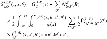$\begin{array}{ccc}& & \stackrel{}{{{\mathit{S}}_{\mathit{l,Q}}^{\mathrm{\left(}\mathit{k}\mathrm{\right)}\mathit{K}}}_{\mathrm{˜}}}\mathrm{\left(}\mathit{\tau ,x,\theta }\mathrm{\right)}\mathrm{=}\stackrel{}{{{\mathit{G}}_{\mathit{Q}}^{\mathrm{\left(}\mathit{k}\mathrm{\right)}\mathit{K}}}_{\mathrm{˜}}}\mathrm{\left(}\mathit{\tau }\mathrm{\right)}\mathrm{+}\sum _{{\mathit{Q}}^{\mathrm{\prime }}}{\mathrm{𝒩}}_{\mathit{Q}{\mathit{Q}}^{\mathrm{\prime }}}^{\mathit{K}}\mathrm{\left(}{B}\mathrm{\right)}\\ & & \mathrm{\times }\frac{\mathrm{1}}{\mathrm{2}}{\mathrm{\int }}_{\mathrm{-}\mathrm{\infty }}^{\mathrm{+}\mathrm{\infty }}{\mathrm{\int }}_{\mathrm{0}}^{\mathit{\pi }}\frac{\stackrel{}{{{\mathit{r}}^{\mathrm{\left(}\mathit{k}\mathrm{\right)}}}_{\mathrm{˜}}}\mathrm{\left(}\mathit{x,\theta ,}{\mathit{x}}^{\mathrm{\prime }}\mathit{,}{\mathit{\theta }}^{\mathrm{\prime }}\mathrm{\right)}}{\mathit{\varphi }\mathrm{\left(}\mathit{x}\mathrm{\right)}}\sum _{{\mathit{K}}^{\mathrm{\prime }}{\mathit{Q}}^{\mathrm{\prime \prime }}}\frac{\mathrm{1}}{\mathrm{2}}\stackrel{}{{{\mathrm{\Gamma }}_{\mathit{K}{\mathit{Q}}^{\mathrm{\prime }}\mathit{,}{\mathit{K}}^{\mathrm{\prime }}{\mathit{Q}}^{\mathrm{\prime \prime }}}^{\mathrm{(}\mathit{k}\mathrm{-}{\mathit{k}}^{\mathrm{\prime }}\mathrm{)}}}_{\mathrm{˜}}}\mathrm{\left(}{\mathit{\theta }}^{\mathrm{\prime }}\mathrm{\right)}\\ & & \mathrm{\times }\stackrel{}{{{\mathit{I}}_{{\mathit{Q}}^{\mathrm{\prime \prime }}}^{\mathrm{\left(}{\mathit{k}}^{\mathrm{\prime }}\mathrm{\right)}{\mathit{K}}^{\mathrm{\prime }}}}_{\mathrm{˜}}}\mathrm{\left(}\mathit{\tau ,}{\mathit{x}}^{\mathrm{\prime }}\mathit{,}{\mathit{\theta }}^{\mathrm{\prime }}\mathrm{\right)}\sin {\mathit{\theta }}^{\mathrm{\prime }}\hspace{0.17em}\mathrm{d}{\mathit{\theta }}^{\mathrm{\prime }}\hspace{0.17em}\mathrm{d}{\mathit{x}}^{\mathrm{\prime }}\mathit{,}\end{array}$(11)where the primary source term $\stackrel{}{{{\mathit{G}}_{\mathit{Q}}^{\mathrm{\left(}\mathit{k}\mathrm{\right)}\mathit{K}}}_{\mathrm{˜}}}\mathrm{\left(}\mathit{\tau }\mathrm{\right)}\mathrm{=}\mathrm{2}{\mathit{\delta }}_{\mathrm{0}\mathit{k}}{\mathit{\delta }}_{\mathrm{0}\mathit{K}}{\mathit{\delta }}_{\mathrm{0}\mathit{Q}}{\mathit{G}}_{\mathrm{0}}\mathrm{\left(}\mathit{\tau }\mathrm{\right)}$, and k′ = k + Q′ − Q′′. For a given value of k, the values of k′ are clearly restricted to k − 4 ≤ k′ ≤ k + 4. The non-zero azimuthal Fourier coefficients are of the form $\stackrel{}{{{\mathrm{\Gamma }}_{\mathit{K}{\mathit{Q}}^{\mathrm{\prime }}\mathit{,}{\mathit{K}}^{\mathrm{\prime }}{\mathit{Q}}^{\mathrm{\prime \prime }}}^{\mathrm{(}{\mathit{Q}}^{\mathrm{\prime \prime }}\mathrm{-}{\mathit{Q}}^{\mathrm{\prime }}\mathrm{)}}}_{\mathrm{˜}}}\mathrm{\left(}{\mathit{\theta }}^{\mathrm{\prime }}\mathrm{\right)}\mathrm{=}\sum _{\mathit{i}\mathrm{=}\mathrm{0}}^{\mathrm{2}}\mathrm{(}\mathrm{-}\mathrm{1}{\mathrm{)}}^{{\mathit{Q}}^{\mathrm{\prime }}}\stackrel{}{{{\mathrm{𝒯}}_{\mathrm{-}{\mathit{Q}}^{\mathrm{\prime }}}^{\mathit{K}}}_{\mathrm{˜}}}\mathrm{(}\mathit{i,}{\mathit{\theta }}^{\mathrm{\prime }}\mathrm{\left)}\stackrel{}{{{\mathrm{𝒯}}_{{\mathit{Q}}^{\mathrm{\prime \prime }}}^{{\mathit{K}}^{\mathrm{\prime }}}}_{\mathrm{˜}}}\mathrm{\right(}\mathit{i,}{\mathit{\theta }}^{\mathrm{\prime }}\mathrm{)}\mathit{,}$(12)where K and K′ are both even or both odd. The $\begin{array}{}{}_{\mathrm{˜}}\\ {\mathrm{𝒯}}_{\mathit{Q}}^{\mathit{K}}\end{array}\mathrm{\left(}\mathit{i,\theta }\mathrm{\right)}$ are combinations of trigonometric functions that may be written as ${\mathrm{𝒯}}_{\mathit{Q}}^{\mathit{K}}\mathrm{\left(}\mathit{i,}\mathbf{\Omega }\mathrm{\right)}\mathrm{=}\begin{array}{}{}_{\mathrm{˜}}\\ {\mathrm{𝒯}}_{\mathit{Q}}^{\mathit{K}}\end{array}\mathrm{\left(}\mathit{i,\theta }\mathrm{\right)}{\mathrm{e}}^{\mathrm{i}\mathit{Q\chi }}$. It is easy to verify that $\stackrel{}{{{\mathit{S}}_{\mathit{l,Q}}^{\mathrm{\left(}\mathit{k}\mathrm{\right)}\mathit{K}}}_{\mathrm{˜}}}$ satisfy the following conjugation property ${\mathrm{\left[}\stackrel{}{{{\mathit{S}}_{\mathit{l,Q}}^{\mathrm{\left(}\mathit{k}\mathrm{\right)}\mathit{K}}}_{\mathrm{˜}}}\mathrm{\right]}}^{\mathrm{\ast }}\mathrm{=}\mathrm{(}\mathrm{-}\mathrm{1}{\mathrm{)}}^{\mathit{Q}}\stackrel{}{{{\mathit{S}}_{\mathit{l,}\mathrm{-}\mathit{Q}}^{\mathrm{(}\mathrm{-}\mathit{k}\mathrm{)}\mathit{K}}}_{\mathrm{˜}}}\mathit{.}$(13)We note that the range of k values extends a priori from  − ∞ to  + ∞, thereby giving rise to an infinite set of integral equations for $\stackrel{}{{{\mathit{S}}_{\mathit{l,Q}}^{\mathrm{\left(}\mathit{k}\mathrm{\right)}\mathit{K}}}_{\mathrm{˜}}}\mathrm{\left(}\mathit{\tau ,x,\theta }\mathrm{\right)}$. A solution is possible only if we truncate this infinite set. As already noted in Sect. 1, if we restrict k to k = 0,    ± 1,    ± 2,    ± 3,    ± 4, we obtain a set of 54 coupled integral equations. Before going into such a difficult numerical problem, we show in the following section how the problem can be simplified by using a single scattering approximation (see Frisch et al. 2009; Frisch 2010).

3. Approximate expressions for the Fourier coefficients $\stackrel{}{{{\mathit{S}}_{{l}\mathit{,Q}}^{\mathrm{\left(}\mathit{k}\mathrm{\right)}\mathit{K}}}_{\mathrm{˜}}}\mathrm{\left(}\mathit{\tau ,x,\theta }\mathrm{\right)}$

First we make the reasonable assumption that Stokes I is unaffected by the polarization. We can thus describe Stokes I with ${\mathit{I}}_{\mathrm{0}}^{\mathrm{0}}$ only, neglecting the contributions of the K ≠ 0 terms. For an angle-dependent PRD, ${\mathit{I}}_{\mathrm{0}}^{\mathrm{0}}$ is non-axisymmetric and can be Fourier expanded as in Eq. (9). However, as Stokes I is almost independent of the magnetic field (in the weak field Hanle regime that we consider), we make a further assumption that ${\mathit{I}}_{\mathrm{0}}^{\mathrm{0}}$ is independent of χ. Hence, only the k = 0 term contributes to ${\mathit{I}}_{\mathrm{0}}^{\mathrm{0}}$ and we can write $\mathit{I}\mathrm{\simeq }{\mathit{I}}_{\mathrm{0}}^{\mathrm{0}}\mathrm{\simeq }\frac{\mathrm{1}}{\mathrm{2}}\stackrel{}{{{\mathit{I}}_{\mathrm{0}}^{\mathrm{\left(}\mathrm{0}\mathrm{\right)}\mathrm{0}}}_{\mathrm{˜}}}\mathit{.}$(14)With these approximations, the irreducible component ${\mathit{S}}_{\mathit{l,}\mathrm{0}}^{\mathrm{0}}$ takes a simple form, namely $\begin{array}{ccc}& & {\mathit{S}}_{\mathit{l,}\mathrm{0}}^{\mathrm{0}}\mathrm{\left(}\mathit{\tau ,x,\theta }\mathrm{\right)}\mathrm{\simeq }\mathit{ϵ}{\mathit{B}}_{{\mathit{\nu }}_{\mathrm{0}}}\mathrm{+}\mathrm{(}\mathrm{1}\mathrm{-}\mathit{ϵ}\mathrm{)}\\ & & \mathrm{\times }\frac{\mathrm{1}}{\mathrm{2}}{\mathrm{\int }}_{\mathrm{-}\mathrm{\infty }}^{\mathrm{+}\mathrm{\infty }}{\mathrm{\int }}_{\mathrm{0}}^{\mathit{\pi }}\frac{{\mathit{r}}^{\mathrm{\left(}\mathrm{0}\mathrm{\right)}}\mathrm{\left(}\mathit{x,\theta ,}{\mathit{x}}^{\mathrm{\prime }}\mathit{,}{\mathit{\theta }}^{\mathrm{\prime }}\mathrm{\right)}}{\mathit{\varphi }\mathrm{\left(}\mathit{x}\mathrm{\right)}}{\mathit{I}}_{\mathrm{0}}^{\mathrm{0}}\mathrm{\left(}\mathit{\tau ,}{\mathit{x}}^{\mathrm{\prime }}\mathit{,}{\mathit{\theta }}^{\mathrm{\prime }}\mathrm{\right)}\sin {\mathit{\theta }}^{\mathrm{\prime }}\hspace{0.17em}\mathrm{d}{\mathit{\theta }}^{\mathrm{\prime }}\hspace{0.17em}\mathrm{d}{\mathit{x}}^{\mathrm{\prime }}\mathit{,}\end{array}$(15)where ${\mathit{r}}^{\mathrm{\left(}\mathrm{0}\mathrm{\right)}}\mathrm{=}\stackrel{}{{{\mathit{r}}^{\mathrm{\left(}\mathrm{0}\mathrm{\right)}}}_{\mathrm{˜}}}\mathit{/}\mathrm{2}$, and the thermalization parameter ϵ = Γ_I/(Γ_R + Γ_I), with Γ_R and Γ_I being the radiative and inelastic collisional de-excitation rates.

To obtain approximate expressions for the Fourier components $\stackrel{}{{{\mathit{S}}_{\mathit{l,Q}}^{\mathrm{\left(}\mathit{k}\mathrm{\right)}\mathrm{2}}}_{\mathrm{˜}}}$ of ${\mathit{S}}_{\mathit{l,Q}}^{\mathrm{2}}$, we apply the single scattering approximation to Eq. (11), namely we keep in the right-hand side of this equation only the contribution from $\stackrel{}{{{\mathit{I}}_{\mathrm{0}}^{\mathrm{\left(}\mathrm{0}\mathrm{\right)}\mathrm{0}}}_{\mathrm{˜}}}$. This amounts to assuming that k′ = K′ = Q′′ = 0. Since k′ = k + Q′ − Q′′, we obtain k =  −Q′. Hence, only the components $\stackrel{}{{{\mathit{S}}_{\mathit{l,Q}}^{\mathrm{\left(}\mathit{k}\mathrm{\right)}\mathrm{2}}}_{\mathrm{˜}}}$ with k = 0, ± 1, ± 2 are non-zero. These 25 Fourier components are given by the following approximate expression $\begin{array}{ccc}& & \stackrel{}{{{\mathit{S}}_{\mathit{l,Q}}^{\mathrm{\left(}\mathit{k}\mathrm{\right)}\mathrm{2}}}_{\mathrm{˜}}}\mathrm{\left(}\mathit{\tau ,x,\theta }\mathrm{\right)}\mathrm{\simeq }{\mathrm{𝒩}}_{\mathit{Q}\mathrm{-}\mathit{k}}^{\mathrm{2}}\mathrm{\left(}{B}\mathrm{\right)}\frac{\mathrm{1}}{\mathrm{2}}{\mathrm{\int }}_{\mathrm{-}\mathrm{\infty }}^{\mathrm{+}\mathrm{\infty }}{\mathrm{\int }}_{\mathrm{0}}^{\mathit{\pi }}\frac{\stackrel{}{{{\mathit{r}}^{\mathrm{\left(}\mathit{k}\mathrm{\right)}}}_{\mathrm{˜}}}\mathrm{\left(}\mathit{x,\theta ,}{\mathit{x}}^{\mathrm{\prime }}\mathit{,}{\mathit{\theta }}^{\mathrm{\prime }}\mathrm{\right)}}{\mathit{\varphi }\mathrm{\left(}\mathit{x}\mathrm{\right)}}\\ & & \mathrm{\times }\stackrel{}{{{\mathrm{\Gamma }}_{\mathrm{2}\mathrm{-}\mathit{k,}\mathrm{00}}^{\mathrm{\left(}\mathit{k}\mathrm{\right)}}}_{\mathrm{˜}}}\mathrm{\left(}{\mathit{\theta }}^{\mathrm{\prime }}\mathrm{\right)}{\mathit{I}}_{\mathrm{0}}^{\mathrm{0}}\mathrm{\left(}\mathit{\tau ,}{\mathit{x}}^{\mathrm{\prime }}\mathit{,}{\mathit{\theta }}^{\mathrm{\prime }}\mathrm{\right)}\sin {\mathit{\theta }}^{\mathrm{\prime }}\hspace{0.17em}\mathrm{d}{\mathit{\theta }}^{\mathrm{\prime }}\hspace{0.17em}\mathrm{d}{\mathit{x}}^{\mathrm{\prime }}\mathit{.}\end{array}$(16)The explicit forms of the azimuthal Fourier coefficients $\stackrel{}{{{\mathrm{\Gamma }}_{\mathrm{2}\mathrm{-}\mathit{k,}\mathrm{00}}^{\mathrm{\left(}\mathit{k}\mathrm{\right)}}}_{\mathrm{˜}}}\mathrm{\left(}\mathit{\theta }\mathrm{\right)}$ are given in the Appendix A.

The irreducible components ${\mathit{S}}_{\mathit{l,Q}}^{\mathrm{2}}$ and their Fourier components for k ≠ 0 are complex numbers. We introduce here their real components. Following Frisch (2007, Eqs. (25) and (26)), we define the real components of ${\mathit{S}}_{\mathit{l,Q}}^{\mathrm{2}}$ to be ${\mathit{S}}_{\mathit{l,Q}}^{\mathrm{x}\mathrm{2}}\mathrm{=}\frac{\mathrm{1}}{\mathrm{2}}\mathrm{[}{\mathit{S}}_{\mathit{l,Q}}^{\mathrm{2}}\mathrm{+}\mathrm{(}\mathrm{-}\mathrm{1}{\mathrm{)}}^{\mathit{Q}}{{\mathit{S}}_{\mathit{l,}\mathrm{-}\mathit{Q}}^{\mathrm{2}}}^{\mathrm{]}}\mathit{,}$(17)${\mathit{S}}_{\mathit{l,Q}}^{\mathrm{y}\mathrm{2}}\mathrm{=}\mathrm{-}\frac{\mathrm{i}}{\mathrm{2}}\mathrm{[}{\mathit{S}}_{\mathit{l,Q}}^{\mathrm{2}}\mathrm{-}\mathrm{(}\mathrm{-}\mathrm{1}{\mathrm{)}}^{\mathit{Q}}{{\mathit{S}}_{\mathit{l,}\mathrm{-}\mathit{Q}}^{\mathrm{2}}}^{\mathrm{]}}\mathit{.}$(18)For the Fourier components $\stackrel{}{{{\mathit{S}}_{\mathit{l,Q}}^{\mathrm{\left(}\mathit{k}\mathrm{\right)}\mathrm{2}}}_{\mathrm{˜}}}$, we use the conjugation property given in Eq. (13) to define their real components as $\stackrel{}{{{\mathit{S}}_{\mathit{l,Q}}^{\mathrm{x}\mathrm{\left(}\mathit{k}\mathrm{\right)}\mathrm{2}}}_{\mathrm{˜}}}\mathrm{=}\frac{\mathrm{1}}{\mathrm{2}}\mathrm{[}\stackrel{}{{{\mathit{S}}_{\mathit{l,Q}}^{\mathrm{\left(}\mathit{k}\mathrm{\right)}\mathrm{2}}}_{\mathrm{˜}}}\mathrm{+}\mathrm{(}\mathrm{-}\mathrm{1}{\mathrm{)}}^{\mathit{Q}}\stackrel{}{{{\mathit{S}}_{\mathit{l,}\mathrm{-}\mathit{Q}}^{\mathrm{(}\mathrm{-}\mathit{k}\mathrm{)}\mathrm{2}}}_{\mathrm{˜}}}\mathrm{]}\mathit{,}\mathit{Q}\mathrm{\ge }\mathrm{0}\mathit{,}$(19)$\stackrel{}{{{\mathit{S}}_{\mathit{l,Q}}^{\mathrm{y}\mathrm{\left(}\mathit{k}\mathrm{\right)}\mathrm{2}}}_{\mathrm{˜}}}\mathrm{=}\mathrm{-}\frac{\mathrm{i}}{\mathrm{2}}\mathrm{[}\stackrel{}{{{\mathit{S}}_{\mathit{l,Q}}^{\mathrm{\left(}\mathit{k}\mathrm{\right)}\mathrm{2}}}_{\mathrm{˜}}}\mathrm{-}\mathrm{(}\mathrm{-}\mathrm{1}{\mathrm{)}}^{\mathit{Q}}\stackrel{}{{{\mathit{S}}_{\mathit{l,}\mathrm{-}\mathit{Q}}^{\mathrm{(}\mathrm{-}\mathit{k}\mathrm{)}\mathrm{2}}}_{\mathrm{˜}}}\mathrm{]}\mathit{,}\mathit{Q}\mathrm{\ge }\mathrm{0.}$(20)For k ≠ 0, using the conjugation property of $\stackrel{}{{{\mathrm{\Gamma }}_{\mathrm{2}\mathrm{-}\mathit{k,}\mathrm{00}}^{\mathrm{\left(}\mathit{k}\mathrm{\right)}}}_{\mathrm{˜}}}\mathrm{\left(}\mathit{\theta }\mathrm{\right)}$ (see Appendix A) and of ${\mathrm{𝒩}}_{\mathit{Q}\mathrm{-}\mathit{k}}^{\mathrm{2}}\mathrm{\left(}{B}\mathrm{\right)}$ (see Chapter 5 of Landi Degl’Innocenti & Landolfi 2004), we can deduce from Eq. (16) that $\stackrel{}{{{\mathit{S}}_{\mathit{l,}\mathrm{0}}^{\mathrm{x}\mathrm{(}\mathrm{-}\mathit{k}\mathrm{)}\mathrm{2}}}_{\mathrm{˜}}}\mathrm{=}\stackrel{}{{{\mathit{S}}_{\mathit{l,}\mathrm{0}}^{\mathrm{x}\mathrm{\left(}\mathit{k}\mathrm{\right)}\mathrm{2}}}_{\mathrm{˜}}}\mathrm{;} \stackrel{}{{{\mathit{S}}_{\mathit{l,}\mathrm{0}}^{\mathrm{y}\mathrm{(}\mathrm{-}\mathit{k}\mathrm{)}\mathrm{2}}}_{\mathrm{˜}}}\mathrm{=}\mathrm{-}\stackrel{}{{{\mathit{S}}_{\mathit{l,}\mathrm{0}}^{\mathrm{y}\mathrm{\left(}\mathit{k}\mathrm{\right)}\mathrm{2}}}_{\mathrm{˜}}}\mathit{.}$(21)Combining Eqs. (17) and (18) with the azimuthal Fourier expansion of ${\mathit{S}}_{\mathit{l,Q}}^{\mathit{K}}$, we obtain $\begin{array}{ccc}{\mathit{S}}_{\mathit{l,}\mathrm{0}}^{\mathrm{x}\mathrm{2}}\mathrm{=}\frac{\mathrm{1}}{\mathrm{2}}\stackrel{}{{{\mathit{S}}_{\mathit{l,}\mathrm{0}}^{\mathrm{x}\mathrm{\left(}\mathrm{0}\mathrm{\right)}\mathrm{2}}}_{\mathrm{˜}}}& & \mathrm{+}\stackrel{}{{{\mathit{S}}_{\mathit{l,}\mathrm{0}}^{\mathrm{x}\mathrm{\left(}\mathrm{1}\mathrm{\right)}\mathrm{2}}}_{\mathrm{˜}}}\cos \mathit{\chi }\mathrm{+}\stackrel{}{{{\mathit{S}}_{\mathit{l,}\mathrm{0}}^{\mathrm{x}\mathrm{\left(}\mathrm{2}\mathrm{\right)}\mathrm{2}}}_{\mathrm{˜}}}\cos \mathrm{2}\mathit{\chi }\\ & & \end{array}$(22)$\begin{array}{ccc}{\mathit{S}}_{\mathit{l,Q}}^{\mathrm{x}\mathrm{2}}& \mathrm{=}& \frac{\mathrm{1}}{\mathrm{2}}\stackrel{}{{{\mathit{S}}_{\mathit{l,Q}}^{\mathrm{x}\mathrm{\left(}\mathrm{0}\mathrm{\right)}\mathrm{2}}}_{\mathrm{˜}}}\mathrm{+}\stackrel{}{{{\mathit{S}}_{\mathit{l,Q}}^{\mathrm{x}\mathrm{+}\mathrm{\left(}\mathrm{1}\mathrm{\right)}\mathrm{2}}}_{\mathrm{˜}}}\cos \mathit{\chi }\mathrm{+}\stackrel{}{{{\mathit{S}}_{\mathit{l,Q}}^{\mathrm{x}\mathrm{+}\mathrm{\left(}\mathrm{2}\mathrm{\right)}\mathrm{2}}}_{\mathrm{˜}}}\cos \mathrm{2}\mathit{\chi }\\ & & \end{array}$(23)$\begin{array}{ccc}{\mathit{S}}_{\mathit{l,Q}}^{\mathrm{y}\mathrm{2}}& \mathrm{=}& \frac{\mathrm{1}}{\mathrm{2}}\stackrel{}{{{\mathit{S}}_{\mathit{l,Q}}^{\mathrm{y}\mathrm{\left(}\mathrm{0}\mathrm{\right)}\mathrm{2}}}_{\mathrm{˜}}}\mathrm{+}\stackrel{}{{{\mathit{S}}_{\mathit{l,Q}}^{\mathrm{y}\mathrm{+}\mathrm{\left(}\mathrm{1}\mathrm{\right)}\mathrm{2}}}_{\mathrm{˜}}}\cos \mathit{\chi }\mathrm{+}\stackrel{}{{{\mathit{S}}_{\mathit{l,Q}}^{\mathrm{y}\mathrm{+}\mathrm{\left(}\mathrm{2}\mathrm{\right)}\mathrm{2}}}_{\mathrm{˜}}}\cos \mathrm{2}\mathit{\chi }\\ & & \end{array}$(24)where $\begin{array}{ccc}& & \stackrel{}{{{\mathit{S}}_{\mathit{l,Q}}^{\mathrm{x}\mathrm{+}\mathrm{\left(}\mathit{k}\mathrm{\right)}\mathrm{2}}}_{\mathrm{˜}}}\mathrm{=}\frac{\mathrm{1}}{\mathrm{2}}\mathrm{[}\stackrel{}{{{\mathit{S}}_{\mathit{l,Q}}^{\mathrm{x}\mathrm{\left(}\mathit{k}\mathrm{\right)}\mathrm{2}}}_{\mathrm{˜}}}\mathrm{+}\stackrel{}{{{\mathit{S}}_{\mathit{l,Q}}^{\mathrm{x}\mathrm{(}\mathrm{-}\mathit{k}\mathrm{)}\mathrm{2}}}_{\mathrm{˜}}}\mathrm{]}\mathit{,}\\ & & \stackrel{}{{{\mathit{S}}_{\mathit{l,Q}}^{\mathrm{x}\mathrm{-}\mathrm{\left(}\mathit{k}\mathrm{\right)}\mathrm{2}}}_{\mathrm{˜}}}\mathrm{=}\frac{\mathrm{1}}{\mathrm{2}}\mathrm{[}\stackrel{}{{{\mathit{S}}_{\mathit{l,Q}}^{\mathrm{x}\mathrm{\left(}\mathit{k}\mathrm{\right)}\mathrm{2}}}_{\mathrm{˜}}}\mathrm{-}\stackrel{}{{{\mathit{S}}_{\mathit{l,Q}}^{\mathrm{x}\mathrm{(}\mathrm{-}\mathit{k}\mathrm{)}\mathrm{2}}}_{\mathrm{˜}}}\mathrm{]}\mathit{,}\\ & & \stackrel{}{{{\mathit{S}}_{\mathit{l,Q}}^{\mathrm{y}\mathrm{+}\mathrm{\left(}\mathit{k}\mathrm{\right)}\mathrm{2}}}_{\mathrm{˜}}}\mathrm{=}\frac{\mathrm{1}}{\mathrm{2}}\mathrm{[}\stackrel{}{{{\mathit{S}}_{\mathit{l,Q}}^{\mathrm{y}\mathrm{\left(}\mathit{k}\mathrm{\right)}\mathrm{2}}}_{\mathrm{˜}}}\mathrm{+}\stackrel{}{{{\mathit{S}}_{\mathit{l,Q}}^{\mathrm{y}\mathrm{(}\mathrm{-}\mathit{k}\mathrm{)}\mathrm{2}}}_{\mathrm{˜}}}\mathrm{]}\mathit{,}\\ & & \stackrel{}{{{\mathit{S}}_{\mathit{l,Q}}^{\mathrm{y}\mathrm{-}\mathrm{\left(}\mathit{k}\mathrm{\right)}\mathrm{2}}}_{\mathrm{˜}}}\mathrm{=}\frac{\mathrm{1}}{\mathrm{2}}\mathrm{[}\stackrel{}{{{\mathit{S}}_{\mathit{l,Q}}^{\mathrm{y}\mathrm{(}\mathrm{-}\mathit{k}\mathrm{)}\mathrm{2}}}_{\mathrm{˜}}}\mathrm{-}\stackrel{}{{{\mathit{S}}_{\mathit{l,Q}}^{\mathrm{y}\mathrm{\left(}\mathit{k}\mathrm{\right)}\mathrm{2}}}_{\mathrm{˜}}}\mathrm{]}\mathit{,}\end{array}$(25)for k > 0 and Q > 0. There are 25 non-zero real components of $\stackrel{}{{{\mathit{S}}_{\mathit{l,Q}}^{\mathrm{\left(}\mathit{k}\mathrm{\right)}\mathrm{2}}}_{\mathrm{˜}}}$. Explicit expressions are given in Appendix B.

4. The Hanle scattering redistribution matrix

In Sect. 2, the decomposition method is presented with an oversimplified redistribution matrix. Here we show how to extend it to a standard Hanle redistribution matrix that takes into account elastic collisions and that the Hanle effect only operates in the line core.

Using a QED approach, Bommier (1997a,b) derived the Hanle scattering redistribution matrix including the effects of elastic collisions for a two-level atom with unpolarized lower level. For practical applications, she also presents the so-called approximation-II and approximation-III, where the two-dimensional (2D) frequency space (x,x′) is decomposed into several domains, in each domain the frequency redistribution being decoupled from the polarization. The approximation-II uses the angle-dependent PRD functions and approximation-III the corresponding angle-averaged functions. The approximations-II and III of the Hanle redistribution matrix were considered in Nagendra et al. (2002, see also Nagendra et al. 2003), where a perturbation method is used to solve the polarized transfer equations. For approximation-III, a polarized ALI method based on the core-wing approach was later developed by Fluri et al. (2003).

For approximation-III, the domains depend on (x, x′), but for approximation-II they depend in addition on the scattering angle Θ between the incoming and outgoing rays (see Figs. 1 and 2 in Nagendra et al. 2002). Thus, one practical question that arises when applying the decomposition technique developed for angle-dependent PRD presented in Sect. 2 to the case of approximation-II, is how to reduce or remove the (χ − χ′) dependence appearing in the expression of the redistribution matrix given in Eqs. (90) − (98) of Bommier (1997b). Here, to circumvent this problem, we use the angle-averaged domains of approximation-III, together with the angle-dependent redistribution functions of approximation-II. With this simplifying assumption, which as shown in Sect. 5 yields a reasonable solution, it is straightforward to generalize all the equations given in Sects. 2 and 3 to handle the approximation-II of Bommier (1997b). The only difference is that ${\mathrm{𝒩}}_{\mathit{Q}{\mathit{Q}}^{\mathrm{\prime }}}^{\mathit{K}}$ now depends on both x and x′. Therefore in Eqs. (11) and (16), ${\mathrm{𝒩}}_{\mathit{Q}{\mathit{Q}}^{\mathrm{\prime }}}^{\mathit{K}}$ should be inside the frequency integral, and ${\mathrm{𝒩}}_{\mathit{Q}{\mathit{Q}}^{\mathrm{\prime }}}^{\mathit{K}}\mathrm{\left(}{B}\mathrm{\right)}\stackrel{}{{{\mathit{r}}^{\mathrm{\left(}\mathit{k}\mathrm{\right)}}}_{\mathrm{˜}}}\mathrm{\left(}\mathit{x,\theta ,}{\mathit{x}}^{\mathrm{\prime }}\mathit{,}{\mathit{\theta }}^{\mathrm{\prime }}\mathrm{\right)}$ should be replaced by 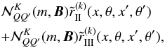$\begin{array}{ccc}& & {\mathrm{𝒩}}_{\mathit{Q}{\mathit{Q}}^{\mathrm{\prime }}}^{\mathit{K}}\mathrm{\left(}\mathit{m,}{B}\mathrm{\right)}\stackrel{}{{{\mathit{r}}_{\mathrm{II}}^{\mathrm{\left(}\mathit{k}\mathrm{\right)}}}_{\mathrm{˜}}}\mathrm{\left(}\mathit{x,\theta ,}{\mathit{x}}^{\mathrm{\prime }}\mathit{,}{\mathit{\theta }}^{\mathrm{\prime }}\mathrm{\right)}\\ & & \end{array}$(26)where the index m ( = 1,2,3,4,5) stands for different (x, x′) frequency domains. The domains relevant to the type-III redistribution are represented by m = 1,2,3 and those relevant to the type-II redistribution by m = 4,5. Expressions for the ${\mathrm{𝒩}}_{\mathit{Q}{\mathit{Q}}^{\mathrm{\prime }}}^{\mathit{K}}\mathrm{\left(}\mathit{m,}{B}\mathrm{\right)}$ can be found in Bommier (1997b, see also Nagendra et al. 2002; Frisch 2007; Anusha et al. 2011).

5. Results and discussions

Here we validate the single scattering approximation presented in Sect. 3, by comparing the solutions computed with this approximation, and those obtained by solving the full radiative transfer equation with an angle-dependent PRD and the Hanle effect. For the latter, we use a perturbation method developed by Nagendra et al. (2002). To obtain the single scattering solution, we first solve the scalar radiative transfer equation with the source term given by Eq. (15), using an ALI method based on the core-wing approach or frequency-angle by frequency-angle approach (see Sampoorna et al. 2011). The scalar intensity ${\mathit{I}}_{\mathrm{0}}^{\mathrm{0}}$ obtained in this way is then used in Eq. (16) or Eqs. (B.1) and (B.2), to compute the single scattered source vector. A formal solution then gives the corresponding single scattered radiation field.

Fig. 1 Comparison of single scattered (dashed lines) and multiple scattered (solid lines) solutions computed with the angle-dependent PRD. A 1D cut-off assumption is used with xc = 3. The model parameters are (a,   ϵ,   r,   ΓE/ΓR) = (10-3,   10-3,   0,   0) and the magnetic field parameters are (Γ,   θB,   χB) = (1,   30°,   0°). The line of sight is represented by μ = 0.11 and χ = 0°. Panel a) corresponds to T = 1, panel b) to T = 100, and panel c) to T = 104.

We consider isothermal, self-emitting plane-parallel atmospheres with no incident radiation at the boundaries. These slab models are characterized by (T,   a,   ϵ,   r,   Γ_E/Γ_R), where T is the optical thickness of the slab and Γ_E is the elastic collisional rate. The depolarizing collisional rate D⁽²⁾ is assumed to be 0.5 × Γ_E. For all the figures presented in this paper, a = 10^-3, ϵ = 10^-3, r = 0 (pure line case), and the line of sight is defined by μ = 0.11 and χ = 0°. The magnetic field parameters are taken as Γ = 1, θ_B = 30°, and χ_B = 0°.

In Fig. 1, we compare the single scattered solution (dashed lines) with the full radiative transfer solution (hereafter, multiple scattered solution; see solid lines) for T = 1 (panel (a)), 100 (panel (b)), and 10⁴ (panel (c)). For brevity, we only show the Q/I and U/I profiles. The comparison is carried out for the type-II angle-dependent redistribution function of Hummer (1962), i.e., with Γ_E/Γ_R = 0. We have used a one-dimensional (1D) cut-off assumption, setting the Hanle effect to zero for x > x_c with x_c = 3. Owing to this abrupt cut-off, spikes or dents are observed around x = 3 (see Fig. 1). Smoother curves can be obtained by using the more realistic 2D domains of Bommier (1997b) (see Fig. 3).

Figure 1 shows that the single scattering approximation can capture the main features of the Q/I and U/I profiles. It is the first time that this approximation has been employed for Stokes U. We can see that it is able to follow the very non-monotonic behavior of U/I. From a quantitative point of view, we observe at line center that the single scattering approximation underestimates the polarization for T = 1 and overestimates it for T = 100 and T = 10⁴. The transition takes place around T = 100. As explained in Frisch et al. (2009) for the case of complete frequency redistribution (CRD), this change in behavior is related to the competition between a limb-darkened outgoing radiation and a limb-brightened incoming one (see also Trujillo Bueno 2001). In the near wings of Q/I, the single scattering approximation strongly underestimates the polarization. We recall that these wings are formed by Rayleigh scattering. For the angle-dependent case, Sampoorna et al. (2011) showed that the exact value of Q/I all along the profile can be obtained by an iterative method incorporating successive scattering orders (see Fig. 5 in this reference). It is likely that this method will also be able to improve the estimation of U/I.

In Fig. 2, we present the single scattered and multiple scattered solutions computed for T = 10⁴, using the more realistic 2D domains of Bommier (1997b). Panel (a) corresponds to the collisionless case and panel (b) to an equal mix of type-II and type-III scattering. We recall that single scattered solutions are calculated with the angle-averaged domains corresponding to approximation-III and the multiple scattered solutions with angle-dependent domains corresponding to approximation-II. Figure 2 shows that this simplifying assumption gives solutions that compare reasonably with the corresponding multiple scattered solutions. The comparison between Figs. 2a and 2b shows that the single scattered solution can become a very good approximation to the multiple scattered solution in the presence of elastic collisions, particularly at the near wing maximum in Q/I profile. For angle-averaged PRD, we also have examples of single scattering solutions providing very accurate approximations (see Fig. 4 of Anusha et al. 2010).

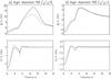Fig. 2 Comparison of single scattered (dashed lines) and multiple scattered (solid lines) solutions computed with approximation-II of Bommier (1997b). The model parameters are (T,   a,   ϵ,   r) = (104,   10-3,   10-3,   0) and the magnetic field parameters are (Γ,   θB,   χB) = (1,   30°,   0°). Panel a) corresponds to collisionless case (ΓE/ΓR = 0) and panel b) to an equal mix of type-II and III scattering (ΓE/ΓR = 1).

The comparison of Fig. 2a with Fig. 1c suggests that U/I is very sensitive to the type of cut-off approximation used. We now discuss this point in more detail. Figure 3 shows the Q/I and U/I profiles computed for the collisionless case, and with three types of frequency domains. The solid lines are computed using a 1D cut-off assumption (x_c = 3), and dashed lines with actual 2D domains of Bommier (1997b). The dotted lines are computed using a square domain (${\mathit{x}}_{\mathrm{c}}\mathrm{=}{\mathit{x}}_{\mathrm{c}}^{\mathrm{\prime }}\mathrm{=}\mathrm{3}$). Such square domains have been used by Fluri et al. (2003, see their Fig. 2b). Figure 3a shows the single scattered solution, while Fig. 3b shows the multiple scattered solution. Clearly Q/I is insensitive to the type of frequency domains used, while U/I is quite sensitive, particularly in the transition region (3 ≤ x < 5).

6. Conclusions

The solution of a polarized line transfer equation with an angle-dependent PRD and the Hanle effect is computationally very demanding. To reduce the complexity of the numerical problem, Frisch (2009) developed a decomposition technique for angle-dependent Hanle problem. In this technique, the non-axisymmetric polarized radiation field is decomposed into an infinite set of cylindrically symmetric Fourier coefficients, by applying an azimuthal Fourier expansion of the angle-dependent PRD function. Such a decomposition method allows one to construct an infinite set of integral equations for the Fourier coefficients of the irreducible source vector components, the solution of which is possible only if we truncate this infinite set. Although the truncated integral equations can be numerically solved, this solution is still computationally demanding (at least 54 integral equations need to be solved simultaneously). Therefore, to simplify the problem, here we have presented an approximate method of solution, based on the single scattering approximation. An approximate solution can be obtained by keeping only the contribution of the zeroth order Fourier coefficient, namely, $\stackrel{}{{{\mathit{I}}_{\mathrm{0}}^{\mathrm{\left(}\mathrm{0}\mathrm{\right)}\mathrm{0}}}_{\mathrm{˜}}}$ in the source terms for the K = 2 components (see Eq. (16)), which are responsible for the generation of Stokes Q and U. As a result, the number of Fourier coefficients reduces to 25 for K = 2 components. The Stokes I in this approximation is assumed to be cylindrically symmetric and decoupled from Stokes Q and U, so that it is computed through a solution of the scalar non-LTE transfer equation with an angle-dependent PRD function. An ALI method associated with a core-wing technique or frequency-angle by frequency-angle technique is used to solve this scalar transfer problem (see Sampoorna et al. 2011).

We have presented the single scattering approximation for a Hanle scattering redistribution matrix with (i) 1D cut-off assumption (see Sect. 3) and (ii) the more realistic frequency domains (see Sect. 4) introduced by Bommier (1997b). We show that the single scattered solution provides a reasonable approximation to the emergent solutions computed by solving the full polarized line transfer equation with angle-dependent PRD and the Hanle effect. To compute the full solution, we use a perturbation method developed by Nagendra et al. (2002). While the perturbation method used by Nagendra et al. (2002) is computationally expensive, the single scattering approximation presented here provides a rapid method of solution. For example, for T = 10⁴ with 41 depth points, seven μ points (eight χ points required only in the case of perturbation method), and 39 frequency points, the perturbation method requires 24 min with 2.7 G Bytes of memory, while single scattered solution can be computed in 20 s with 22 M Bytes of memory, on a Sun Fire V20z Server, 2385 MHz, with a Single-core AMD Opteron processor.

The differences between single scattered and multiple scattered solutions for angle-dependent, as well as angle-averaged PRD are somewhat similar to those for CRD in the line core region. In the case of an angle-dependent and an angle-averaged type-II PRD function, the differences are particularly large at the near wing maximum in Q/I (see Fig. 1c). This difference is reduced in the presence of elastic collisions (see Fig. 2b). Thus, elastic collisions seem to expand the domain of applicability of single scattering approximation. We have also presented the sensitivity of U/I profiles to the choice of different frequency domains (see Fig. 3).

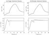Fig. 3 The effect of three types of frequency domains on Q/I and U/I profiles computed using angle-dependent PRD functions. Solid lines correspond to the 1D cut-off assumption (xc = 3), dotted lines to 2D square domains (${\mathit{x}}_{\mathrm{c}}\mathrm{=}{\mathit{x}}_{\mathrm{c}}^{\mathrm{\prime }}\mathrm{=}\mathrm{3}$), and dashed lines to the approximation-II of Bommier (1997b). The model parameters are the same as in Fig. 2a. Panel a) corresponds to single scattered solutions, and panel b) to the multiple scattered solutions.

The single scattered solution presented in this paper can be improved by including higher orders of scattering. Such a method was presented in Frisch et al. (2009) for the Hanle effect with CRD, and in Sampoorna et al. (2011)

for Rayleigh scattering with angle-dependent PRD, where it was referred to as “scattering expansion method”. It is also possible to construct such a scattering expansion method for the case of Hanle effect with an angle-dependent PRD discussed in this paper. The single scattered solution should be seen as an “approximate solution” to the exact solution, and can be used in many practical applications that do not require highly accurate solution of this rather difficult problem, involving angle-dependent PRD matrices.

Online material

Appendix A: The azimuthal Fourier coefficients $\stackrel{}{{{\mathrm{\Gamma }}_{{K}\mathbf{-}{Q}\mathit{,}\mathrm{00}}^{\mathrm{\left(}{Q}\mathrm{\right)}}}_{\mathrm{˜}}}$

The azimuthal Fourier coefficients $\stackrel{}{{{\mathrm{\Gamma }}_{\mathit{KQ,}{\mathit{K}}^{\mathrm{\prime }}{\mathit{Q}}^{\mathrm{\prime }}}^{\mathrm{(}{\mathit{Q}}^{\mathrm{\prime }}\mathrm{-}\mathit{Q}\mathrm{)}}}_{\mathrm{˜}}}$ are defined in Eq. (12). It is easy to verify that they satisfy the properties ${\mathrm{\left[}\stackrel{}{{{\mathrm{\Gamma }}_{\mathit{KQ,}{\mathit{K}}^{\mathrm{\prime }}{\mathit{Q}}^{\mathrm{\prime }}}^{\mathrm{(}{\mathit{Q}}^{\mathrm{\prime }}\mathrm{-}\mathit{Q}\mathrm{)}}}_{\mathrm{˜}}}\mathrm{\right]}}^{\mathrm{\ast }}\mathrm{=}\stackrel{}{{{\mathrm{\Gamma }}_{{\mathit{K}}^{\mathrm{\prime }}{\mathit{Q}}^{\mathrm{\prime }}\mathit{,KQ}}^{\mathrm{(}\mathit{Q}\mathrm{-}{\mathit{Q}}^{\mathrm{\prime }}\mathrm{)}}}_{\mathrm{˜}}}\mathit{,}$(A.1)$\stackrel{}{{{\mathrm{\Gamma }}_{\mathit{K}\mathrm{-}\mathit{Q,}{\mathit{K}}^{\mathrm{\prime }}\mathrm{-}{\mathit{Q}}^{\mathrm{\prime }}}^{\mathrm{(}\mathit{Q}\mathrm{-}{\mathit{Q}}^{\mathrm{\prime }}\mathrm{)}}}_{\mathrm{˜}}}\mathrm{=}\mathrm{(}\mathrm{-}\mathrm{1}{\mathrm{)}}^{\mathit{Q}\mathrm{+}{\mathit{Q}}^{\mathrm{\prime }}}{\mathrm{\left[}\stackrel{}{{{\mathrm{\Gamma }}_{\mathit{KQ,}{\mathit{K}}^{\mathrm{\prime }}{\mathit{Q}}^{\mathrm{\prime }}}^{\mathrm{(}{\mathit{Q}}^{\mathrm{\prime }}\mathrm{-}\mathit{Q}\mathrm{)}}}_{\mathrm{˜}}}\mathrm{\right]}}^{\mathrm{\ast }}\mathit{.}$(A.2)In this Appendix, we give only those Fourier coefficients that are of relevance to the problem at hand, namely those corresponding to K′ = Q′ = 0. Owing to the above-mentioned symmetry relations, there are only four independent coefficients, which are given by $\stackrel{}{{{\mathrm{\Gamma }}_{\mathit{K}\mathrm{-}\mathit{Q,}\mathrm{00}}^{\mathrm{\left(}\mathit{Q}\mathrm{\right)}}}_{\mathrm{˜}}}\mathrm{\left(}\mathit{\theta }\mathrm{\right)}\mathrm{=}\mathrm{(}\mathrm{-}\mathrm{1}{\mathrm{)}}^{\mathit{Q}}\stackrel{}{{{\mathrm{𝒯}}_{\mathit{Q}}^{\mathit{K}}}_{\mathrm{˜}}}\mathrm{(}\mathrm{0}\mathit{,\theta }\mathrm{)}\mathit{.}$(A.3)If we chose the reference angle γ = 0 (see Landi Degl’Innocenti & Landolfi 2004), then from Eq. (A.6) of Frisch (2010), it is clear that $\begin{array}{}{}_{\mathrm{˜}}\\ {\mathrm{𝒯}}_{\mathit{Q}}^{\mathit{K}}\end{array}\mathrm{\left(}\mathrm{0}\mathit{,\theta }\mathrm{\right)}$ are real and hence that $\stackrel{}{{{\mathrm{\Gamma }}_{\mathit{K}\mathrm{-}\mathit{Q,}\mathrm{00}}^{\mathrm{\left(}\mathit{Q}\mathrm{\right)}}}_{\mathrm{˜}}}\mathrm{\left(}\mathit{\theta }\mathrm{\right)}$ are also real. Using Eq. (A.6) of Frisch (2010) in our Eq. (A.3), we obtain the explicit form for these coefficients $\begin{array}{ccc}& & \stackrel{}{{{\mathrm{\Gamma }}_{\mathrm{00}\mathit{,}\mathrm{00}}^{\mathrm{\left(}\mathrm{0}\mathrm{\right)}}}_{\mathrm{˜}}}\mathrm{=}\mathrm{1}\mathrm{;} \stackrel{}{{{\mathrm{\Gamma }}_{\mathrm{20}\mathit{,}\mathrm{00}}^{\mathrm{\left(}\mathrm{0}\mathrm{\right)}}}_{\mathrm{˜}}}\mathrm{=}\frac{\mathrm{1}}{\mathrm{2}\sqrt{\mathrm{2}}}\mathrm{(}\mathrm{3}{\mathit{\mu }}^{\mathrm{2}}\mathrm{-}\mathrm{1}\mathrm{)}\mathit{,}\\ & & \stackrel{}{{{\mathrm{\Gamma }}_{\mathrm{2}\mathrm{-}\mathrm{1}\mathit{,}\mathrm{00}}^{\mathrm{\left(}\mathrm{1}\mathrm{\right)}}}_{\mathrm{˜}}}\mathrm{=}\mathrm{-}\stackrel{}{{{\mathrm{\Gamma }}_{\mathrm{21}\mathit{,}\mathrm{00}}^{\mathrm{(}\mathrm{-}\mathrm{1}\mathrm{)}}}_{\mathrm{˜}}}\mathrm{=}\frac{\sqrt{\mathrm{3}}}{\mathrm{2}}\mathit{\mu }\sqrt{\mathrm{1}\mathrm{-}{\mathit{\mu }}^{\mathrm{2}}}\mathit{,}\\ & & \stackrel{}{{{\mathrm{\Gamma }}_{\mathrm{2}\mathrm{-}\mathrm{2}\mathit{,}\mathrm{00}}^{\mathrm{\left(}\mathrm{2}\mathrm{\right)}}}_{\mathrm{˜}}}\mathrm{=}\stackrel{}{{{\mathrm{\Gamma }}_{\mathrm{22}\mathit{,}\mathrm{00}}^{\mathrm{(}\mathrm{-}\mathrm{2}\mathrm{)}}}_{\mathrm{˜}}}\mathrm{=}\frac{\sqrt{\mathrm{3}}}{\mathrm{4}}\mathrm{(}\mathrm{1}\mathrm{-}{\mathit{\mu }}^{\mathrm{2}}\mathrm{)}\mathit{.}\end{array}$(A.4)

Appendix B: The explicit form of the real components of $\stackrel{}{{{\mathit{S}}_{{l,Q}}^{\mathrm{\left(}{k}\mathrm{\right)}\mathrm{2}}}_{\mathrm{˜}}}$

In this Appendix, we list the explicit analytic forms of the 25 non-zero real components of $\stackrel{}{{{\mathit{S}}_{\mathit{l,Q}}^{\mathrm{\left(}\mathit{k}\mathrm{\right)}\mathrm{2}}}_{\mathrm{˜}}}$, defined in Eqs. (19), (20), and (25) of the text. For K = 2, we define ${\mathit{Z}}_{\mathrm{2}\mathrm{-}\mathit{k}}^{\mathrm{\left(}\mathit{k}\mathrm{\right)}}\mathrm{=}\frac{\mathrm{1}}{\mathrm{2}}{\mathrm{\int }}_{\mathrm{-}\mathrm{\infty }}^{\mathrm{+}\mathrm{\infty }}{\mathrm{\int }}_{\mathrm{0}}^{\mathit{\pi }}\frac{\stackrel{}{{{\mathit{r}}^{\mathrm{\left(}\mathit{k}\mathrm{\right)}}}_{\mathrm{˜}}}\mathrm{\left(}\mathit{x,\theta ,}{\mathit{x}}^{\mathrm{\prime }}\mathit{,}{\mathit{\theta }}^{\mathrm{\prime }}\mathrm{\right)}}{\mathit{\varphi }\mathrm{\left(}\mathit{x}\mathrm{\right)}}\stackrel{}{{{\mathrm{\Gamma }}_{\mathrm{2}\mathrm{-}\mathit{k,}\mathrm{00}}^{\mathrm{\left(}\mathit{k}\mathrm{\right)}}}_{\mathrm{˜}}}\mathrm{\left(}{\mathit{\theta }}^{\mathrm{\prime }}\mathrm{\right)}{\mathit{I}}_{\mathrm{0}}^{\mathrm{0}}\mathrm{\left(}\mathit{\tau ,}{\mathit{x}}^{\mathrm{\prime }}\mathit{,}{\mathit{\theta }}^{\mathrm{\prime }}\mathrm{\right)}\sin {\mathit{\theta }}^{\mathrm{\prime }}\hspace{0.17em}\mathrm{d}{\mathit{\theta }}^{\mathrm{\prime }}\hspace{0.17em}\mathrm{d}{\mathit{x}}^{\mathrm{\prime }}\mathit{.}$(B.1)We can express all the 25 non-zero real components of $\stackrel{}{{{\mathit{S}}_{\mathit{l,Q}}^{\mathrm{\left(}\mathit{k}\mathrm{\right)}\mathrm{2}}}_{\mathrm{˜}}}$ in terms of ${\mathit{Z}}_{\mathrm{2}\mathrm{-}\mathit{k}}^{\mathrm{\left(}\mathit{k}\mathrm{\right)}}$ as follows : $\begin{array}{ccc}\stackrel{}{{{\mathit{S}}_{\mathit{l,}\mathrm{0}}^{\mathrm{x}\mathrm{\left(}\mathrm{0}\mathrm{\right)}\mathrm{2}}}_{\mathrm{˜}}}& \mathrm{=}& \mathrm{\Re }\mathrm{\left[}{\mathrm{𝒩}}_{\mathrm{00}}^{\mathrm{2}}\mathrm{\right]}\hspace{0.17em}{\mathit{Z}}_{\mathrm{20}}^{\mathrm{\left(}\mathrm{0}\mathrm{\right)}}\mathrm{;} \hspace{0.17em}\stackrel{}{{{\mathit{S}}_{\mathit{l,}\mathrm{0}}^{\mathrm{x}\mathrm{\left(}\mathrm{1}\mathrm{\right)}\mathrm{2}}}_{\mathrm{˜}}}\mathrm{=}\mathrm{\Re }\mathrm{\left[}{\mathrm{𝒩}}_{\mathrm{0}\mathrm{-}\mathrm{1}}^{\mathrm{2}}\mathrm{\right]}\hspace{0.17em}{\mathit{Z}}_{\mathrm{2}\mathrm{-}\mathrm{1}}^{\mathrm{\left(}\mathrm{1}\mathrm{\right)}}\mathit{,}\\ \stackrel{}{{{\mathit{S}}_{\mathit{l,}\mathrm{0}}^{\mathrm{x}\mathrm{\left(}\mathrm{2}\mathrm{\right)}\mathrm{2}}}_{\mathrm{˜}}}& \mathrm{=}& \mathrm{\Re }\mathrm{\left[}{\mathrm{𝒩}}_{\mathrm{0}\mathrm{-}\mathrm{2}}^{\mathrm{2}}\mathrm{\right]}\hspace{0.17em}{\mathit{Z}}_{\mathrm{2}\mathrm{-}\mathrm{2}}^{\mathrm{\left(}\mathrm{2}\mathrm{\right)}}\mathrm{;} \hspace{0.17em}\stackrel{}{{{\mathit{S}}_{\mathit{l,}\mathrm{0}}^{\mathrm{y}\mathrm{\left(}\mathrm{1}\mathrm{\right)}\mathrm{2}}}_{\mathrm{˜}}}\mathrm{=}\mathrm{\Im }\mathrm{\left[}{\mathrm{𝒩}}_{\mathrm{0}\mathrm{-}\mathrm{1}}^{\mathrm{2}}\mathrm{\right]}\hspace{0.17em}{\mathit{Z}}_{\mathrm{2}\mathrm{-}\mathrm{1}}^{\mathrm{\left(}\mathrm{1}\mathrm{\right)}}\mathit{,}\\ \stackrel{}{{{\mathit{S}}_{\mathit{l,}\mathrm{0}}^{\mathrm{y}\mathrm{\left(}\mathrm{2}\mathrm{\right)}\mathrm{2}}}_{\mathrm{˜}}}& \mathrm{=}& \mathrm{\Im }\mathrm{\left[}{\mathrm{𝒩}}_{\mathrm{0}\mathrm{-}\mathrm{2}}^{\mathrm{2}}\mathrm{\right]}\hspace{0.17em}{\mathit{Z}}_{\mathrm{2}\mathrm{-}\mathrm{2}}^{\mathrm{\left(}\mathrm{2}\mathrm{\right)}}\mathrm{;} \hspace{0.17em}\stackrel{}{{{\mathit{S}}_{\mathit{l,}\mathrm{1}}^{\mathrm{x}\mathrm{\left(}\mathrm{0}\mathrm{\right)}\mathrm{2}}}_{\mathrm{˜}}}\mathrm{=}\mathrm{\Re }\mathrm{\left[}{\mathrm{𝒩}}_{\mathrm{10}}^{\mathrm{2}}\mathrm{\right]}\hspace{0.17em}{\mathit{Z}}_{\mathrm{20}}^{\mathrm{\left(}\mathrm{0}\mathrm{\right)}}\mathit{,}\\ \stackrel{}{{{\mathit{S}}_{\mathit{l,}\mathrm{1}}^{\mathrm{x}\mathrm{+}\mathrm{\left(}\mathrm{1}\mathrm{\right)}\mathrm{2}}}_{\mathrm{˜}}}& \mathrm{=}& \frac{\mathrm{1}}{\mathrm{2}}\mathrm{\Re }\mathrm{[}{\mathrm{𝒩}}_{\mathrm{1}\mathrm{-}\mathrm{1}}^{\mathrm{2}}\mathrm{-}{\mathrm{𝒩}}_{\mathrm{11}}^{\mathrm{2}}\mathrm{]}\hspace{0.17em}{\mathit{Z}}_{\mathrm{2}\mathrm{-}\mathrm{1}}^{\mathrm{\left(}\mathrm{1}\mathrm{\right)}}\mathrm{;} \stackrel{}{{{\mathit{S}}_{\mathit{l,}\mathrm{1}}^{\mathrm{x}\mathrm{+}\mathrm{\left(}\mathrm{2}\mathrm{\right)}\mathrm{2}}}_{\mathrm{˜}}}\mathrm{=}\frac{\mathrm{1}}{\mathrm{2}}\mathrm{\Re }\mathrm{[}{\mathrm{𝒩}}_{\mathrm{1}\mathrm{-}\mathrm{2}}^{\mathrm{2}}\mathrm{+}{\mathrm{𝒩}}_{\mathrm{12}}^{\mathrm{2}}\mathrm{]}\hspace{0.17em}{\mathit{Z}}_{\mathrm{2}\mathrm{-}\mathrm{2}}^{\mathrm{\left(}\mathrm{2}\mathrm{\right)}}\mathit{,}\\ \stackrel{}{{{\mathit{S}}_{\mathit{l,}\mathrm{1}}^{\mathrm{y}\mathrm{-}\mathrm{\left(}\mathrm{1}\mathrm{\right)}\mathrm{2}}}_{\mathrm{˜}}}& \mathrm{=}& \mathrm{-}\frac{\mathrm{1}}{\mathrm{2}}\mathrm{\Im }\mathrm{[}{\mathrm{𝒩}}_{\mathrm{11}}^{\mathrm{2}}\mathrm{+}{\mathrm{𝒩}}_{\mathrm{1}\mathrm{-}\mathrm{1}}^{\mathrm{2}}\mathrm{]}\hspace{0.17em}{\mathit{Z}}_{\mathrm{2}\mathrm{-}\mathrm{1}}^{\mathrm{\left(}\mathrm{1}\mathrm{\right)}}\mathrm{;} \hspace{0.17em}\stackrel{}{{{\mathit{S}}_{\mathit{l,}\mathrm{1}}^{\mathrm{y}\mathrm{-}\mathrm{\left(}\mathrm{2}\mathrm{\right)}\mathrm{2}}}_{\mathrm{˜}}}\mathrm{=}\frac{\mathrm{1}}{\mathrm{2}}\mathrm{\Im }\mathrm{[}{\mathrm{𝒩}}_{\mathrm{12}}^{\mathrm{2}}\mathrm{-}{\mathrm{𝒩}}_{\mathrm{1}\mathrm{-}\mathrm{2}}^{\mathrm{2}}\mathrm{]}\hspace{0.17em}{\mathit{Z}}_{\mathrm{2}\mathrm{-}\mathrm{2}}^{\mathrm{\left(}\mathrm{2}\mathrm{\right)}}\mathit{,}\\ \stackrel{}{{{\mathit{S}}_{\mathit{l,}\mathrm{2}}^{\mathrm{x}\mathrm{\left(}\mathrm{0}\mathrm{\right)}\mathrm{2}}}_{\mathrm{˜}}}& \mathrm{=}& \mathrm{\Re }\mathrm{\left[}{\mathrm{𝒩}}_{\mathrm{20}}^{\mathrm{2}}\mathrm{\right]}\hspace{0.17em}{\mathit{Z}}_{\mathrm{20}}^{\mathrm{\left(}\mathrm{0}\mathrm{\right)}}\mathrm{;} \hspace{0.17em}\stackrel{}{{{\mathit{S}}_{\mathit{l,}\mathrm{2}}^{\mathrm{x}\mathrm{+}\mathrm{\left(}\mathrm{1}\mathrm{\right)}\mathrm{2}}}_{\mathrm{˜}}}\mathrm{=}\frac{\mathrm{1}}{\mathrm{2}}\mathrm{\Re }\mathrm{[}{\mathrm{𝒩}}_{\mathrm{2}\mathrm{-}\mathrm{1}}^{\mathrm{2}}\mathrm{-}{\mathrm{𝒩}}_{\mathrm{21}}^{\mathrm{2}}\mathrm{]}\hspace{0.17em}{\mathit{Z}}_{\mathrm{2}\mathrm{-}\mathrm{1}}^{\mathrm{\left(}\mathrm{1}\mathrm{\right)}}\mathit{,}\\ \stackrel{}{{{\mathit{S}}_{\mathit{l,}\mathrm{2}}^{\mathrm{x}\mathrm{+}\mathrm{\left(}\mathrm{2}\mathrm{\right)}\mathrm{2}}}_{\mathrm{˜}}}& \mathrm{=}& \frac{\mathrm{1}}{\mathrm{2}}\mathrm{\Re }\mathrm{[}{\mathrm{𝒩}}_{\mathrm{2}\mathrm{-}\mathrm{2}}^{\mathrm{2}}\mathrm{+}{\mathrm{𝒩}}_{\mathrm{22}}^{\mathrm{2}}\mathrm{]}\hspace{0.17em}{\mathit{Z}}_{\mathrm{2}\mathrm{-}\mathrm{2}}^{\mathrm{\left(}\mathrm{2}\mathrm{\right)}}\mathrm{;} \stackrel{}{{{\mathit{S}}_{\mathit{l,}\mathrm{2}}^{\mathrm{y}\mathrm{-}\mathrm{\left(}\mathrm{1}\mathrm{\right)}\mathrm{2}}}_{\mathrm{˜}}}\mathrm{=}\mathrm{-}\frac{\mathrm{1}}{\mathrm{2}}\mathrm{\Im }\mathrm{[}{\mathrm{𝒩}}_{\mathrm{21}}^{\mathrm{2}}\mathrm{+}{\mathrm{𝒩}}_{\mathrm{2}\mathrm{-}\mathrm{1}}^{\mathrm{2}}\mathrm{]}\hspace{0.17em}{\mathit{Z}}_{\mathrm{2}\mathrm{-}\mathrm{1}}^{\mathrm{\left(}\mathrm{1}\mathrm{\right)}}\mathit{,}\\ \stackrel{}{{{\mathit{S}}_{\mathit{l,}\mathrm{2}}^{\mathrm{y}\mathrm{-}\mathrm{\left(}\mathrm{2}\mathrm{\right)}\mathrm{2}}}_{\mathrm{˜}}}& \mathrm{=}& \frac{\mathrm{1}}{\mathrm{2}}\mathrm{\Im }\mathrm{[}{\mathrm{𝒩}}_{\mathrm{22}}^{\mathrm{2}}\mathrm{-}{\mathrm{𝒩}}_{\mathrm{2}\mathrm{-}\mathrm{2}}^{\mathrm{2}}\mathrm{]}\hspace{0.17em}{\mathit{Z}}_{\mathrm{2}\mathrm{-}\mathrm{2}}^{\mathrm{\left(}\mathrm{2}\mathrm{\right)}}\mathrm{;} \hspace{0.17em}\hspace{0.17em}\stackrel{}{{{\mathit{S}}_{\mathit{l,}\mathrm{1}}^{\mathrm{y}\mathrm{\left(}\mathrm{0}\mathrm{\right)}\mathrm{2}}}_{\mathrm{˜}}}\mathrm{=}\mathrm{\Im }\mathrm{\left[}{\mathrm{𝒩}}_{\mathrm{10}}^{\mathrm{2}}\mathrm{\right]}\hspace{0.17em}{\mathit{Z}}_{\mathrm{20}}^{\mathrm{\left(}\mathrm{0}\mathrm{\right)}}\mathit{,}\\ \stackrel{}{{{\mathit{S}}_{\mathit{l,}\mathrm{1}}^{\mathrm{y}\mathrm{+}\mathrm{\left(}\mathrm{1}\mathrm{\right)}\mathrm{2}}}_{\mathrm{˜}}}& \mathrm{=}& \frac{\mathrm{1}}{\mathrm{2}}\mathrm{\Im }\mathrm{[}{\mathrm{𝒩}}_{\mathrm{1}\mathrm{-}\mathrm{1}}^{\mathrm{2}}\mathrm{-}{\mathrm{𝒩}}_{\mathrm{11}}^{\mathrm{2}}\mathrm{]}\hspace{0.17em}{\mathit{Z}}_{\mathrm{2}\mathrm{-}\mathrm{1}}^{\mathrm{\left(}\mathrm{1}\mathrm{\right)}}\mathrm{;} \hspace{0.17em}\hspace{0.17em}\stackrel{}{{{\mathit{S}}_{\mathit{l,}\mathrm{1}}^{\mathrm{y}\mathrm{+}\mathrm{\left(}\mathrm{2}\mathrm{\right)}\mathrm{2}}}_{\mathrm{˜}}}\mathrm{=}\frac{\mathrm{1}}{\mathrm{2}}\mathrm{\Im }\mathrm{[}{\mathrm{𝒩}}_{\mathrm{1}\mathrm{-}\mathrm{2}}^{\mathrm{2}}\mathrm{+}{\mathrm{𝒩}}_{\mathrm{12}}^{\mathrm{2}}\mathrm{]}\hspace{0.17em}{\mathit{Z}}_{\mathrm{2}\mathrm{-}\mathrm{2}}^{\mathrm{\left(}\mathrm{2}\mathrm{\right)}}\mathit{,}\\ \stackrel{}{{{\mathit{S}}_{\mathit{l,}\mathrm{1}}^{\mathrm{x}\mathrm{-}\mathrm{\left(}\mathrm{1}\mathrm{\right)}\mathrm{2}}}_{\mathrm{˜}}}& \mathrm{=}& \frac{\mathrm{1}}{\mathrm{2}}\mathrm{\Re }\mathrm{[}{\mathrm{𝒩}}_{\mathrm{1}\mathrm{-}\mathrm{1}}^{\mathrm{2}}\mathrm{+}{\mathrm{𝒩}}_{\mathrm{11}}^{\mathrm{2}}\mathrm{]}\hspace{0.17em}{\mathit{Z}}_{\mathrm{2}\mathrm{-}\mathrm{1}}^{\mathrm{\left(}\mathrm{1}\mathrm{\right)}}\mathrm{;} \stackrel{}{{{\mathit{S}}_{\mathit{l,}\mathrm{1}}^{\mathrm{x}\mathrm{-}\mathrm{\left(}\mathrm{2}\mathrm{\right)}\mathrm{2}}}_{\mathrm{˜}}}\mathrm{=}\frac{\mathrm{1}}{\mathrm{2}}\mathrm{\Re }\mathrm{[}{\mathrm{𝒩}}_{\mathrm{1}\mathrm{-}\mathrm{2}}^{\mathrm{2}}\mathrm{-}{\mathrm{𝒩}}_{\mathrm{12}}^{\mathrm{2}}\mathrm{]}\hspace{0.17em}{\mathit{Z}}_{\mathrm{2}\mathrm{-}\mathrm{2}}^{\mathrm{\left(}\mathrm{2}\mathrm{\right)}}\mathit{,}\\ \stackrel{}{{{\mathit{S}}_{\mathit{l,}\mathrm{2}}^{\mathrm{y}\mathrm{\left(}\mathrm{0}\mathrm{\right)}\mathrm{2}}}_{\mathrm{˜}}}& \mathrm{=}& \mathrm{\Im }\mathrm{\left[}{\mathrm{𝒩}}_{\mathrm{20}}^{\mathrm{2}}\mathrm{\right]}\hspace{0.17em}{\mathit{Z}}_{\mathrm{20}}^{\mathrm{\left(}\mathrm{0}\mathrm{\right)}}\mathrm{;} \hspace{0.17em}\stackrel{}{{{\mathit{S}}_{\mathit{l,}\mathrm{2}}^{\mathrm{y}\mathrm{+}\mathrm{\left(}\mathrm{1}\mathrm{\right)}\mathrm{2}}}_{\mathrm{˜}}}\mathrm{=}\frac{\mathrm{1}}{\mathrm{2}}\mathrm{\Im }\mathrm{[}{\mathrm{𝒩}}_{\mathrm{2}\mathrm{-}\mathrm{1}}^{\mathrm{2}}\mathrm{-}{\mathrm{𝒩}}_{\mathrm{21}}^{\mathrm{2}}\mathrm{]}\hspace{0.17em}{\mathit{Z}}_{\mathrm{2}\mathrm{-}\mathrm{1}}^{\mathrm{\left(}\mathrm{1}\mathrm{\right)}}\mathit{,}\\ \stackrel{}{{{\mathit{S}}_{\mathit{l,}\mathrm{2}}^{\mathrm{y}\mathrm{+}\mathrm{\left(}\mathrm{2}\mathrm{\right)}\mathrm{2}}}_{\mathrm{˜}}}& \mathrm{=}& \frac{\mathrm{1}}{\mathrm{2}}\mathrm{\Im }\mathrm{[}{\mathrm{𝒩}}_{\mathrm{2}\mathrm{-}\mathrm{2}}^{\mathrm{2}}\mathrm{+}{\mathrm{𝒩}}_{\mathrm{22}}^{\mathrm{2}}\mathrm{]}\hspace{0.17em}{\mathit{Z}}_{\mathrm{2}\mathrm{-}\mathrm{2}}^{\mathrm{\left(}\mathrm{2}\mathrm{\right)}}\mathrm{;} \stackrel{}{{{\mathit{S}}_{\mathit{l,}\mathrm{2}}^{\mathrm{x}\mathrm{-}\mathrm{\left(}\mathrm{1}\mathrm{\right)}\mathrm{2}}}_{\mathrm{˜}}}\mathrm{=}\frac{\mathrm{1}}{\mathrm{2}}\mathrm{\Re }\mathrm{[}{\mathrm{𝒩}}_{\mathrm{2}\mathrm{-}\mathrm{1}}^{\mathrm{2}}\mathrm{+}{\mathrm{𝒩}}_{\mathrm{21}}^{\mathrm{2}}\mathrm{]}\hspace{0.17em}{\mathit{Z}}_{\mathrm{2}\mathrm{-}\mathrm{1}}^{\mathrm{\left(}\mathrm{1}\mathrm{\right)}}\mathit{,}\\ \stackrel{}{{{\mathit{S}}_{\mathit{l,}\mathrm{2}}^{\mathrm{x}\mathrm{-}\mathrm{\left(}\mathrm{2}\mathrm{\right)}\mathrm{2}}}_{\mathrm{˜}}}& \mathrm{=}& \end{array}$(B.2)The above equations are valid for x < x_c in the case of a 1D cut-off assumption. For x > x_c, we have to set ${\mathrm{𝒩}}_{\mathit{Q}\mathrm{-}\mathit{k}}^{\mathrm{2}}\mathrm{=}{\mathit{W}}_{\mathrm{2}}\mathrm{(}\mathrm{1}\mathrm{-}\mathit{ϵ}\mathrm{)}{\mathit{\delta }}_{\mathit{Q}\mathrm{-}\mathit{k}}$. In the case of approximation-II, the various ${\mathrm{𝒩}}_{\mathit{Q}\mathrm{-}\mathit{k}}^{\mathrm{2}}$ appearing in the above equations should be taken inside the frequency integral appearing in Eq. (B.1), and Eqs. (106)–(113) of Bommier (1997b) have to be used.

The various ${\mathrm{𝒩}}_{\mathit{Q}\mathrm{-}\mathit{k}}^{\mathrm{2}}$ appearing in the above set of equations are given by Eq. (6) in the case of the 1D cut-off assumption and Eqs. (A11)–(A18) of Anusha et al. (in press) in the case of the 2D frequency domains of Bommier (1997b). Below we give the explicit forms of ${\mathrm{ℳ}}_{\mathit{Q}{\mathit{Q}}^{\mathrm{\prime }}}^{\mathit{K}}\mathrm{\left(}{\mathit{\theta }}_{\mathit{B}}\mathit{,}{\mathit{\chi }}_{\mathit{B}}\mathit{,}\mathrm{\Gamma }\mathrm{\right)}$ appearing in those equations. We introduce the abbreviations, C_B = cosθ_B, S_B = sinθ_B, c₁ = cosχ_B, s₁ = sinχ_B, c₂ = cos2χ_B, and s₂ = sin2χ_B. In terms of the elements of the matrix given below (see also Appendix C in Frisch 2007), we have $\begin{array}{ccc}\mathrm{\Re }\mathrm{\left[}{\mathrm{ℳ}}_{\mathrm{00}}^{\mathrm{2}}\mathrm{\right]}\mathrm{=}{\mathit{m}}_{\mathrm{11}}& \mathrm{=}& \mathrm{1}\mathrm{-}\mathrm{3}{\mathit{S}}_{\mathit{B}}^{\mathrm{2}}{\mathrm{\Gamma }}^{\mathrm{2}}\left[\frac{{\mathit{C}}_{\mathit{B}}^{\mathrm{2}}}{\mathrm{1}\mathrm{+}{\mathrm{\Gamma }}^{\mathrm{2}}}\mathrm{+}\frac{{\mathit{S}}_{\mathit{B}}^{\mathrm{2}}}{\mathrm{1}\mathrm{+}\mathrm{4}{\mathrm{\Gamma }}^{\mathrm{2}}}\right]\mathrm{;} \mathrm{\Re }\mathrm{[}{\mathrm{ℳ}}_{\mathrm{1}\mathrm{-}\mathrm{1}}^{\mathrm{2}}\mathrm{-}{\mathrm{ℳ}}_{\mathrm{11}}^{\mathrm{2}}\mathrm{]}\mathrm{=}\mathrm{-}{\mathit{c}}_{\mathrm{1}}^{\mathrm{2}}{\mathit{m}}_{\mathrm{22}}\mathrm{-}{\mathit{s}}_{\mathrm{1}}^{\mathrm{2}}{\mathit{m}}_{\mathrm{33}}\mathit{,}\\ \mathrm{\Re }\mathrm{[}{\mathrm{ℳ}}_{\mathrm{1}\mathrm{-}\mathrm{2}}^{\mathrm{2}}\mathrm{+}{\mathrm{ℳ}}_{\mathrm{12}}^{\mathrm{2}}\mathrm{]}& \mathrm{=}& {\mathit{c}}_{\mathrm{1}}{\mathit{c}}_{\mathrm{2}}{\mathit{m}}_{\mathrm{24}}\mathrm{+}{\mathit{s}}_{\mathrm{1}}{\mathit{s}}_{\mathrm{2}}{\mathit{m}}_{\mathrm{35}}\mathrm{+}{\mathit{s}}_{\mathrm{2}}{\mathit{c}}_{\mathrm{1}}{\mathit{m}}_{\mathrm{25}}\mathrm{+}{\mathit{c}}_{\mathrm{2}}{\mathit{s}}_{\mathrm{1}}{\mathit{m}}_{\mathrm{34}}\mathrm{;} \mathrm{\Re }\mathrm{\left[}{\mathrm{ℳ}}_{\mathrm{0}\mathrm{-}\mathrm{1}}^{\mathrm{2}}\mathrm{\right]}\mathrm{=}\mathrm{-}{\mathit{c}}_{\mathrm{1}}{\mathit{m}}_{\mathrm{12}}\mathrm{-}{\mathit{s}}_{\mathrm{1}}{\mathit{m}}_{\mathrm{13}}\mathit{,}\\ \mathrm{-}\mathrm{\Im }\mathrm{[}{\mathrm{ℳ}}_{\mathrm{11}}^{\mathrm{2}}\mathrm{+}{\mathrm{ℳ}}_{\mathrm{1}\mathrm{-}\mathrm{1}}^{\mathrm{2}}\mathrm{]}& \mathrm{=}& \mathrm{(}{\mathit{c}}_{\mathrm{1}}^{\mathrm{2}}\mathrm{+}{\mathit{s}}_{\mathrm{1}}^{\mathrm{2}}\mathrm{)}{\mathit{m}}_{\mathrm{23}}\mathrm{-}{\mathit{c}}_{\mathrm{1}}{\mathit{s}}_{\mathrm{1}}\mathrm{(}{\mathit{m}}_{\mathrm{22}}\mathrm{-}{\mathit{m}}_{\mathrm{33}}\mathrm{)}\mathrm{;} \mathrm{\Re }\mathrm{\left[}{\mathrm{ℳ}}_{\mathrm{0}\mathrm{-}\mathrm{2}}^{\mathrm{2}}\mathrm{\right]}\mathrm{=}{\mathit{c}}_{\mathrm{2}}{\mathit{m}}_{\mathrm{14}}\mathrm{+}{\mathit{s}}_{\mathrm{2}}{\mathit{m}}_{\mathrm{15}}\mathrm{;}\\ \mathrm{\Im }\mathrm{[}{\mathrm{ℳ}}_{\mathrm{12}}^{\mathrm{2}}\mathrm{-}{\mathrm{ℳ}}_{\mathrm{1}\mathrm{-}\mathrm{2}}^{\mathrm{2}}\mathrm{]}& \mathrm{=}& {\mathit{s}}_{\mathrm{2}}{\mathit{c}}_{\mathrm{1}}{\mathit{m}}_{\mathrm{24}}\mathrm{-}{\mathit{c}}_{\mathrm{2}}{\mathit{s}}_{\mathrm{1}}{\mathit{m}}_{\mathrm{35}}\mathrm{-}{\mathit{c}}_{\mathrm{1}}{\mathit{c}}_{\mathrm{2}}{\mathit{m}}_{\mathrm{25}}\mathrm{+}{\mathit{s}}_{\mathrm{1}}{\mathit{s}}_{\mathrm{2}}{\mathit{m}}_{\mathrm{34}}\mathrm{;} \mathrm{\Im }\mathrm{\left[}{\mathrm{ℳ}}_{\mathrm{0}\mathrm{-}\mathrm{1}}^{\mathrm{2}}\mathrm{\right]}\mathrm{=}{\mathit{s}}_{\mathrm{1}}{\mathit{m}}_{\mathrm{12}}\mathrm{-}{\mathit{c}}_{\mathrm{1}}{\mathit{m}}_{\mathrm{13}}\mathit{,}\\ \mathrm{\Re }\mathrm{[}{\mathrm{ℳ}}_{\mathrm{2}\mathrm{-}\mathrm{1}}^{\mathrm{2}}\mathrm{-}{\mathrm{ℳ}}_{\mathrm{21}}^{\mathrm{2}}\mathrm{]}& \mathrm{=}& \mathrm{-}{\mathit{c}}_{\mathrm{1}}{\mathit{c}}_{\mathrm{2}}{\mathit{m}}_{\mathrm{24}}\mathrm{-}{\mathit{s}}_{\mathrm{1}}{\mathit{s}}_{\mathrm{2}}{\mathit{m}}_{\mathrm{35}}\mathrm{+}{\mathit{s}}_{\mathrm{2}}{\mathit{c}}_{\mathrm{1}}{\mathit{m}}_{\mathrm{25}}\mathrm{+}{\mathit{c}}_{\mathrm{2}}{\mathit{s}}_{\mathrm{1}}{\mathit{m}}_{\mathrm{34}}\mathrm{;} \mathrm{\Im }\mathrm{\left[}{\mathrm{ℳ}}_{\mathrm{0}\mathrm{-}\mathrm{2}}^{\mathrm{2}}\mathrm{\right]}\mathrm{=}\mathrm{-}{\mathit{s}}_{\mathrm{2}}{\mathit{m}}_{\mathrm{14}}\mathrm{+}{\mathit{c}}_{\mathrm{2}}{\mathit{m}}_{\mathrm{15}}\mathit{,}\\ \mathrm{\Im }\mathrm{[}{\mathrm{ℳ}}_{\mathrm{1}\mathrm{-}\mathrm{2}}^{\mathrm{2}}\mathrm{+}{\mathrm{ℳ}}_{\mathrm{12}}^{\mathrm{2}}\mathrm{]}& \mathrm{=}& {\mathit{s}}_{\mathrm{2}}{\mathit{c}}_{\mathrm{1}}{\mathit{m}}_{\mathrm{35}}\mathrm{-}{\mathit{c}}_{\mathrm{2}}{\mathit{s}}_{\mathrm{1}}{\mathit{m}}_{\mathrm{24}}\mathrm{+}{\mathit{c}}_{\mathrm{1}}{\mathit{c}}_{\mathrm{2}}{\mathit{m}}_{\mathrm{34}}\mathrm{-}{\mathit{s}}_{\mathrm{1}}{\mathit{s}}_{\mathrm{2}}{\mathit{m}}_{\mathrm{25}}\mathrm{;} \mathrm{\Re }\mathrm{\left[}{\mathrm{ℳ}}_{\mathrm{10}}^{\mathrm{2}}\mathrm{\right]}\mathrm{=}{\mathit{c}}_{\mathrm{1}}{\mathit{m}}_{\mathrm{12}}\mathrm{-}{\mathit{s}}_{\mathrm{1}}{\mathit{m}}_{\mathrm{13}}\mathit{,}\\ \mathrm{-}\mathrm{\Im }\mathrm{[}{\mathrm{ℳ}}_{\mathrm{21}}^{\mathrm{2}}\mathrm{+}{\mathrm{ℳ}}_{\mathrm{2}\mathrm{-}\mathrm{1}}^{\mathrm{2}}\mathrm{]}& \mathrm{=}& {\mathit{s}}_{\mathrm{2}}{\mathit{c}}_{\mathrm{1}}{\mathit{m}}_{\mathrm{35}}\mathrm{-}{\mathit{c}}_{\mathrm{2}}{\mathit{s}}_{\mathrm{1}}{\mathit{m}}_{\mathrm{24}}\mathrm{-}{\mathit{c}}_{\mathrm{1}}{\mathit{c}}_{\mathrm{2}}{\mathit{m}}_{\mathrm{34}}\mathrm{+}{\mathit{s}}_{\mathrm{1}}{\mathit{s}}_{\mathrm{2}}{\mathit{m}}_{\mathrm{25}}\mathrm{;} \mathrm{\Re }\mathrm{\left[}{\mathrm{ℳ}}_{\mathrm{20}}^{\mathrm{2}}\mathrm{\right]}\mathrm{=}{\mathit{c}}_{\mathrm{2}}{\mathit{m}}_{\mathrm{14}}\mathrm{-}{\mathit{s}}_{\mathrm{2}}{\mathit{m}}_{\mathrm{15}}\mathit{,}\\ \mathrm{\Im }\mathrm{[}{\mathrm{ℳ}}_{\mathrm{22}}^{\mathrm{2}}\mathrm{-}{\mathrm{ℳ}}_{\mathrm{2}\mathrm{-}\mathrm{2}}^{\mathrm{2}}\mathrm{]}& \mathrm{=}& \mathrm{-}\mathrm{(}{\mathit{c}}_{\mathrm{2}}^{\mathrm{2}}\mathrm{+}{\mathit{s}}_{\mathrm{2}}^{\mathrm{2}}\mathrm{)}{\mathit{m}}_{\mathrm{45}}\mathrm{+}{\mathit{c}}_{\mathrm{2}}{\mathit{s}}_{\mathrm{2}}\mathrm{(}{\mathit{m}}_{\mathrm{44}}\mathrm{-}{\mathit{m}}_{\mathrm{55}}\mathrm{)}\mathrm{;} \mathrm{\Im }\mathrm{\left[}{\mathrm{ℳ}}_{\mathrm{10}}^{\mathrm{2}}\mathrm{\right]}\mathrm{=}\mathrm{-}{\mathit{s}}_{\mathrm{1}}{\mathit{m}}_{\mathrm{12}}\mathrm{-}{\mathit{c}}_{\mathrm{1}}{\mathit{m}}_{\mathrm{13}}\mathit{,}\\ \mathrm{\Im }\mathrm{[}{\mathrm{ℳ}}_{\mathrm{1}\mathrm{-}\mathrm{1}}^{\mathrm{2}}\mathrm{-}{\mathrm{ℳ}}_{\mathrm{11}}^{\mathrm{2}}\mathrm{]}& \mathrm{=}& \mathrm{(}{\mathit{c}}_{\mathrm{1}}^{\mathrm{2}}\mathrm{+}{\mathit{s}}_{\mathrm{1}}^{\mathrm{2}}\mathrm{)}{\mathit{m}}_{\mathrm{23}}\mathrm{+}{\mathit{c}}_{\mathrm{1}}{\mathit{s}}_{\mathrm{1}}\mathrm{(}{\mathit{m}}_{\mathrm{22}}\mathrm{-}{\mathit{m}}_{\mathrm{33}}\mathrm{)}\mathrm{;} \hspace{0.17em}\mathrm{\Re }\mathrm{[}{\mathrm{ℳ}}_{\mathrm{2}\mathrm{-}\mathrm{2}}^{\mathrm{2}}\mathrm{+}{\mathrm{ℳ}}_{\mathrm{22}}^{\mathrm{2}}\mathrm{]}\mathrm{=}{\mathit{c}}_{\mathrm{2}}^{\mathrm{2}}{\mathit{m}}_{\mathrm{44}}\mathrm{+}{\mathit{s}}_{\mathrm{2}}^{\mathrm{2}}{\mathit{m}}_{\mathrm{55}}\mathit{,}\\ \mathrm{\Re }\mathrm{[}{\mathrm{ℳ}}_{\mathrm{1}\mathrm{-}\mathrm{2}}^{\mathrm{2}}\mathrm{-}{\mathrm{ℳ}}_{\mathrm{12}}^{\mathrm{2}}\mathrm{]}& \mathrm{=}& \mathrm{-}{\mathit{c}}_{\mathrm{1}}{\mathit{c}}_{\mathrm{2}}{\mathit{m}}_{\mathrm{35}}\mathrm{-}{\mathit{s}}_{\mathrm{1}}{\mathit{s}}_{\mathrm{2}}{\mathit{m}}_{\mathrm{24}}\mathrm{+}{\mathit{s}}_{\mathrm{2}}{\mathit{c}}_{\mathrm{1}}{\mathit{m}}_{\mathrm{34}}\mathrm{+}{\mathit{c}}_{\mathrm{2}}{\mathit{s}}_{\mathrm{1}}{\mathit{m}}_{\mathrm{25}}\mathrm{;} \mathrm{\Re }\mathrm{[}{\mathrm{ℳ}}_{\mathrm{1}\mathrm{-}\mathrm{1}}^{\mathrm{2}}\mathrm{+}{\mathrm{ℳ}}_{\mathrm{11}}^{\mathrm{2}}\mathrm{]}\mathrm{=}{\mathit{c}}_{\mathrm{1}}^{\mathrm{2}}{\mathit{m}}_{\mathrm{33}}\mathrm{+}{\mathit{s}}_{\mathrm{1}}^{\mathrm{2}}{\mathit{m}}_{\mathrm{22}}\mathit{,}\\ \mathrm{\Im }\mathrm{[}{\mathrm{ℳ}}_{\mathrm{2}\mathrm{-}\mathrm{1}}^{\mathrm{2}}\mathrm{-}{\mathrm{ℳ}}_{\mathrm{21}}^{\mathrm{2}}\mathrm{]}& \mathrm{=}& {\mathit{s}}_{\mathrm{2}}{\mathit{c}}_{\mathrm{1}}{\mathit{m}}_{\mathrm{24}}\mathrm{-}{\mathit{c}}_{\mathrm{2}}{\mathit{s}}_{\mathrm{1}}{\mathit{m}}_{\mathrm{35}}\mathrm{+}{\mathit{c}}_{\mathrm{1}}{\mathit{c}}_{\mathrm{2}}{\mathit{m}}_{\mathrm{25}}\mathrm{-}{\mathit{s}}_{\mathrm{1}}{\mathit{s}}_{\mathrm{2}}{\mathit{m}}_{\mathrm{34}}\mathrm{;} \hspace{0.17em}\mathrm{\Im }\mathrm{\left[}{\mathrm{ℳ}}_{\mathrm{20}}^{\mathrm{2}}\mathrm{\right]}\mathrm{=}\mathrm{-}{\mathit{s}}_{\mathrm{2}}{\mathit{m}}_{\mathrm{14}}\mathrm{-}{\mathit{c}}_{\mathrm{2}}{\mathit{m}}_{\mathrm{15}}\mathit{,}\\ \mathrm{\Im }\mathrm{[}{\mathrm{ℳ}}_{\mathrm{2}\mathrm{-}\mathrm{2}}^{\mathrm{2}}\mathrm{+}{\mathrm{ℳ}}_{\mathrm{22}}^{\mathrm{2}}\mathrm{]}& \mathrm{=}& \mathrm{-}\mathrm{(}{\mathit{c}}_{\mathrm{2}}^{\mathrm{2}}\mathrm{+}{\mathit{s}}_{\mathrm{2}}^{\mathrm{2}}\mathrm{)}{\mathit{m}}_{\mathrm{45}}\mathrm{-}{\mathit{c}}_{\mathrm{2}}{\mathit{s}}_{\mathrm{2}}\mathrm{(}{\mathit{m}}_{\mathrm{44}}\mathrm{-}{\mathit{m}}_{\mathrm{55}}\mathrm{)}\mathrm{;} \mathrm{\Re }\mathrm{[}{\mathrm{ℳ}}_{\mathrm{2}\mathrm{-}\mathrm{2}}^{\mathrm{2}}\mathrm{-}{\mathrm{ℳ}}_{\mathrm{22}}^{\mathrm{2}}\mathrm{]}\mathrm{=}\mathrm{-}{\mathit{c}}_{\mathrm{2}}^{\mathrm{2}}{\mathit{m}}_{\mathrm{55}}\mathrm{-}{\mathit{s}}_{\mathrm{2}}^{\mathrm{2}}{\mathit{m}}_{\mathrm{44}}\mathit{,}\\ \mathrm{\Re }\mathrm{[}{\mathrm{ℳ}}_{\mathrm{2}\mathrm{-}\mathrm{1}}^{\mathrm{2}}\mathrm{+}{\mathrm{ℳ}}_{\mathrm{21}}^{\mathrm{2}}\mathrm{]}& \mathrm{=}& \end{array}$(B.3)where $\begin{array}{ccc}{\mathit{m}}_{\mathrm{12}}& \mathrm{=}& \mathrm{-}\sqrt{\frac{\mathrm{3}}{\mathrm{2}}}{\mathit{S}}_{\mathit{B}}{\mathit{C}}_{\mathit{B}}{\mathrm{\Gamma }}^{\mathrm{2}}\left[\frac{\mathrm{2}{\mathit{C}}_{\mathit{B}}^{\mathrm{2}}\mathrm{-}\mathrm{1}}{\mathrm{1}\mathrm{+}{\mathrm{\Gamma }}^{\mathrm{2}}}\mathrm{+}\frac{\mathrm{2}{\mathit{S}}_{\mathit{B}}^{\mathrm{2}}}{\mathrm{1}\mathrm{+}\mathrm{4}{\mathrm{\Gamma }}^{\mathrm{2}}}\right]\mathrm{;} {\mathit{m}}_{\mathrm{13}}\mathrm{=}\sqrt{\frac{\mathrm{3}}{\mathrm{2}}}{\mathit{S}}_{\mathit{B}}\mathrm{\Gamma }\left[\frac{{\mathit{C}}_{\mathit{B}}^{\mathrm{2}}}{\mathrm{1}\mathrm{+}{\mathrm{\Gamma }}^{\mathrm{2}}}\mathrm{+}\frac{{\mathit{S}}_{\mathit{B}}^{\mathrm{2}}}{\mathrm{1}\mathrm{+}\mathrm{4}{\mathrm{\Gamma }}^{\mathrm{2}}}\right]\mathit{,}\\ {\mathit{m}}_{\mathrm{14}}& \mathrm{=}& \sqrt{\frac{\mathrm{3}}{\mathrm{2}}}{\mathit{S}}_{\mathit{B}}^{\mathrm{2}}{\mathrm{\Gamma }}^{\mathrm{2}}\left[\frac{{\mathit{C}}_{\mathit{B}}^{\mathrm{2}}}{\mathrm{1}\mathrm{+}{\mathrm{\Gamma }}^{\mathrm{2}}}\mathrm{-}\frac{\mathrm{1}\mathrm{+}{\mathit{C}}_{\mathit{B}}^{\mathrm{2}}}{\mathrm{1}\mathrm{+}\mathrm{4}{\mathrm{\Gamma }}^{\mathrm{2}}}\right]\mathrm{;} {\mathit{m}}_{\mathrm{15}}\mathrm{=}\mathrm{-}\sqrt{\frac{\mathrm{3}}{\mathrm{2}}}{\mathit{S}}_{\mathit{B}}^{\mathrm{2}}{\mathit{C}}_{\mathit{B}}\mathrm{\Gamma }\left[\frac{\mathrm{1}}{\mathrm{1}\mathrm{+}{\mathrm{\Gamma }}^{\mathrm{2}}}\mathrm{-}\frac{\mathrm{1}}{\mathrm{1}\mathrm{+}\mathrm{4}{\mathrm{\Gamma }}^{\mathrm{2}}}\right]\mathit{,}\\ {\mathit{m}}_{\mathrm{22}}& \mathrm{=}& \mathrm{1}\mathrm{-}{\mathrm{\Gamma }}^{\mathrm{2}}\left[\frac{\mathrm{(}\mathrm{1}\mathrm{-}\mathrm{2}{\mathit{C}}_{\mathit{B}}^{\mathrm{2}}{\mathrm{)}}^{\mathrm{2}}}{\mathrm{1}\mathrm{+}{\mathrm{\Gamma }}^{\mathrm{2}}}\mathrm{+}\frac{\mathrm{4}{\mathit{S}}_{\mathit{B}}^{\mathrm{2}}{\mathit{C}}_{\mathit{B}}^{\mathrm{2}}}{\mathrm{1}\mathrm{+}\mathrm{4}{\mathrm{\Gamma }}^{\mathrm{2}}}\right]\mathrm{;} {\mathit{m}}_{\mathrm{23}}\mathrm{=}\mathrm{-}{\mathit{C}}_{\mathit{B}}\mathrm{\Gamma }\left[\frac{\mathrm{1}\mathrm{-}\mathrm{2}{\mathit{C}}_{\mathit{B}}^{\mathrm{2}}}{\mathrm{1}\mathrm{+}{\mathrm{\Gamma }}^{\mathrm{2}}}\mathrm{-}\frac{\mathrm{2}{\mathit{S}}_{\mathit{B}}^{\mathrm{2}}}{\mathrm{1}\mathrm{+}\mathrm{4}{\mathrm{\Gamma }}^{\mathrm{2}}}\right]\mathit{,}\\ {\mathit{m}}_{\mathrm{24}}& \mathrm{=}& \mathrm{-}{\mathit{C}}_{\mathit{B}}{\mathit{S}}_{\mathit{B}}{\mathrm{\Gamma }}^{\mathrm{2}}\left[\frac{\mathrm{1}\mathrm{-}\mathrm{2}{\mathit{C}}_{\mathit{B}}^{\mathrm{2}}}{\mathrm{1}\mathrm{+}{\mathrm{\Gamma }}^{\mathrm{2}}}\mathrm{+}\frac{\mathrm{2}\mathrm{(}\mathrm{1}\mathrm{+}{\mathit{C}}_{\mathit{B}}^{\mathrm{2}}\mathrm{)}}{\mathrm{1}\mathrm{+}\mathrm{4}{\mathrm{\Gamma }}^{\mathrm{2}}}\right]\mathrm{;} {\mathit{m}}_{\mathrm{25}}\mathrm{=}{\mathit{S}}_{\mathit{B}}\mathrm{\Gamma }\left[\frac{\mathrm{1}\mathrm{-}\mathrm{2}{\mathit{C}}_{\mathit{B}}^{\mathrm{2}}}{\mathrm{1}\mathrm{+}{\mathrm{\Gamma }}^{\mathrm{2}}}\mathrm{+}\frac{\mathrm{2}{\mathit{C}}_{\mathit{B}}^{\mathrm{2}}}{\mathrm{1}\mathrm{+}\mathrm{4}{\mathrm{\Gamma }}^{\mathrm{2}}}\right]\mathit{,}\\ {\mathit{m}}_{\mathrm{33}}& \mathrm{=}& \mathrm{1}\mathrm{-}{\mathrm{\Gamma }}^{\mathrm{2}}\left[\frac{{\mathit{C}}_{\mathit{B}}^{\mathrm{2}}}{\mathrm{1}\mathrm{+}{\mathrm{\Gamma }}^{\mathrm{2}}}\mathrm{+}\frac{\mathrm{4}{\mathit{S}}_{\mathit{B}}^{\mathrm{2}}}{\mathrm{1}\mathrm{+}\mathrm{4}{\mathrm{\Gamma }}^{\mathrm{2}}}\right]\mathrm{;} \hspace{0.17em}{\mathit{m}}_{\mathrm{34}}\mathrm{=}{\mathit{S}}_{\mathit{B}}\mathrm{\Gamma }\left[\frac{{\mathit{C}}_{\mathit{B}}^{\mathrm{2}}}{\mathrm{1}\mathrm{+}{\mathrm{\Gamma }}^{\mathrm{2}}}\mathrm{-}\frac{\mathrm{1}\mathrm{+}{\mathit{C}}_{\mathit{B}}^{\mathrm{2}}}{\mathrm{1}\mathrm{+}\mathrm{4}{\mathrm{\Gamma }}^{\mathrm{2}}}\right]\mathit{,}\\ {\mathit{m}}_{\mathrm{35}}& \mathrm{=}& {\mathit{C}}_{\mathit{B}}{\mathit{S}}_{\mathit{B}}{\mathrm{\Gamma }}^{\mathrm{2}}\left[\frac{\mathrm{1}}{\mathrm{1}\mathrm{+}{\mathrm{\Gamma }}^{\mathrm{2}}}\mathrm{-}\frac{\mathrm{4}}{\mathrm{1}\mathrm{+}\mathrm{4}{\mathrm{\Gamma }}^{\mathrm{2}}}\right]\mathrm{;} \hspace{0.17em}{\mathit{m}}_{\mathrm{44}}\mathrm{=}\mathrm{1}\mathrm{-}{\mathrm{\Gamma }}^{\mathrm{2}}\left[\frac{{\mathit{C}}_{\mathit{B}}^{\mathrm{2}}{\mathit{S}}_{\mathit{B}}^{\mathrm{2}}}{\mathrm{1}\mathrm{+}{\mathrm{\Gamma }}^{\mathrm{2}}}\mathrm{+}\frac{\mathrm{(}\mathrm{1}\mathrm{+}{\mathit{C}}_{\mathit{B}}^{\mathrm{2}}{\mathrm{)}}^{\mathrm{2}}}{\mathrm{1}\mathrm{+}\mathrm{4}{\mathrm{\Gamma }}^{\mathrm{2}}}\right]\mathit{,}\\ {\mathit{m}}_{\mathrm{45}}& \mathrm{=}& \end{array}$(B.4)

References

- Anusha, L. S., Nagendra, K. N., Stenflo, J. O., et al. 2010, ApJ, 718, 988 [NASA ADS] [CrossRef] [Google Scholar]
- Anusha, L. S., Nagendra, K. N., Bianda, M., et al. 2011, ApJ, 736, in press [Google Scholar]
- Bommier, V. 1997a, A&A, 328, 706 [NASA ADS] [Google Scholar]
- Bommier, V. 1997b, A&A, 328, 726 [NASA ADS] [Google Scholar]
- Domke, H., & Hubeny, I. 1988, ApJ, 334, 527 [NASA ADS] [CrossRef] [Google Scholar]
- Faurobert, M. 1988, A&A, 194, 268 [NASA ADS] [Google Scholar]
- Fluri, D. M., Nagendra, K. N., & Frisch, H. 2003, A&A, 400, 303 [NASA ADS] [CrossRef] [EDP Sciences] [Google Scholar]
- Frisch, H. 2007, A&A, 476, 665 [NASA ADS] [CrossRef] [EDP Sciences] [Google Scholar]
- Frisch, H. 2009, in Solar Polarization 5, ed. S. V. Berdyugina, K. N. Nagendra, & R. Ramelli (San Francisco: ASP), ASP Conf. Ser., 405, 87 [Google Scholar]
- Frisch, H. 2010, A&A, 522, A41 [NASA ADS] [CrossRef] [EDP Sciences] [Google Scholar]
- Frisch, H., Anusha, L. S., Sampoorna, M., & Nagendra, K. N. 2009, A&A, 501, 335 [NASA ADS] [CrossRef] [EDP Sciences] [Google Scholar]
- Hummer, D. G. 1962, MNRAS, 125, 21 [NASA ADS] [CrossRef] [Google Scholar]
- Landi Degl’Innocenti, E. 1984, Sol. Phys., 91, 1 [NASA ADS] [CrossRef] [Google Scholar]
- Landi Degl’Innocenti, E., & Landolfi, M. 2004, Polarization in Spectral Lines (Dordrecht: Kluwer) [Google Scholar]
- Nagendra, K. N., Frisch, H., & Faurobert, M. 2002, A&A, 395, 305 [NASA ADS] [CrossRef] [EDP Sciences] [Google Scholar]
- Nagendra, K. N., Frisch, H., & Fluri, D. M. 2003, in Solar Polarization, ed. J. Trujillo Bueno & J. Sanchez Almeida (San Francisco: ASP), ASP Conf. Ser., 307, 227 [Google Scholar]
- Sampoorna, M., Nagendra, K. N., & Frisch, H. 2011, A&A, 527, A89 [NASA ADS] [CrossRef] [EDP Sciences] [Google Scholar]
- Stenflo, J. O. 1982, Sol. Phys., 80, 209 [NASA ADS] [CrossRef] [Google Scholar]
- Trujillo Bueno, J. 2001, in Advanced Solar Polarimetry Theory, Observation, and Instrumentation, ed. M. Sigwarth, ASP Conf. Ser., 236, 161 [Google Scholar]
- Trujillo Bueno, J., Shchukina, N., & Asensio Ramos, A. 2004, Nature, 430, 326 [Google Scholar]