| Issue |
A&A
Volume 532, August 2011
|
|
|---|---|---|
| Article Number | A149 | |
| Number of page(s) | 19 | |
| Section | Interstellar and circumstellar matter | |
| DOI | https://doi.org/10.1051/0004-6361/201116649 | |
| Published online | 09 August 2011 | |
The kinematics and magnetic fields in water-fountain sources based on OH maser observations⋆
1
Sterrewacht Leiden, Leiden University, Niels Bohrweg 2, 2333 CA Leiden, The Netherlands
e-mail: amiri@strw.leidenuniv.n
2
Argelander Institute for Astronomy, University of Bonn, Auf dem Hügel 71, 53121 Bonn, Germany
3
Joint Institute for VLBI in Europe (JIVE), Postbus 2, 7990 AA Dwingeloo, The Netherlands
Received: 4 February 2011
Accepted: 21 June 2011
Abstract
Context. water-fountain sources are a class of post-AGB objects that exhibit bipolar jet-like structures traced by H2O maser emission. The circumstellar envelopes of these objects show deviations from spherical symmetry. While the H2O masers originate in a collimated outflow in the polar region, the OH masers may be distributed in the equatorial region or a biconical outflow in the circumstellar shell. Magnetic fields could play an important role in collimating the jet and shaping the circumstellar envelope of these objects.
Aims. The aim of this project is to understand the morphology of the OH masers in three water-fountain sources, for which we obtained high-resolution interferometric data. We compare the observational parameters of the spectral profile and spatial distribution with our models in order to constrain the morphology and velocity fields of the OH maser shell. We would also like to understand the role of the magnetic field in shaping the circumstellar envelope of these stars.
Methods. We observed the OH masers of three water-fountain sources (OH 12.8-0.9, OH 37.1-0.8, and W43A) in full polarization spectral line mode using the UK Multi-Element Radio Linked Interferometer Network. Additionally, we performed reconstruction models of OH maser shells distributed uniformly in equatorial or biconical outflows and compared them with the OH maser observations.
Results. The OH masers of W43A seem to be located in the equatorial region of the circumstellar shell, while for OH 12.8-0.9 the masers are likely distributed in a biconical outflow. We measured magnetic fields of ~360 μG and ~29 μG on average for OH 37.1-0.8 and OH 12.8-0.9, respectively. The measured field strengths show that a large-scale magnetic field is present in the circumstellar environment of these stars.
Conclusions. Our observations show that the OH maser region of the three water-fountain sources studied in this work show signs of aspherical expansion. Reconstruction of the OH maser distribution of these objects show both biconical and equatorial distributions. Magnetic fields likely play an important role in shaping the OH maser region of water-fountain sources.
Key words: stars: individual: W43A / magnetic fields / polarization / masers / stars: individual: OH 12, 8-0.9 / stars: individual: OH 37, 1-0.8
Figures 6–19 are available in electronic form at http://www.aanda.org
© ESO, 2011
1. Introduction
Maser emission occurs in different regions of the circumstellar envelope (CSE) of evolved stars and can be studied at high angular resolution. These masers are good tracers of the outflow and morphology. In the picture of regular asymptotic giant branch (AGB) stars, SiO masers occur close to the central star, while the H2O and OH masers are found at progressively further distances (e.g. Habing 1996). The OH masers often exhibit double-peak profiles, while the H2O maser spectra are typically more irregular and have a velocity range confined within the OH spectrum (e.g. Reid & Moran 1981).
Water-fountain sources are defined by having high-velocity H2O masers, and they are observed to have jets. The spectral characteristic and the spatial morphology of the OH and H2O masers of these objects are unique and differ from those of typical AGB stars. The OH and H2O masers of these objects show double-peak profiles; however, the H2O maser velocity range exceeds that of OH masers (Likkel et al. 1992). For example, OH 09.1-0.4 has water maser emission spread over nearly 400 km s-1 (Walsh et al. 2009). Therefore, these objects can not be understood by the standard expanding shell model. An archetype of this class of objects is W43A, for which interferometric observations showed highly collimated H2O maser jets, with a 3D outflow velocity of 145 km s-1 (Imai et al. 2002). Interferometric observations of the H2O masers of other water-fountains (e.g. IRAS 16342-3814, IRAS 19134+2131, and OH 12.8-0.9) also revealed bipolar distributions (Morris et al. 2003; Claussen et al. 2004; Boboltz & Marvel 2005).
The bipolar jets observed in water-fountain sources are presumably to be related to the onset of asymmetric planetary nebulae (PNe) (Sahai & Trauger 1998). The majority of the observed planetary nebulae show elliptical or bipolar structures (Manchado et al. 2000). During the post-AGB phase, the jet-like outflows modify the CSEs, for example, by carving out polar cavities. It could be this imprint that provides the morphological signature of the aspherical PNe. These jets are thought to form on a very short time scale, less than 100 years during the transition from the AGB phase to PNe (Imai et al. 2002).
Although H2O masers are found in bipolar jet-like structures in water-fountain sources, the distribution of OH masers in the CSE of these stars is not clear. For example, the blue-shifted and red-shifted OH masers of W43A are separated in the plane of the sky and in the opposite direction with respect to the blue-shifted and red-shifted H2O masers (Diamond et al. 1985; Likkel et al. 1992; Imai et al. 2002). Likkel et al. (1992) proposed that the OH masers of W43A are located in a biconical outflow surrounding the H2O maser jet at lower latitudes. Likewise, Sahai et al. (1999) suggest that the OH masers of the water-fountain source IRAS 16342-3814 are located at intermediate systemic latitudes, where the outflow velocity is much lower than along the polar axis. So far, no systematic studies have been performed to explain the morphology of the OH masers in water-fountains. Therefore, it is important to investigate observational parameters, such as the profile shape and spatial distribution, and compare them with geometrical models to constrain the morphology and velocity field of these objects.
The H2O maser jets observed in water-fountain sources may result from magnetic collimation (García-Segura et al. 2005). Theoretical models indicated that magnetic fields in AGB stars are driven by a dynamo. However, in order to maintain the differential rotation an additional source of angular momentum such as a binary companion or a heavy planet is required (Nordhaus et al. 2007). In addition to probing the morphology of the CSEs, masers are useful tracers of the magnetic field strength and structure around these stars. For example, H2O maser polarimetric observations of W43A showed that the jet is magnetically collimated (Vlemmings et al. 2006). Follow up polarimetric observations of the OH maser region showed evidence for a large scale magnetic field in the circumstellar environment of this star (Amiri et al. 2010, hereafter A10).
In this paper, we present the 1612 MHz OH maser polarimetric observations of three water-fountain candidates (W43A, OH 12.8-0.9 and OH 37.1-0.8). For two sources, OH 12.8-0.9 & OH 37.1-0.8 the observations are presented for the first time. The observations are compared with the kinematical reconstruction models in order to understand the OH maser morphology of these objects. In Sect. 2 we describe the MERLIN observations. The results of the observations are shown in Sect. 3. The modeling procedure and comparison with observations are discussed in Sect. 4.
2. MERLIN observations
We observed the 1612 MHz OH masers of three water-fountain sources with the UK Multi-Element Radio Linked Interferometer Network (MERLIN). The observations were performed on 7 May 2007, 4 June 2007 and 6 June 2007 for OH 37.1-0.7, OH 12.8-0.9 and W43A respectively. We achieved a spatial resolution of of 0.3 × 0.2 arcsec. The observations of W43A were presented earlier (A10). Here we present the observations of the two other sources, following the same procedure as we used for W43A.
For OH 37.1-0.8, the observations were performed in full polarization spectral line mode with 256 spectral channels and a bandwidth of 0.25 MHz, covering a velocity width of 44 km s-1 and a channel width of 0.2 km s-1. The observations were interleaved with observations of the phase reference source, 1904+013, in wide-band mode in order to obtain an optimal signal-to-noise-ratio. 3C 286 was observed as primary flux calibrator and polarization angle calibrator. 3C 84 was observed both in narrow band and wide band modes in order to apply band pass calibration and a phase offset correction. The rms noise in the emission free channels was 6.5 mJy.
Similarly, the observations of OH 12.8-0.9 were performed in full polarization spectral line mode. We also used a bandwidth of 0.25 MHz, but now with 512 spectral channels. This covers a velocity range of ~44 km s-1 with a spectral resolution of 0.08 km s-1. We observed the phase calibrator 1829–207 in wide band mode, in order to obtain sufficient signal to noise ration. 3C 286 and 3C 84 were observed as a primary flux calibrator and polarization angle calibrator. The rms noise in emission free channels was 9.4 mJy.
The initial processing of the raw data and conversion to FITS file were performed using the local “d-programs” at Jodrell Bank. 3C 286 was used to obtain the flux density of the amplitude calibrator 3C 84. We used the Astronomical Image Processing Software Package (AIPS) to perform the rest of the calibration, editing and imaging of the data. We corrected the phase offset between the wide and narrow band data by determining the difference in phase solution for 3C 84. These solutions were then applied to phase reference source. The phase and amplitude corrections derived from the phase calibrator where applied to the target data set.
The polarization calibration for leakage was determined using 3C 84, and the R and L phase offset corrections were performed on 3C 286. Image cubes were created for stokes I,Q,U,V,RR and LL. A linearly polarized data cube was made using the Stokes Q and U. Using the AIPS task SAD, OH maser features with peaks higher than three times the rms noise in the emission free channel were identified and fitted with a Gaussian in the total intensity image cube.
We use the cross-correlation method introduced by Modjaz et al. (2005) to measure the magnetic field due to the Zeeman splitting. In this method the right circular polarization (RCP) and the left circular polarization (LCP) spectra are cross-correlated to determine the velocity splitting. The magnetic field is determined by applying the Zeeman splitting coefficient to the measured velocity splitting. We refer to A10 for a detailed description of the polarization procedure.
3. Results
3.1. OH maser observations of OH 12.8-0.9
Figure 1 shows the total intensity and the stokes V spectra of OH 12.8-0.8. The stokes I spectrum shows a double peak structure with peaks at − 68.0 and − 43.7 km s-1, which is typical for the OH masers of AGB stars. Since maser lines are very narrow, it is likely that each of the peaks in the spectrum is a blend of several maser lines.
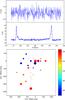 |
Fig. 1 Top panel: total power (I) and stokes V spectra of the OH maser region of OH 12.8-0.9. The V spectrum is shown after removing the residual scaled down of the stokes I. Bottom panel: the OH maser region of OH 12.8-0.9. The offset positions are with respect to the maser reference feature 1. The maser spots are color-coded according to their radial velocity. The size of the spots is scaled logarithmically according to their flux density. |
Properties of the OH maser features of OH 12.8-0.9.
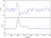 |
Fig. 2 Total intensity (bottom panel) and stokes V (top panel) spectra of the blue shifted OH maser region of OH 12.8-0.9 taken at the position of feature 13. The V spectrum is shown after removing the residual scaled down of the stokes I. |
The properties of the OH maser features identified using the AIPS task SAD are shown in Table 1. Each maser feature consists of several maser spots. On average, we measured a magnetic field of ~−31 μG and ~27 μG for the blue-shifted and red-shifted regions, respectively. The magnetic field measured for the blue- and red-shifted features have opposite signs which may indicate a clear difference between the blue- and red-shifted regions. We found no significant linear polarization for the OH maser features of this source. Additionally, no stokes V signal is apparent in the spectrum shown in Fig. 1, which corresponds to the total V emission from all maser features. However, an individual analysis of the features identified with SAD using the cross-correlation method still produces 3–4σ detections of the magnetic field strength. This is confirmed by the V-spectra, shown in Fig. 2, taken at the location of one of the individual maser feature (feature 13). Now a circular polarization signal is clearly visible.
The spatial distribution of the blue- and red-shifted OH maser spots of OH 12.8-0.9 are plotted in Fig. 1. The spots are color-coded according to their radial velocity. We calculated the average position for the red- and blue-shifted spots. The distribution of the spots implies that the maximum extent of the OH maser region and the offset between the blue- and red-shifted emission are ~500 mas and ~135 mas in the plane of the sky, respectively. The measured offset is slightly higher than the standard deviation in the spread of the red- and blue-shifted maser features (~100 mas), and significantly larger than the positional uncertainty on the individual features (<30 mas). The distance to OH 12.8-0.9 is not accurately known, based on Galactic rotation models it was estimated to be 8 kpc (Baud et al. 1985), but this could be off by a considerable amount. At a distance of 8 kpc, the measured maximum extent of the OH maser region of this source corresponds to 4000 AU. However, the actual extent of the OH maser region could be much larger, since we only detected emission at the blue- and red-shifted peaks and no emission was found close to the stellar velocity (Vlsr = −55 km s-1). The observed distribution does not seem to be explained by the spherically expanding shell model, in which the red- and blue-shifted peaks should be coincident.
3.2. OH maser observations of OH 37.1-0.8
Figure 3 displays the total intensity and stokes V spectra of OH 37.1-0.8. The spectrum shows a double peak structure. The emission is also detected in the circular polarization profile. The red-shifted emission ranges from 73 km s-1 to 78 km s -1. The blue-shifted emission ranges from 95 km s-1 to 103 km s-1. Each of the blue-shifted and red-shifted regions has multiple peaks and is a blend of several lines. In Table 2 we present the maser components that we identified for the OH maser region of this star, using the AIPS task SAD. Each component consists of several maser spots. We did not find significant linear polarization for the OH maser features of this source. On average we measured a magnetic field of ~430 μG and ~230 μG for blue- and red-shifted masers, respectively.
Figure 3 displays the spatial distribution of the OH maser spots of OH 37.1-0.8. We determined the average position for the red- and blue-shifted peaks. The maximum extent of the OH maser region and the offset between the blue- and red-shifted emission are ~200 mas and ~100 mas, respectively. The offset is almost twice higher than the standard deviation in the spread of the red- and blue-shifted maser features (~50 mas). The best estimate for the distance of this source based on galactic rotation model is 8 kpc (Baud et al. 1985). At this distance, the measured maximum extent of the OH maser region of this source is ~1600 AU. This distribution is not consistent with spherically symmetric shell model, since the blue-shifted and red-shifted maser features are not coincident in the plane of the sky.
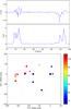 |
Fig. 3 Top panel: total power and the stokes V spectra of the OH maser region of OH 37.1-0.8. The V spectrum is shown after removing the residual scaled down of the stokes I. Bottom panel: the OH maser region of OH 37.1-0.8. The offset positions are with respect to the maser reference feature 7. The maser spots are color-coded according to their radial velocity. The size of the spots is scaled logarithmically according to their flux density. |
Properties of the OH maser features of OH 37.1-0.8.
4. Analysis
4.1. Description of the kinematical reconstruction procedure
The observations of the H2O masers in a number of water-fountain sources revealed that these masers are located in bipolar structures (e.g. Vlemmings et al. 2006; Boboltz & Marvel 2005). Thus the spherically symmetric CSE is modified, for example by carving out polar cavities. In order to understand the geometry of the OH maser region of these sources, we performed a geometrical reconstruction of the masers in three dimensional grids. We did not consider radiative transfer of masers in our analysis. Instead, the velocity coherent path length along the line of sight was determined for maser shells of various geometries and velocity fields. In all cases, we assumed a maximum shell radius of 3 × 1016 cm (~2000 AU), which is typical for OH masers (Chapman & Cohen 1986).
We assumed that the masers are saturated and that the resulting intensity increases linearly rather than exponentially with path-length. Observations indicate that the 1612 MHz respond smoothly and linearly to the change in physical conditions and pump rates, which could indicate that the masers are saturated (Elitzur 1990). Therefore, the saturation assumption enables us to investigate the extent at which the velocity field along the line of sight contributes to the profile and structure of the maser shells, but not the line strengths in detail.
A similar analysis was performed by Bowers (1991), in which they obtained the velocity coherent path length along the line of sight for ellipsoidal shells with various inclinations from the plane of the sky. They also considered different velocity fields, incorporating isotropic velocity, rotation and radial acceleration. We use a similar modeling procedure, but we expand our work to more complex morphologies and velocity fields that may explain the distribution of OH masers in water-fountain sources which show significant deviation from spherically symmetric CSEs. For the basic method we refer to Bowers (1991).
We consider two different possibilities for the distribution of OH masers in water-fountain sources: equatorial distribution (Fig. 4) or biconical outflow (Fig. 5). In the case of equatorial distribution, the OH masers stem from the equatorial region of the circumstellar shell, while the H2O masers are located in a bipolar jet-like outflow. Alternatively, the OH masers may originate in a biconical outflow surrounding the H2O maser jet (Likkel et al. 1992). The spectral profile and emission structure were calculated assuming these two morphologies. Throughout our analysis the opening angle in the case of equatorial distribution is defined as the angle from the equatorial plane. In contrast, for a biconical outflow the opening angle is defined from the polar axis.
We incorporate two different velocity fields: isotropic expansion or azimuthally dependent velocity, either towards the equatorial plane or the polar axis. In the case of isotropic outflow, we assume a constant expansion velocity of 15 km s -1, which is typical for the OH maser in evolved stars (e.g. Sevenster 2002). Since the velocity scales linearly with the extent of the velocity, choosing other values of the expansion velocity does not change the profile shape in our models. In the case where the velocity is enhanced towards the equatorial plane, we use Vexp = a + b × |sin(φ)|. Similarly, if the velocity increases towards the polar axis, we adopt Vexp = a + b × |cos(φ)|. In both cases a + b = 15 km s-1. In all cases φ is the angle from the polar axis.
If the velocity has a latitudinal dependence, we assume an elongated ellipsoid geometry for the maser shell. We define the ellipticity ( ) of the oblate or prolate shells by the velocity ratio between the major and minor axes of the ellipsoid (
 ,
,  ). We present the results for two values of ellipticity (e = 0.7 and e = 0.9), which implies that the velocity of the major axis of the ellipse is twice and four times higher than that for the minor axis of the ellipse. The models in this section have not been adjusted to match the data for a specific object.
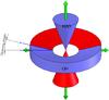 |
Fig. 4 Equatorial distribution of the OH masers surrounding the H2O maser jet in the CSEs of water-fountain sources. The opening angle is shown from the equatorial plane. |
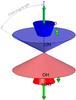 |
Fig. 5 Biconical distribution of the OH masers around the H2O maser jet in the CSEs of water-fountain sources. The opening angle is shown from the polar axis. |
The following plots are presented for each model:
-
1.
normalized intensity profile versus velocity, which indicatesthe path length along the line of sight for each velocity integratedover the sky. We calculated the spectra for inclinations of0°, 15°, 30°, 45°, 60°, 75°, 90° from the plane of the sky. At each inclination, the spectra are presented for 25°, 45°, 65°, 80° opening angles;
-
2.
the offset between the blue-shifted and red-shifted peaks in the plane of the sky. The spatial distribution of the OH maser region of a number of water-fountain sources reveal that the blue-shifted and red-shifted features are separated in the plane of the sky. For the cases where the spectrum shows the typical double peak profile, we calculated the position of the blue-shifted and red-shifted peaks and measured the offset. For more complex spectra where the spectra show inner peaks it becomes more complicated as the position of the inner peaks and outer peaks are different. Therefore, we measured the position of the outer peaks for the blue-shifted and red-shifted emission and determined the offset value. For example, Fig. 6 shows the distribution of the blue-shifted and red-shifted peaks in the case where masers are confined within 30° from the equatorial plane with an inclination of 40° from the sky plane, which shows that the OH masers are reversed in the plane of the sky compared to those of the bipolar outflow. Similarly, for all cases we determined the separation between the blue shifted and red shifted regions. The negative sign for the offset values implies that the masers are located in the opposite direction with respect to the fast bipolar H2O maser outflow.
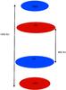 |
Fig. 6 The offset between the blue-shifted and red-shifted peaks of maser emission calculated from the models. The OH masers are confined within 30° from the equatorial plane with an inclination of 40° from the plane of the sky. The models show that the OH masers are reversed in the plane of the sky compared to those of the bipolar H2O maser outflow. |
We consider different scenarios, which are intended as a guide for analysis of the OH masers in water-fountain sources. The plots presented are particularly useful for comparison with the observed parameters of spectral structure and spatial distribution in these objects. Figures 7 and 8 show the results for the cases of equatorial and biconical distribution of the masers, where the expansion velocity is constant in all directions. For the other cases where the velocity has latitudinal dependence we present the result of our modeling calculations in Figs. 6–19.
A1: Equatorial distribution, Vexp = const.
This case describes the situation that the OH masers remain active in the equatorial plane, while H2O masers originate in a high velocity outflow in the polar region. The outflow velocity is constant in all directions. The OH masers in this scenario would have a slower expansion velocity with respect to the fast outflow in the polar region.
Figure 7 displays the results for this case. The spectra show double peak structure for inclinations below 45° from the plane of the sky. For 60° and 75° inclinations, the spectra display inner peaks for opening angles smaller than 45°. At 90°, the spectra again show double peaks.
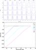 |
Fig. 7 Model calculations for the case of isotropic outflow of 15 km s-1 with equatorial distribution. The top panel shows the spectra calculated for inclinations of 0°, 15°, 30°, 45°, 60°, 75°, 90° from the plane of the sky. For each inclination the spectra are shown for 25°, 45°, 65° and 80° opening angle from the equatorial plane. The bottom panel displays the offset between the blue shifted and red shifted regions in the plane of the sky. The negative sign indicates that the masers are reversed in the plane of the sky compared to those located in a narrow region in the polar axis. |
The diagram at the bottom shows the offset between the blue-shifted and red-shifted regions versus opening angle from the equatorial plane. Each line shows the offset at a specific inclination. For 0°, 15° and 90° inclination angle from the plane of the sky, the separation is zero and the blue-shifted and red-shifted emission coincide in the plane of the sky. For other inclinations the masers are reversed in the sky plane. The offset is highest at small opening angles and as expected approaches 0 for large opening angles in the equatorial region. The highest offset is ~3000 AU.
A2: Equatorial distribution, Vexp = a + b × |sin(φ)|
Similar to case A1, we assume equatorial distribution for the masers. But we adopt a latitudinal dependent velocity of Vexp = a + b × |sin(φ)|, where the velocity is highest in the equatorial plane and decreases towards the polar region. The shell geometry is elongated towards the equatorial plane. This case potentially describes the situation where the masers are affected by a binary companion in the equatorial region of the CSE.
We calculated the spectra and map structure for e = 0.7 and e = 0.9. The results of this case are shown in Figs. 9 and 10. Comparison of the spectra obtained for this scenario and those for the case A1, shows that the shape of the spectra remains similar at inclinations below 60°, where the spectra show double peaks. Above 60° inclination the inner peaks occur, which dominate the emission at the edges of the spectrum for the case of e = 0.9.
Again, the second figure displays the offset value between the blue-shifted and red-shifted peaks. At 0° and 90° inclinations from the plane of the sky, the separation is zero. For other inclinations the masers are reversed and the offset is in the range 400–2500 AU and 400–2500 AU for the cases of e = 0.7 and e = 0.9, respectively.
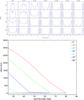 |
Fig. 8 Model calculations for the case of biconical outflow with constant expansion velocity of 15 km s-1. |
A3: Equatorial distribution,Vexp = a + b × |cos(φ)|
In this case we assumed equatorial distribution for the masers but the shell geometry is considered to be elongated towards the polar axis. The velocity field is latitudinally dependent (Vexp = a + b × |cos(φ)|), which implies that the velocity increases towards the polar region.
We calculated the models for e = 0.7 and e = 0.9, the results of which are shown in Figs. 11 and 12. The spectra show significant differences compared to the case A1, where the velocity is constant in all directions. For all inclinations the spectra show inner peaks, which are even higher than the emission at the edges of the spectrum for opening angles smaller than 45°.
The bottom figure shows the separation between the blue shifted and red shifted regions. For 0° and 90° inclination from the plane of the sky, the offset between the blue shifted and red shifted regions is zero. At 45°, 60° and 75° inclinations the masers are reversed when the opening angle is smaller than 45°, 60° and 75° from the equatorial plane, respectively. The maximum offset value is ~1500 AU and ~800 AU for the cases of e = 0.7 and e = 0.9, respectively.
Biconical distribution, Vexp = const.
A biconical distribution is another possibility for the distribution of OH masers in water-fountain sources (Likkel et al. 1992; Sahai et al. 1999). In this case, the OH masers are located in a biconical outflow surrounding the H2O maser jet, but at lower latitudes (Fig. 5) with a constant expansion velocity of 15 km s-1.
Figure 8 displays the results for this case. The spectra show double peak structures generally. However, at inclinations of 0°, 15° and 30° there are strong inner peaks for small opening angles (i ≤ 45).
For 0° and 90° inclination angle from the sky plane the offset between the blue-shifted and red-shifted peaks is zero. In contrast to case A1, the masers are not reversed in the plane of the sky. The maximum offset value is 3000 AU.
B2: biconical distribution, Vexp = a + b × |sin(φ)|
In this scenario, the masers are distributed in a biconical outflow and the expansion velocity increases azimuthally towards the equatorial region. This case describes the situation where the masers are affected by a binary companion in the equatorial region, while they are still entrained by the fast collimated outflow in the polar region.
We calculated the models for e = 0.7 and e = 0.9. The results of this case are shown in Figs. 13 and 14. Comparison of the spectra obtained for this case and those for the case B1 show significant differences in the profile structure for inclinations above 45°, where most of the spectra show inner peak emission.
The bottom figure shows the offset between the blue-shifted and red-shifted emission. The masers are reversed for large inclinations from the plane of the sky, in particular at 45°, 60° and 75°. The maximum offset value is ~1500 AU and ~800 AU for e = 0.7 and e = 0.9 respectively.
B3: biconical distribution, Vexp = a + b × |cos(φ)|
In this case, the masers are distributed in a biconical outflow and the velocity has latitudinal dependence towards the polar axis. Figures 15 and 16 show the results for e = 0.9 e = 0.9 cases.
For 45° to 90° inclination angle from the plane of the sky, the spectra show double peak profiles, however for 0° to 30° inclinations the spectra show inner peaks. The offset between the blue shifted and red shifted regions is higher for smaller opening angles and approaches zero for higher opening angles. The maximum offset value is ~2500 AU and ~1600 AU for e = 0.7 and e = 0.9 respectively.
4.2. Application to individual sources
4.2.1. W43A
W43A is a unique water-fountain source because it exhibits OH (1612, 1665 and 1667 MHz), H2O and SiO masers (A10; Nyman et al. 1998; Imai et al. 2002). The spectra of the OH and H2O masers of this object exhibit double peak profiles. The H2O maser velocity range (~180 km s-1) is much higher than that for the OH masers (~13 km s-1), which makes this the archetype water-fountain source (Imai et al. 2002; Likkel et al. 1992).
High resolution interferometric observations of the H2O maser region of W43A revealed a highly collimated and precessing jet. The H2O masers are found in two opposing clusters separated by ~1700 AU at a distance of 2.6 kpc (Diamond et al. 1985). The H2O maser jet has an outflow velocity of ~145 km s-1 with 39° inclination from the plane of the sky (Imai et al. 2002). The SiO masers of this source are thought to occur in a shock at the interface between the fast collimating jet and the slow biconical outflow (Imai et al. 2005). The spatial distribution of the OH maser region of W43A revealed that the OH masers are located inside the H2O maser region. The OH masers are found in two opposing clusters separated by ~650 AU. The red-shifted and blue-shifted OH masers are reversed in the plane of the sky with respect to those of H2O masers (A10).
The fact that the blue and red-shifted OH maser features are not positionally coincident in the plane of the sky, is not consistent with an isotropically expanding shell model. Additionally, the bipolar structure of the H2O and SiO maser regions is another piece evidence that these masers are located in aspherical shells.
The expansion velocity of the OH maser region of W43A is ~18 km s-1 (A10). This seems to imply that the OH maser region is not affected by the fast post-AGB wind. We considered the two scenarios of either an equatorial distribution or a biconical outflow, as explained in Sect. 4.1 and compared the spectral profile and the OH masers spatial distribution with the model calculations. The same inclination (39°) as that of the collimated H2O maser jet was adopted for the OH maser region (Imai et al. 2002).
If the masers are distributed in the equatorial plane of the circumstellar shell with a constant expansion velocity in all directions, then our calculations show that the masers are reversed in the plane of the sky and the spectra would show double peak structures for all opening angles in the equatorial region (Fig. 7). For an opening angle of ~35°, the offset corresponds to the observed value of ~650 AU. If the velocity is azimuthally enhanced towards the equatorial plane, the spectra would show double peak profiles in all opening angles (Figs. 9 and 10). The models show that the masers are reversed in the plane of the sky, and the offset is in the range 400 AU to 700 AU for all opening angles in the equatorial plane. Therefore, this case may also describe the distribution of the OH masers of W43A.
On the other hand if the velocity has latitudinal dependence enhanced towards the polar axis, the spectra show inner peaks (Fig. 12). These profile shapes are not consistent with the OH maser profile of W43A. Therefore, this scenario is unlikely for the OH maser region of W43A.
Alternatively, we considered biconical distribution of the OH maser region of W43A. If the velocity is isotropic or azimuthally enhanced towards the polar axis, the masers are not reversed in the plane of the sky (Figs. 8 and 16), which is not consistent with the OH maser morphology of W43A. However, if the velocity is azimuthally enhanced towards the equatorial region, the spectra show double peak profiles at opening angles larger than 70°, for which the separation between the blue shifted and red shifted regions is ~650 AU (Fig. 14). Therefore, this scenario may also explain the OH maser morphology of W43A. However, for such large opening angles we are approaching an oblate distribution with enhanced outflow in the equatorial region. Thus, in either case, the reconstruction of the OH maser region of W43A suggests a predominantly equatorial distribution.
4.2.2. OH 12.8-0.9
OH 12.8-0.9 is a water-fountain candidate. This source was first reported by Baud et al. (1979) as a type II OH/IR star on the basis of its double peak 1612 MHz OH maser profile. The source IRAS 18316-1816 is identified as the IR counterpart to this source. The H2O masers of OH 12.8-0.9 were first discovered by Engels et al. (1986). They also found that the OH masers of this object lie inside the H2O maser velocity range, which is not typical for OH/IR stars. VLBI H2O maser observations of this object revealed that the masers are located in two opposing clusters at the tips of a bipolar jet-like structure oriented north-south (Boboltz & Marvel 2005). The blue-shifted and red-shifted H2O masers are found in arc-shape structures separated by ~110 mas in the plane of the sky.
Multi-epoch VLBA observations revealed a 3D outflow velocity of 58 km s-1 for the H2O maser jet with 24° inclination from the plane of the sky (Boboltz & Marvel 2007). Comparison of the spatial morphology of the OH masers (Fig. 1) and the H2O masers reveal that the OH masers are located outside the H2O maser jet. The maximum extent of the OH maser region is ~500 mas, which is much larger than that for H2O masers (~110 mas). This is in contrast to Boboltz & Marvel (2005) expectation that the OH masers should be located inside the H2O maser jet. Since this object is characterized as a high mass-loss source it is possible that this source is still in the AGB phase and that the jet has recently turned on in this source (Deacon et al. 2007).
We compared the observational parameters of the profile shape and spatial distribution (Fig. 1) with our model calculations. The OH maser spectrum of this source shows a double peak structure. Our observations show that the separation between the blue shifted and red shifted OH maser region of this source is ~135 mas (Fig. 1). Assuming a distance of 8 kpc for this source, the offset corresponds to 1080 AU. Unlike W43A, the blue-shifted and red-shifted OH masers are not reversed in the plane of the sky compared to those of H2O masers.
The equatorial distribution of the masers is unlikely. Our models show that the masers are reversed in the plane of the sky at 24° in the case of isotropic outflow and latitudinal dependent velocity enhanced towards the equatorial region (Figs. 7, 10). However, in the case where the velocity azimuthally increases towards the polar region, the masers are not reversed in the plane of the sky, but the spectral shapes in this case are quadruply peaked (Fig. 12), which is not consistent with the observed spectrum of this source.
If the masers are located in a biconical outflow with isotropic expansion velocity or azimuthal dependent velocity towards the polar axis, our results show that at opening angles of ≥ 65°, the spectra show double peak profiles (Figs. 8 and 16). However, the offset between the blue shifted and red shifted regions is smaller than 1000 AU. This implies that either the distance of 8 kpc is not accurate for this source or the assumption of maximum shell radius of 2000 AU is not correct. In the case of a biconical distribution where the velocity enhances towards the equatorial region (Fig. 14), at opening angles above 65° the profile shape is double peaked, however the offset approaches zero at these large opening angles, which is not consistent with the observed spatial distribution of the OH maser region of this source. Therefore, a biconical outflow with isotropic expansion velocity or azimuthal dependent velocity towards the polar axis may explain the OH maser morphology of this source. However, we do not consider other effects (e.g. anisotropic pumping, etc.), that may produce the observed asymmetry of the OH maser region of this source.
4.2.3. OH 37.1-0.8
The H2O masers of this source were first discovered by Engels et al. (1986) and the OH masers were first detected by Winnberg et al. (1975). The H2O maser velocity range of this source (63–114 km s-1; Engels 2002) is higher than that for OH masers (73–103 km s-1), which establishes the water-fountain nature of this source.
The spatial distribution of the OH maser of this source shows that these masers are located in aspherical shell. The separation between the two corresponds to ~100 mas (Fig. 3). Since no high resolution map of the H2O masers of this source is available, the spatial distribution of the OH maser features with respect to H2O masers is not clear in this source. Additionally, we do not have information on the orientation of the jet from the plane of the sky. Therefore, we can not easily distinguish between the equatorial or biconical outflow scenarios for the OH maser region of this source.
However, the OH maser spectrum of this source shows double peaks, but each peak is a blend of several maser lines. This could raise two possibilities. These peaks could originate from several maser spots with different velocities. Alternatively, geometric effects can produce this profile structure. Our calculations show that multiple peaks in the spectra may form in both biconical outflow and equatorial distribution; for example Figs. 12, 14.
5. Discussions
Our observations reveal that the OH maser region of the three water-fountain sources studied in this work show signs of non-spherical expansion. This morphology can not be explained by the standard spherically expanding shell model for the OH maser shells in evolved stars. The dynamical ages of the H2O maser jets of W43A & OH 12.8-0.9 are 90 and 50 yr, respectively (Boboltz & Marvel 2007; Imai et al. 2005). We measured a shell size of > 1600 AU and the expansion velocity of < 15 km s-1 for the OH masers. This implies the dynamical time scale of ~506 yr. This indicates that the OH maser region is significantly older compared to the H2O maser jet. Therefore, the collimating agent was likely already at work before the H2O maser jet was launched. No H2O maser image of OH 37.1-0.8 is available. Therefore we can not confirm whether the jet is older that the OH maser shell in this star. Alternatively, the observed asymmetry may not reflect an actual asymmetry in the distribution, but rather other effects such as anisotropic pumping.
Recent observations have shown that magnetic fields could have an important role in collimating the H2O maser jets in water-fountain sources. Vlemmings et al. (2006) show that the H2O maser jet of W43A is magnetically collimated. The bipolar H2O masers, can be explained by the dynamo-driven magnetic field. Blackman et al. (2001) showed that a single star model can produce magnetic driven dynamo in the AGB phase. However, since magnetic field drains rotational energy, it needs to be reseeded. A binary companion can maintain the differential rotation required during the lifetime of the AGB phase. In the presence of a binary companion, the in-spiral of the companion into the envelope produces rotational energy needed for the generation of the magnetic field (Nordhaus & Blackman 2006).
Magnetic fields could also have an important role on the non-spherical shape of the OH masers in water-fountain sources. From our MERLIN observations, we measured a magnetic field of ~430 μG and ~230 μG for blue shifted and red shifted masers of OH 37.1-0.8, respectively. These values are approximately an order of magnitude larger than those measured for the OH maser features of OH 12.8-0.9 (~27 μG and ~–31 μG for the blue-shifted and red-shifted regions, respectively). Previous MERLIN observations of the OH masers of W43A also revealed a field strength of 100 μG (A10), which indicates that a large scale magnetic field is present in the circumstellar environment of this object. A10 discussed several non-Zeeman effects which could produce the observed circular polarization. These effects include observational and instrumental effects. However, they did not find any effects which could falsely be attributed to the Zeeman splitting. This implies that the circular polarization observed in the OH masers originates from the Zeeman splitting.
The fact that the field strength measured for OH 37.1-0.8 is almost an order of magnitude larger than that for OH 12.8-0.9 could imply that the OH maser region of OH 37.1-0.8 is located at a smaller distance to the central star than that of OH 12.8-0.9. As shown in Figs. 1 and 3, the maximum extent of the OH maser region of OH37.1-0.8 is ~200 mas, which is ~2.5 times smaller than the OH maser region of OH 12.8-0.9 (~500 mas). The magnetic field strength changes as a function of distance from the central star (Vlemmings et al. 2005, Fig. 6). The dipole field has r-3 dependence and the solar type field has r-2 dependence, where r is the distance from the central star. The distance to these stars is poorly known. However, considering the maximum extent of the OH maser region of these objects, it could be due to the difference in size of the OH maser shell that we measure different field strengths. Therefore, depending on the magnetic field morphology, the field strength in the OH maser region of OH 37.1-0.8 could be higher than that of OH 12.8-0.9 by up to an order of magnitude.
We performed geometrical reconstruction in order to clarify the morphology of the OH maser region in water-fountain sources. We have studied the effects of many different parameters including the spectral shape, velocity field and the equatorial or biconical morphology. Our analyses show that the OH maser spots of W43A are likely located in the equatorial region of the circumstellar shell, while in OH 12.8-0.9 the OH masers are likely found in a biconical outflow surrounding the H2O maser jet. The equatorial enhancement could be produced by the presence of a binary companion close to the CSE via common envelope (CE) evolution (Nordhaus & Blackman 2006). Under certain conditions the Roche lobe overflow, in a binary system may result in both companions immersed in a CE (Paczynski 1976). Numerical simulations showed that a binary induced equatorial outflow is confined to opening angles of 20°–30° (Terman & Taam 1996).
Although the binary companion could explain the equatorial enhancement, at the same time it may destroy the maser action. Schwarz et al. (1995) performed statistical analysis for a limited sample of symbiotics, most of them containing Mira variables as primaries. Their analysis showed that for very wide systems (R ≥ 50 AU), all masers (OH, H2O and SiO) can operate. At intermediate orbits (10 AU ≤ R ≤ 50 AU) SiO and H2O but not OH masers can survive. For much closer orbits (R ≤ 10 AU) no maser operates. The absence of masers in the close binary systems may be explained by the tidal effects from the secondary on the maser regions. Therefore, in water-fountain sources which show OH and sometimes SiO maser activity, the orbital separation is wide enough, that the masers are not affected by the companion (Deacon et al. 2007). Alternatively, the companion may already be swept up by the primary and does not influence the maser regions which occur at much larger distances from the central star.
6. Conclusions
The observations show that the OH masers in water-fountain sources are located in aspherical shells. We performed geometrical reconstruction in order to understand the morphology of the OH masers. The comparison between the observations and models show that the OH masers of W43A are likely located in the equatorial region of the circumstellar shell, while in OH 12.8-0.9 the OH masers stem from a biconical outflow surrounding the H2O maser jet. We measured significant magnetic fields for the OH maser region of OH 12.8-0.9 and OH 37.1-0.8. This shows the possible role of the magnetic field in shaping the CSE of these stars.
Online material
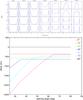 |
Fig. 9 As in Fig. 7, model calculations for the oblate ellipsoid e = 0.7 with equatorial distribution, where the velocity in the equatorial region is twice that in the polar axis. |
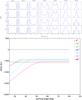 |
Fig. 10 As in Fig. 7, model calculations for the oblate ellipsoid (e = 0.9) with equatorial distribution,where the velocity in the equatorial region is four times higher than that in the polar axis. |
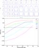 |
Fig. 11 As in Fig. 7, model calculations for the prolate ellipsoid (e = 0.7) with equatorial distribution, where the velocity in the polar axis is twice than that in the equatorial plane. |
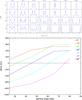 |
Fig. 12 As in Fig. 7, model calculations for the prolate ellipsoid (e = 0.9) with equatorial distribution, where the velocity in the polar axis is four times higher than that in the equatorial plane. |
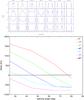 |
Fig. 13 As in Fig. 8, model calculations for the oblate ellipsoid (e = 0.7) with biconical distribution, where the outflow velocity increases towards the equatorial plane. |
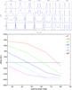 |
Fig. 14 As in Fig. 8, model calculations for the oblate ellipsoid (e = 0.9) with biconical distribution, where the outflow velocity increases towards the equatorial plane. |
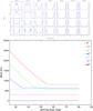 |
Fig. 15 As in Fig. 8, model calculations for the prolate ellipsoid (e = 0.7) with biconical distribution, where the outflow velocity increases towards the polar region. |
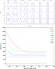 |
Fig. 16 As in Fig. 8, model calculations for the prolate ellipsoid (e = 0.9) with biconical distribution, where the outflow velocity increases towards the polar region. |
Acknowledgments
This research was supported by the ESTRELA fellowship, the EU Framework 6 Marie Curie Early Stage Training program under contract number MEST-CT-2005-19669. We acknowledge MERLIN staff for their help in the observation and reducing the data. We thank Anita Richards for helping us with the initial data processing at Jodrell Bank. W.V. acknowledges support by the Deutsche Forschungsgemeinschaft through the Emmy Noether Research grant VL 61/3-1.
References
- Amiri, N., Vlemmings, W., & van Langevelde, H. J. 2010, A&A, 509, A26 [NASA ADS] [CrossRef] [EDP Sciences] [Google Scholar]
- Baud, B., Habing, H. J., Matthews, H. E., & Winnberg, A. 1979, A&AS, 36, 193 [NASA ADS] [Google Scholar]
- Baud, B., Sargent, A. I., Werner, M. W., & Bentley, A. F. 1985, ApJ, 292, 628 [NASA ADS] [CrossRef] [Google Scholar]
- Blackman, E. G., Frank, A., Markiel, J. A., Thomas, J. H., & Van Horn, H. M. 2001, Nature, 409, 485 [NASA ADS] [CrossRef] [PubMed] [Google Scholar]
- Boboltz, D. A., & Marvel, K. B. 2005, ApJ, 627, L45 [NASA ADS] [CrossRef] [Google Scholar]
- Boboltz, D. A., & Marvel, K. B. 2007, ApJ, 665, 680 [NASA ADS] [CrossRef] [Google Scholar]
- Bowers, P. F. 1991, ApJS, 76, 1099 [NASA ADS] [CrossRef] [Google Scholar]
- Chapman, J. M., & Cohen, R. J. 1986, MNRAS, 220, 513 [NASA ADS] [Google Scholar]
- Claussen, M., Sahai, R., & Morris, M. 2004, in Asymmetrical Planetary Nebulae III: Winds, Structure and the Thunderbird, ed. M. Meixner, J. H. Kastner, B. Balick, & N. Soker, ASP Conf. Ser., 313, 331 [Google Scholar]
- Deacon, R. M., Chapman, J. M., Green, A. J., & Sevenster, M. N. 2007, ApJ, 658, 1096 [NASA ADS] [CrossRef] [Google Scholar]
- Diamond, P. J., Norris, R. P., Rowland, P. R., Booth, R. S., & Nyman, L. 1985, MNRAS, 212, 1 [NASA ADS] [CrossRef] [Google Scholar]
- Elitzur, M. 1990, ApJ, 363, 628 [NASA ADS] [CrossRef] [Google Scholar]
- Engels, D. 2002, A&A, 388, 252 [NASA ADS] [CrossRef] [EDP Sciences] [Google Scholar]
- Engels, D., Schmid-Burgk, J., & Walmsley, C. M. 1986, A&A, 167, 129 [NASA ADS] [Google Scholar]
- García-Segura, G., López, J. A., & Franco, J. 2005, ApJ, 618, 919 [NASA ADS] [CrossRef] [Google Scholar]
- Habing, H. J. 1996, A&ARv, 7, 97 [NASA ADS] [CrossRef] [Google Scholar]
- Imai, H., Obara, K., Diamond, P. J., Omodaka, T., & Sasao, T. 2002, Nature, 417, 829 [NASA ADS] [CrossRef] [PubMed] [Google Scholar]
- Imai, H., Nakashima, J., Diamond, P. J., Miyazaki, A., & Deguchi, S. 2005, ApJ, 622, L125 [NASA ADS] [CrossRef] [Google Scholar]
- Likkel, L., Morris, M., & Maddalena, R. J. 1992, A&A, 256, 581 [NASA ADS] [Google Scholar]
- Manchado, A., Villaver, E., Stanghellini, L., & Guerrero, M. A. 2000, in Asymmetrical Planetary Nebulae II: From Origins to Microstructures, ed. J. H. Kastner, N. Soker, & S. Rappaport, ASP Conf. Ser., 199, 17 [Google Scholar]
- Modjaz, M., Moran, J. M., Kondratko, P. T., & Greenhill, L. J. 2005, ApJ, 626, 104 [NASA ADS] [CrossRef] [Google Scholar]
- Morris, M. R., Sahai, R., & Claussen, M. 2003, in Rev. Mex. Astron. Astrof. Conf. Ser., ed. J. Arthur, & W. J. Henney, 15, 20 [Google Scholar]
- Nordhaus, J., & Blackman, E. G. 2006, MNRAS, 370, 2004 [NASA ADS] [CrossRef] [Google Scholar]
- Nordhaus, J., Blackman, E. G., & Frank, A. 2007, MNRAS, 376, 599 [NASA ADS] [CrossRef] [Google Scholar]
- Nyman, L., Hall, P. J., & Olofsson, H. 1998, A&AS, 127, 185 [NASA ADS] [CrossRef] [EDP Sciences] [Google Scholar]
- Paczynski, B. 1976, in Structure and Evolution of Close Binary Systems, ed. P. Eggleton, S. Mitton, & J. Whelan, IAU Symp., 73, 75 [Google Scholar]
- Reid, M. J., & Moran, J. M. 1981, ARA&A, 19, 231 [NASA ADS] [CrossRef] [Google Scholar]
- Sahai, R., & Trauger, J. T. 1998, AJ, 116, 1357 [NASA ADS] [CrossRef] [Google Scholar]
- Sahai, R., te Lintel Hekkert, P., Morris, M., Zijlstra, A., & Likkel, L. 1999, ApJ, 514, L115 [NASA ADS] [CrossRef] [Google Scholar]
- Schwarz, H. E., Nyman, L., Seaquist, E. R., & Ivison, R. J. 1995, A&A, 303, 833 [NASA ADS] [Google Scholar]
- Sevenster, M. N. 2002, AJ, 123, 2772 [NASA ADS] [CrossRef] [Google Scholar]
- Terman, J. L., & Taam, R. E. 1996, ApJ, 458, 692 [NASA ADS] [CrossRef] [Google Scholar]
- Vlemmings, W. H. T., van Langevelde, H. J., & Diamond, P. J. 2005, A&A, 434, 1029 [NASA ADS] [CrossRef] [EDP Sciences] [Google Scholar]
- Vlemmings, W. H. T., Diamond, P. J., & Imai, H. 2006, Nature, 440, 58 [NASA ADS] [CrossRef] [PubMed] [Google Scholar]
- Walsh, A. J., Breen, S. L., Bains, I., & Vlemmings, W. H. T. 2009, MNRAS, 394, L70 [NASA ADS] [Google Scholar]
- Winnberg, A., Nguyen-Quang-Rieu,Johansson, L. E. B., & Goss, W. M. 1975, A&A, 38, 145 [NASA ADS] [Google Scholar]
All Tables
All Figures
|
Fig. 1 Top panel: total power (I) and stokes V spectra of the OH maser region of OH 12.8-0.9. The V spectrum is shown after removing the residual scaled down of the stokes I. Bottom panel: the OH maser region of OH 12.8-0.9. The offset positions are with respect to the maser reference feature 1. The maser spots are color-coded according to their radial velocity. The size of the spots is scaled logarithmically according to their flux density. |
| In the text | |
|
Fig. 2 Total intensity (bottom panel) and stokes V (top panel) spectra of the blue shifted OH maser region of OH 12.8-0.9 taken at the position of feature 13. The V spectrum is shown after removing the residual scaled down of the stokes I. |
| In the text | |
|
Fig. 3 Top panel: total power and the stokes V spectra of the OH maser region of OH 37.1-0.8. The V spectrum is shown after removing the residual scaled down of the stokes I. Bottom panel: the OH maser region of OH 37.1-0.8. The offset positions are with respect to the maser reference feature 7. The maser spots are color-coded according to their radial velocity. The size of the spots is scaled logarithmically according to their flux density. |
| In the text | |
|
Fig. 4 Equatorial distribution of the OH masers surrounding the H2O maser jet in the CSEs of water-fountain sources. The opening angle is shown from the equatorial plane. |
| In the text | |
|
Fig. 5 Biconical distribution of the OH masers around the H2O maser jet in the CSEs of water-fountain sources. The opening angle is shown from the polar axis. |
| In the text | |
|
Fig. 6 The offset between the blue-shifted and red-shifted peaks of maser emission calculated from the models. The OH masers are confined within 30° from the equatorial plane with an inclination of 40° from the plane of the sky. The models show that the OH masers are reversed in the plane of the sky compared to those of the bipolar H2O maser outflow. |
| In the text | |
|
Fig. 7 Model calculations for the case of isotropic outflow of 15 km s-1 with equatorial distribution. The top panel shows the spectra calculated for inclinations of 0°, 15°, 30°, 45°, 60°, 75°, 90° from the plane of the sky. For each inclination the spectra are shown for 25°, 45°, 65° and 80° opening angle from the equatorial plane. The bottom panel displays the offset between the blue shifted and red shifted regions in the plane of the sky. The negative sign indicates that the masers are reversed in the plane of the sky compared to those located in a narrow region in the polar axis. |
| In the text | |
|
Fig. 8 Model calculations for the case of biconical outflow with constant expansion velocity of 15 km s-1. |
| In the text | |
|
Fig. 9 As in Fig. 7, model calculations for the oblate ellipsoid e = 0.7 with equatorial distribution, where the velocity in the equatorial region is twice that in the polar axis. |
| In the text | |
|
Fig. 10 As in Fig. 7, model calculations for the oblate ellipsoid (e = 0.9) with equatorial distribution,where the velocity in the equatorial region is four times higher than that in the polar axis. |
| In the text | |
|
Fig. 11 As in Fig. 7, model calculations for the prolate ellipsoid (e = 0.7) with equatorial distribution, where the velocity in the polar axis is twice than that in the equatorial plane. |
| In the text | |
|
Fig. 12 As in Fig. 7, model calculations for the prolate ellipsoid (e = 0.9) with equatorial distribution, where the velocity in the polar axis is four times higher than that in the equatorial plane. |
| In the text | |
|
Fig. 13 As in Fig. 8, model calculations for the oblate ellipsoid (e = 0.7) with biconical distribution, where the outflow velocity increases towards the equatorial plane. |
| In the text | |
|
Fig. 14 As in Fig. 8, model calculations for the oblate ellipsoid (e = 0.9) with biconical distribution, where the outflow velocity increases towards the equatorial plane. |
| In the text | |
|
Fig. 15 As in Fig. 8, model calculations for the prolate ellipsoid (e = 0.7) with biconical distribution, where the outflow velocity increases towards the polar region. |
| In the text | |
|
Fig. 16 As in Fig. 8, model calculations for the prolate ellipsoid (e = 0.9) with biconical distribution, where the outflow velocity increases towards the polar region. |
| In the text | |
Current usage metrics show cumulative count of Article Views (full-text article views including HTML views, PDF and ePub downloads, according to the available data) and Abstracts Views on Vision4Press platform.
Data correspond to usage on the plateform after 2015. The current usage metrics is available 48-96 hours after online publication and is updated daily on week days.
Initial download of the metrics may take a while.