| Issue |
A&A
Volume 532, August 2011
|
|
|---|---|---|
| Article Number | A57 | |
| Number of page(s) | 26 | |
| Section | Cosmology (including clusters of galaxies) | |
| DOI | https://doi.org/10.1051/0004-6361/201016348 | |
| Published online | 22 July 2011 | |
Mass, light and colour of the cosmic web in the supercluster SCL2243-0935 (z = 0.447)⋆,⋆⋆
1
Argelander-Institut für Astronomie, Universität Bonn, Auf dem Hügel 71, 53121 Bonn, Germany
e-mail: This email address is being protected from spambots. You need JavaScript enabled to view it.
2
Isaac Newton Group of Telescopes, Calle Alvarez Abreu 70, 38700 Santa Cruz de La Palma, Spain
3
Leiden Observatory, Leiden University, Niels Bohrweg 2, 2333 Leiden, The Netherlands
4
Department of Physics and Astronomy, 6224 Agricultural Road, University of British Columbia, Vancouver, Canada
Received: 17 December 2010
Accepted: 31 March 2011
Abstract
Aims. In archival 2.2 m MPG-ESO/WFI data we discovered several mass peaks through weak gravitational lensing, forming a possible supercluster at redshift 0.45. Through wide-field imaging and spectroscopy we aim to identify the supercluster centre, confirm individual member clusters, and detect possible connecting filaments.
Methods. Through multi-colour imaging with CFHT/Megaprime and INT/WFC we identify a population of early-type galaxies and use it to trace the supercluster network. EMMI/NTT multi-object spectroscopy is used to verify the initial shear-selected cluster candidates. We use weak gravitational lensing to obtain mass estimates for the supercluster centre and the filaments.
Results. We identified the centre of the SCL2243-0935 supercluster, MACS J2243-0935, which was found independently by Ebeling et al. (2001, 2010). We found 13 more clusters or overdensities embedded in a large filamentary network. Spectroscopic confirmation for about half of them is still pending. Three  Mpc filaments are detected, and we estimate the global size of SCL2243 to be
  Mpc, making it one of the largest superclusters known at intermediate redshifts. Weak lensing yields
  Mpc and M200 = (1.54 ± 0.29) × 1015 M⊙ for MACS J2243 with M/L = 428 ± 82, very similar to results from size-richness cluster scaling relations. Integrating the weak lensing surface mass density over the supercluster network (defined by increased i-band luminosity or g − i colours), we find (1.53 ± 1.01) × 1015 M⊙ and M/L = 305 ± 201 for the three main filaments, consistant with theoretical predictions. The filaments’ projected dimensionless surface mass density κ varies between 0.007 − 0.012, corresponding to ρ/ρcrit = 10 − 100 depending on location and de-projection. The greatly varying density of the cosmic web is also reflected in the mean colour of galaxies, e.g. ⟨ g − i ⟩ = 2.27 mag for the supercluster centre and 1.80 mag for the filaments.
Conclusions. SCL2243 is significantly larger and much more richly structured than other known superclusters such as A901/902 or MS0302 studied with weak lensing before. It is a text-book supercluster with little contamination along the line of sight, making it a perfect sandbox for testing new techniques probing the cosmic web.
Key words: galaxies: clusters: individual: SCL2243-0935 / gravitational lensing: weak / large-scale structure of Universe / dark matter / cosmology: observations
This work is based on observations obtained with MegaPrime/MegaCam, a joint project of CFHT and CEA/DAPNIA, at the Canada-France-Hawaii Telescope (CFHT) which is operated by the National Research Council (NRC) of Canada, the Institut National des Sciences de l’Univers of the Centre National de la Recherche Scientifique (CNRS) of France, and the University of Hawaii (programme ID: 2008BO01); based on observations made with ESO Telescopes at the La Silla and Paranal Observatories, Chile (ESO Programmes 165.S-0187 and 079.A-0063); based on observations made with the 2.5 m Isaac Newton Telescope operated on the island of La Palma by the Isaac Newton Group in the Spanish Observatorio del Roque de los Muchachos of the Instituto de Astrofisica de Canarias (programme ID 2008B/C11 and 2009B/C1).
Appendices are available in electronic form at http://www.aanda.org
© ESO, 2011
1. Introduction
Superclusters of galaxies mark the largest and most massive structures known in the Universe, tracing the transition from the linear to the non-linear regime in the evolution of the density contrast. Being non-virialised, they usually come in the form of long filaments (Bond et al. 1996), and it is not a priori clear that they form gravitationally bound systems (Gramann & Suhhonenko 2002). The evolution of a supercluster’s global structure is driven by gravitation only, as hydrodynamic or intergalactic processes become important on cluster scales and below. Beyond a certain extent superclusters are also very susceptible to (accelerated) cosmic expansion. Araya-Melo et al. (2009) have shown that in the ΛCDM paradigm superclusters can withstand expansion and will eventually collapse, provided that their average density inside a spherical shell exceeds 2.36 ρcrit.
Known superclusters at redshifts 0.2 < z < 1.0 with at least three member clusters.
The morphologies and appearances of superclusters are quite diverse. Einasto et al. (2007a) divided their sample of 543 superclusters selected from the 2dF Galaxy Redshift Survey (Colless et al. 2001) into four richness classes, parametrised by the number of peaks in the smoothed and luminosity-weighted density field. Poor superclusters contain 1−2 such clusters, whereas richer systems have several large compact cores of high density and show a greater morphological diversity (Einasto et al. 2007c). Furthermore, supercluster cores with masses higher than 1015 M⊙ are more entangled in the cosmic web, having about five connected filaments as compared to ten times less massive clusters (on average two filaments, Aragón-Calvo et al. 2010).
Galaxies in superclusters have been well investigated in particular for low redshift systems (e.g. Merluzzi et al. 2010; Einasto et al. 2007b, 2010). This is facilitated by the fact that these superclusters decompose into many individual Abell-type clusters which have already been studied in detail. Galaxies living in the inter-cluster environment also get attention. For example, Porter et al. (2008) found increased star formation rates for galaxies located in filaments well beyond the virial cluster radius, likely triggered by close encounters in the enhanced density field. Proust et al. (2006) focused on more global properties, showing that nearly half of the total galaxy population in the Shapley supercluster is located outside clusters and contributes up to twice as much mass as cluster member galaxies.
On global scales superclusters are rarely investigated, in particular those with z > 0.2 and especially when it comes to the relation between luminous and dark matter. The latter has been well probed for individual clusters, mostly based on weak gravitational lensing and X-ray imaging (see e.g. Clowe et al. 2006; Schirmer et al. 2007; Johnston et al. 2007; Rykoff et al. 2008; Sheldon et al. 2009). Superclusters, however, are particularly difficult to study in this respect. First, with sizes of 10 − 100 Mpc they span many degrees on sky when at low redshift, much larger than the fields attainable with current telescopes. Both weak lensing and X-ray observations require long exposure times, hence such surveys would be extremely expensive. Second, the strength of the weak lensing effect scales with Dls/Ds, the ratio of the angular diameter distances between the lens and the source, and between the observer and the source. Thus lensing is inefficient for clusters with z < 0.1, and difficult for clusters with z ≳ 0.7 as the number density of lensed background sources is greatly diminished. Weak lensing studies of superclusters are therefore limited to targets extending not much more than one degree on sky, limiting the redshift range to 0.2 − 0.7.
A list of the handful of superclusters studied over the last 15 years in this redshift range is shown in Table 1. We ignore compact and more common double clusters, requiring a minimum number of three distinct member clusters1. About half of these superclusters were serendipitous discoveries in deep survey fields. We also include two examples with redshifts less than 0.2: A1437, as it appears to be comparable in size and richness to SCL2243-0935 (the cluster we study in this paper, hereafter SCL2243), and A901/902 as it was already the subject of two weak lensing campaigns. Even if our literature survey is incomplete, it shows that only few such superclusters are known at intermediate redshifts. Deeper spectroscopic surveys will certainly change that, as can be extrapolated from Einasto et al. (2007a) who identified 543 superclusters with z < 0.2.
To date, MS0302 (Kaiser et al. 1998; Gavazzi et al. 2004) and A901/2 (Gray et al. 2002; Heymans et al. 2008; Deb et al. 2010) are the only two superclusters that have been studied with weak lensing. With an extent of only ~3 Mpc, A901/902 is a very compact system, whereas MS0302 is more characteristic for a supercluster with 6 − 20 Mpc. Both are low mass systems with Mtot ~ (6−7) × 1014 M⊙, compared to several 1015 M⊙ or even 1016 M⊙ for the most massive structures known (e.g. Proust et al. 2006, for the Shapley supercluster).
In this paper we present our analysis of the supercluster SCL2243. We discovered it in our 19 square degree weak lensing survey conducted with the wide field imager at the 2.2 m MPG-ESO telescope, aiming for the blind detection of galaxy clusters (Schirmer et al. 2007). Several mass peaks were identified at redshift z ~ 0.44. Using multi-colour follow-up observations with CFHT/Megaprime and INT/WFC we covered an area of four square degrees around the initial detections. Our objectives are the identification of a possible supercluster centre and of further member clusters, and the spectroscopic verification of three of the initially shear-selected cluster candidates in the MPG-ESO/WFI data. SCL2243 is the first supercluster that was discovered using the shear-selection technique. The supercluster core, MACS 2243-0935, was found independently by Ebeling et al. (2001) through X-ray selection. Out of the three superclusters analysed with weak lensing, SCL2243 is by far the most massive one, and also the one with the highest redshift.
This paper is organised as follows: in Sect. 2 we describe the observations and the data reduction. In Sect. 3 we select early-type galaxies as tracers for the underlying supercluster skeleton and identify possible member clusters and filaments. Using weak lensing, we reconstruct the dark matter distribution and obtain mass-to-light ratios. We discuss our results in Sect. 4 and summarise in Sect. 5.
Throughout this paper we assume a flat standard cosmology with Ωm = 0.27, ΩΛ = 0.73 and H0 = 70 h70 km s-1 Mpc-1. On occasion we refer to relations from the literature with H0 = 100 h100 km s-1 Mpc-1. Optical luminosities are given in solar units for the i-band rest-frame, using Mi, ⊙ = 4.52 mag. The relation between physical and angular scales at z = 0.45 is  . Error bars represent the 1σ confidence level unless stated otherwise.
Note that in N-body simulations, the term filament is used to describe the low-density diffuse dark matter component connecting one or several clusters. In a filament, more or less distinct groups and smaller clusters of galaxies can form, tracing the underlying dark matter filament. For simplicity, in this paper we also refer to these optical structures as filaments.
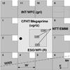 |
Fig. 1 Pointings of the INT, CFHT and ESO imaging data sets together with the filters used, and the three EMMI spectroscopic fields. The position of MACS J2243, the supercluster centre, is indicated by the black dot. It was unknown by the time the quasi-simultaneous CFHT and INT observations were performed. The layout of the 4 CCDs in the WFC/INT detector array is indicated for the upper right pointing. The area above the dash-dotted line is covered by SDSS-DR7. |
2. Observations and data reduction
All images were processed with THELI2 (Erben et al. 2005). The instrumental signature was removed through overscan correction, debiasing, flat-fielding and, if necessary, defringing. After fixing astrometry and photometry, the sky was subtracted and the data combined into mosaics. Particularities in the data reduction are explained below. The various pointings on sky are shown in Fig. 1, and their characteristics are summarised in Table 2.
2.1. 2.2 m MPG-ESO/WFI imaging
The initial shear-selection discovery of SCL2243 was done with archival R-band data taken 2000-08-28/29 in clear and good seeing conditions with the Wide Field Imager (WFI) at the 2.2 m MPG-ESO telescope in La Silla, Chile. The objective of the programme (165.S-0187) was a TNO search; no TNO was found in that field (Hainaut, priv. comm.). The data were identified by us in the ESO archive using the Querator3 tool. It was developed in the course of our ASTROVIRTEL proposal, allowing for a more specific data mining of the ESO archive returning fields suitable for weak lensing purposes (in this case identifying data sets with sub-arcsec seeing conditions and a certain minimum total integration time in R-band). More details can be found in Schirmer et al. (2007) and Micol et al. (2004). WFI has a field of view of 34′ × 34′with a pixel scale of 0.′′238.
An absolute photometric calibration was not done as it was not necessary for our initial single-band weak lensing survey. We simply adopted the standard instrumental ZP for R-band, yielding a 5σ depth of Rlim ~ 24.7 mag.
2.2. CFHT/Megaprime imaging and photometric redshifts
With the moderate depth of the single-band WFI data and only a crude magnitude cut for the selection of lensed background galaxies, our weak lensing analysis of clusters at z ~ 0.45 was limited. To cover a larger area and to refine the weak lensing measurements, we obtained CFHT/Megaprime ugriz images in excellent and photometric seeing conditions through Opticon proposal 2008BO01, with a pixel scale of 0.′′186. The pointing for CFHT was chosen to fully cover the WFI field (see Fig. 1). We did not centre it on the WFI pointing to keep bright stars outside the field of view.
Images were pre-reduced using ELIXIR (Magnier & Cuillandre 2004) at CFHT, including corrections for scattered light on the order of 0.1 mag. The remaining processing was done with THELI following Erben et al. (2009). Astrometry and relative photometry was performed using Scamp (Bertin 2006), processing all filters at the same time and thus guaranteeing a common distortion correction and pixel grid for all coadded images. For the absolute flux calibration we adopted the standard ELIXIR zeropoints as data were taken in photometric conditions. Zeropoints were refined during the photometric redshift calibration (see Sect. 2.2.2).
Characteristics of the MPG-ESO/WFI, CFHT/Megaprime and INT/WFC data.
2.2.1. Asteroid masking: an outlier rejection filter for SWarp
SCL2243 is projected near the ecliptic, resulting in a large number of asteroid tracks in the images. This is problematic as the fainter ones with low proper motion can be mistaken for highly elongated (i.e. significantly sheared) background galaxies. For the single-band MPG-ESO/WFI data asteroids were removed manually from the object catalogue obtained from the coadded image. Manual cleaning became unfeasible for our multi-colour CFHT and INT observations with 16 times larger sky coverage. Instead of working on the catalogue level, we developed an advanced outlier rejection filter which operates on the individual resampled images before image combination. In this way a coadded image free from asteroid tracks is created, providing a much cleaner basis to work with. As this tool is a recent implementation in THELI and not described in Erben et al. (2005), we provide more details in the following.
The working principle of the filter is as follows. THELI uses SWarp (Bertin et al. 2002) to resample images to a common grid on sky and to perform the final image coaddition. During the resampling process all astrometric corrections and projections are applied, meaning that a particular pixel in one exposure covers a well-defined area on sky. Precisely the same area is covered by the other (resampled) pixels in subsequent exposures. The standard procedure in SWarp is to calculate a weighted mean from the resampled pixels to estimate the flux in the coadded image,  (1)Here Ii is the flux of the resampled pixel in the ith exposure, fi a flux correction factor (containing exposure times and relative photometric zeropoints), and wi an individual weight calculated from the normalised flat, sky noise and fi (see Sect. 7 in Erben et al. 2005, for details). Whereas all the information is at hand, SWarp (as of version 2.19) has no internal outlier rejection implemented. However, we can work around this by identifying bad pixels externally and setting them to zero in the weight maps before Swarp performs the weighted image combination. In this manner we do not interfere with the internal processing of Swarp, automatically preserve photometry and do not introduce biases.
To identify the bad pixels, we reconstruct the pixel stacks from the resampled images. Ignoring the highest and lowest pixel values in the stack, we calculate the standard deviation and, in a first pass, apply a classic κ − σ-clipping to identify bad pixels and asteroids. To mask fainter asteroids we have to use comparatively low values of κ ~ 3 − 4. This results in zealous masking of healthy pixels in the presence of non-Gaussian (Poissonian) noise and small stack sizes. However, since the PSF is well sampled and since the images were resampled by a broad Lanczos3 kernel, an asteroid causing a bad pixel will also spoil the neighbouring pixels. Therefore, in a second pass, THELI only masks a bad pixel if at least n of the 8 surrounding pixels were initially also recognised as bad (n is a user-supplied parameter and we find that n = 4 − 6 works well). With this clustering analysis we identify and mask asteroids only while preserving the noise properties of the rest of the image. Optionally, pixels adjacent to a cluster of bad pixels can also be masked, which helps removing the haloes of very bright asteroids. See Fig. 2 for an example.
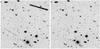 |
Fig. 2 Left: coadded CFHT r-band image without asteroid filtering. Right: using the rejection algorithm described in Sect. 2.2.1. |
2.2.2. Photometric redshifts
Photometric redshifts were obtained as outlined in Hildebrandt et al. (2009), with some modifications as outlined in the following. Prior to the photo-z determination, the PSF in all filters was homogenised and also brought to a Gaussian shape. This method will be described in a forthcoming paper (Kuijken et al., in prep.). Our experience with CFHTLS (Erben et al. 2009) and deeper spectra showed that this improves in particular the photo-z estimates of faint and high redshift galaxies. The CFHT data used for the present paper are very similar to those of CFHTLS, hence it is plausible to assume that they profited from the PSF homogenisation in a similar way, even though we cannot verify it due to the lack of deep spectroscopic coverage.
Using 89 SDSS (Adelman-McCarthy et al. 2008) and 101 NTT/EMMI spectra, we re-calibrated the photometric zeropoints of the CFHT/Megaprime images. Only sources with photometric errors smaller than 0.1 mag in all bands were used for this purpose. In detail, we fix the redshifts of the corresponding galaxies to their spectroscopically determined values. The average magnitude differences between the best-fit templates and the observed photometry are zero within errors, with exception of g-band (0.047 mag, demonstrating the excellent photometric calibration using ELIXIR). The photo-z uncertainty is σΔz ~ 0.04 (1 + z)-1, identical to the one for our reduction of the CFHTLS fields (Erben et al. 2009).
2.3. INT/WFC imaging
To probe the outer regions of SCL2243 we observed 12 adjacent pointings in gri filters using the wide field camera (WFC) at the 2.5 m Isaac Newton Telescope (INT) in La Palma, Spain. INT/WFC has four detectors forming an asymmetric focal plane (see upper right of Fig. 1), covering 34′ × 34′ on sky with a pixel scale of 0.′′331. INT/WFC cannot be used for weak lensing due to its large pixels and image quality. The latter is degraded by dome seeing, a non-coplanar detector arrangement, and sometimes by tracking instabilities. Sub-arcsecond image seeing is infrequently achieved with INT/WFC. However, it is a good photometric instrument with high throughput and thus well suited for our survey of SCL2243.
Data were taken mostly in photometric conditions in 2008-10-24 to 2008-10-27, 2008-11-16 and in 2009-10-14 to 2009-10-16 through CAT-ID 2008B/C11 and 2009B/C01. Images are shallower than the CFHT data (see Table 2) due to shorter exposure times and worse seeing conditions. Pointings 1 and 2 in gi filters were affected by 3′′ seeing, pointing 3 by 2′′. This resulted in a degradation of image depth by 0.8 and 1.0 mag for g and i, respectively, as compared to the values listed in Table 2. The data are still deep enough to probe the red sequence at z = 0.45. However, the very large seeing differences between filters gri made accurate colour measurements for pointings 1 and 2 difficult despite our attempt to homogenise the PSF, resulting in reduced number densities for these pointings.
The astrometric and relative photometric calibration was performed similar to the CFHT images, calibrating all images simultaneously. Since the illumination correction for WFC/INT is unknown, we determined the ZPs for each of the four detectors independently through direct comparison with SDSS. Variations between chips are ≤ 0.02 mag. Only the southernmost 10′ − 20′ of pointings 3 − 6 are not covered by SDSS (Fig. 1). Detectors in these areas were calibrated using average correction terms determined from the other pointings with full SDSS overlap. In this way homogeneous photometry is achieved across all 12 pointings. For better comparison with the CFHT data we determined average corrections from the overlap areas, ![Mathematical equation: \begin{eqnarray} &&\langle g_{\rm CFHT} - g_{\rm INT}\rangle = -0.09\;{\rm mag} \\[2.7mm] &&\langle r_{\rm CFHT} - r_{\rm INT}\rangle = +0.07\;{\rm mag} \\[2.7mm] &&\langle i_{\rm CFHT} - i_{\rm INT}\rangle = +0.14\;{\rm mag} \arraycolsep1.75pt \end{eqnarray}](/articles/aa/full_html/2011/08/aa16348-10/aa16348-10-eq107.png) and applied these to the INT zeropoints.
and applied these to the INT zeropoints.
As can be seen from Fig. 1, the sky coverage with WFC/INT is not complete due to the asymmetric detector layout. We checked the corresponding areas in SDSS to ensure that we did not miss any potential further member clusters.
2.4. Catalogues
2.4.1. Photometric catalogues and masking
The photometric catalogues were created as follows. After PSF homogenisation we used SExtractor (Bertin & Arnouts 1996) in double image mode, using the i-band image for the detection channel and the individual filter stacks for photometry (for the INT data a noise-normalised stack of the gri images served as the detection channel). In this way the object flux in each filter was integrated over identical apertures. We kept objects with at least 5 connected pixels with S/N ≥ 1.5 each. Objects near brighter stars were removed using the automask tool (Dietrich et al. 2007; Erben et al. 2009).
2.4.2. Shear catalogue
The shear catalogue is based on a noise-normalised combination of the CFHT r- and i-band images for extra depth. SExtractor detections with a minimum number of 5 connected pixels with S/N ≥ 2.0 form the primary catalogue. The latter was fed into our implementation (Erben et al. 2001) of the KSB method (Kaiser et al. 1995; Luppino & Kaiser 1997; Hoekstra et al. 1998) for shape measurement. A description of the PSF correction can be found in Bartelmann & Schneider (2001).
Objects with a low KSB detection significance (νmax < 10) or a PSF corrected modulus of the ellipticity larger than 1.5 are removed from the catalogue (the ellipticity can become larger than 1 due to the PSF correction). We also reject galaxies for which the correction factor (Tr Pg)-1 > 5 (Erben et al. 2001). More details about this can be found in Schirmer et al. (2007).
To remove unlensed foreground objects we kept galaxies with zphot > 0.5 only. The number density of lensed galaxies after filtering is n = 19.5 arcmin-2, and the width of the ellipticity distribution σ|ε| = 0.37. Both n and σ|ε| determine the S/N of the weak lensing analysis. The unweighted mean (median) photometric redshift of the shear catalog is ⟨ z ⟩ = 1.15 (1.00).
2.5. NTT/EMMI spectroscopy
Multi-object spectroscopy for the three most promising shear-selected clusters in the MPG-ESO/WFI data was taken with NTT/EMMI (ESO/La Silla) in 2007-08-21/22 in sub-arcsecond seeing conditions. We covered the 3800 − 9500 Å wavelength range with a spectral resolution of 3.′′6 Å pixel-1. About 40 slitlets, 1.′′3 wide, were placed in each of the three slit masks. Exposure times were 6 × 1800 s for the northern-most field, and 4 × 1800 s for the other two pointings.
The data were reduced using a custom pipeline which will be described in a forthcoming paper. In short, the data were overscan corrected, debiased and flat-fielded. We corrected for spatial distortions of the spectral footprints and small rotations of the slitlets, and subtracted a background model. Wavelength calibration was done based on combined helium/argon arc lamps. The pre-processed spectra were combined using a weighted average, and 1D-spectra were extracted. Flux-calibration and correction for telluric absorption were not performed. The redshift determination was done using [OII] 3728, Hβ 4862, [OIII] 5007 and Hα 6564 emission lines, as well as CaII 3934/3969, G-band (4305 Å), Mg 5177 and E-band (5269 Å) absorption features.
3. Measuring mass and light in SCL2243
3.1. Selection and distribution of early-type galaxies
Early-type galaxies form preferentially in high-density cluster environments through interaction with neighbours and the stripping of intra-galactic gas (see e.g. Quilis et al. 2000; Parry et al. 2009; Scannapieco et al. 2009). However, observations show that star formation is already enhanced in much less dense environments at clustercentric distances of several virial radii, consuming the gas available for further star formation. The latter is then subdued quickly with increasing proximity to denser clusters and filaments. Therefore we expect to find an increasing fraction of passive redder galaxies with colours similar to those of early-type galaxies in regions with enhanced mass density (see Gerken et al. 2004; Porter & Raychaudhury 2007; Tanaka et al. 2007; Porter et al. 2008; Verdugo et al. 2008, for further details and observational evidence). Consequently, by selecting galaxies with early-type colours we should be able to not only identify the main clusters in SCL2243, but also to map the connecting skeleton over large distances. This turned out to work well as we show in the following. In a second step, we create a 2-dimensional map of the luminosity density (Sect. 3.3) based on the distribution and fluxes of the sample of early-type galaxies, and use it as a guide for our weak lensing mass integration along the filaments (see Sect. 3.6 for details).
Our sample of elliptical galaxies is extracted from a g − r vs. r − i colour–colour diagram. We overplot member galaxies of MACS J2243 (Fig. 3, red dots) and in this way determine the selection criteria for early-type galaxies as ![Mathematical equation: \begin{eqnarray} \label{selcrit0} &&0.40 \leq z_{\rm{phot}} \leq 0.52 \\[2.7mm] \label{selcrit1} &&1.40 \leq g-r \leq 1.80 \\[2.7mm] \label{selcrit2} &&0.62 \leq r-i \leq 0.78 \\[2.7mm] \label{selcrit3} &&2.0\,(r-i) \leq g-r \leq 2.0\,(r-i) + 0.4\,. \arraycolsep1.75pt \end{eqnarray}](/articles/aa/full_html/2011/08/aa16348-10/aa16348-10-eq129.png) Equation (5) covers the 1σ uncertainty around the mean photometric cluster redshift of 0.46 (slightly higher than the spectroscopic value of 0.45). The remaining criteria are visualised in Fig. 3. In addition, we adopted a lower limit of i ≤ 22 mag (Mi ≤ − 19.3 at z = 0.45) to reject high-z interlopers. Note that these criteria are partially redundant as Eqs. (6) to (8) already perform a good selection in redshift, sufficient to select mainly early-type galaxies in the desired redshift range for the 12 INT/WFC pointings. The latter were observed in gri filters only and thus have no photometric redshifts. 2507 early-type galaxies with i ≤ 22 and suitable photometric redshifts (respectively colours) remain in the full field, 857 of which lie inside the CFHT field. For comparison, inside the CFHT area 1664 late-type galaxies with 0.40 ≤ zphot ≤ 0.52 and i ≤ 22 are found.
Equation (5) covers the 1σ uncertainty around the mean photometric cluster redshift of 0.46 (slightly higher than the spectroscopic value of 0.45). The remaining criteria are visualised in Fig. 3. In addition, we adopted a lower limit of i ≤ 22 mag (Mi ≤ − 19.3 at z = 0.45) to reject high-z interlopers. Note that these criteria are partially redundant as Eqs. (6) to (8) already perform a good selection in redshift, sufficient to select mainly early-type galaxies in the desired redshift range for the 12 INT/WFC pointings. The latter were observed in gri filters only and thus have no photometric redshifts. 2507 early-type galaxies with i ≤ 22 and suitable photometric redshifts (respectively colours) remain in the full field, 857 of which lie inside the CFHT field. For comparison, inside the CFHT area 1664 late-type galaxies with 0.40 ≤ zphot ≤ 0.52 and i ≤ 22 are found.
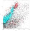 |
Fig. 3 g − r vs. r − i colour–colour diagram. Red dots: galaxies with distances smaller than 1.8 Mpc from of the supercluster centre. The box outlines our photometric selection criteria for early-type galaxies (Eqs. (6) to (8)) in the supercluster. Blue dots: galaxies with 0.27 ≤ zphot ≤ 0.39 from the full CFHT field. |
The spatial distribution of these galaxies is shown in Fig. 4 (small black dots). Large red dots indicate galaxies for which we have matching SDSS spectra (full field) and EMMI spectra (peaks G, H, I, and J). The central cluster (MACS J2243, labelled A) forms a highly significant overdensity. Within the CFHT field we select 10 clusters or overdensities, based on a minimum peak luminosity density of 1010.1 L⊙ Mpc-2. For WFC/INT we present the four most promising clusters only, as part of the area is contaminated with foreground structures at z = 0.36−0.39. We cannot unambiguously separate these from smaller overdensities at z ~ 0.45. Our cluster detections are listed in Table 3. Half of these do not form typical clusters but loose associtations of galaxies (see also the images in the appendix).
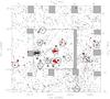 |
Fig. 4 Distribution of early-type galaxies with z ~ 0.45. Sky coverage is incomplete, as is indicated by the shaded areas (rectangular: gaps due to telescope pointing, circular: bright stars). The dashed line indicates the CFHT field of view. The reduced number density of objects left of the CFHT field is caused by strongly varying seeing conditions which made precise colour measurements very difficult (see Sect. 2.3 for details). Empty circles mark member clusters of overdensities, their size qualitatively indicating richness. |
3.2. Luminosity-based r200 and M200 of MACS J2243
K-corrections and rest-frame luminosities in i-band were calculated using kcorrect v4.2 (Blanton & Roweis 2007). As we have projected the filter transmission curves to the main cluster redshift of z = 0.45, we denote them as e.g. 0.45i. Since kcorrect evaluates luminosities for h100 = 1.0, we corrected the absolute magnitudes by 5log 10(h100 = 0.7) ~ −0.77 mag.
Hansen et al. (2005) and Johnston et al. (2007) have shown that r200 and M200 can be estimated from the number Ngal of galaxies within a radius of  Mpc of the brightest cluster galaxy (BCG). Only galaxies in the red sequence and with i-band luminosities L > 0.4 L∗ are considered. The refined version from the relation of Hansen et al. (2005) reads
 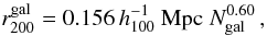 (9)being the radius within which the luminosity is 200 times the mean luminosity of the Universe. It must not be mistaken for r200 which refers to matter overdensity. Based on weak lensing measurements and the number N200 of galaxies within
  , Johnston et al. (2007) and Hansen et al. (2009) obtain
 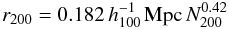 (10)
(10) (11)
(11)
List of possible member clusters and sub-structures.
Fitting a Schechter-type luminosity function (Schechter 1976) to the early-type galaxies in MACS J2243, we determine  mag (see Fig. 5) and
  . Using Eqs. (10) and (11) we find for the central cluster MACS J2243
  (12)
(12) (13)
(13) (14)
(14)
3.3. The luminosity map of the central square degree
For our analysis of the light distribution in SCL2243 we smooth the luminosity field of the early-type galaxies with a FWHM = 4′ wide Gaussian kernel, corresponding to a physical scale of  Mpc at z = 0.45. The kernel is truncated at a radius of 2σ and has a constant value subtracted such that it becomes equal to zero at r = 2σ (and it is normalised). In this way we suppress the effects of the broad wings. This kernel is significantly smaller than the smoothing radius of
  Mpc chosen by Einasto et al. (2007b) in their search for superclusters (using an Epanechnikov kernel which has steeper edges than our Gaussian filter). The purpose of their work was to identify superclusters in a large volume, whereas we are interested in the internal structure of SCL2243.
We show the luminosity density of the CFHT field in Fig. 6, overlaid as green contours over the distribution of early-type galaxies (black dots). Contour levels increase in logarithmic steps of 0.3. Red dots are spectroscopically confirmed member galaxies, three from SDSS in the main cluster, and all but two of the rest from NTT/EMMI. Dots with cyan colours belong to a foreground cluster at z = 0.326. Blue contours represent the weak lensing mass reconstruction (see Sect. 3.5).
SCL2243-J (see Table 3) is masked from all subsequent analyses at it is projected behind a foreground cluster at z = 0.326. We recognise three filaments connected to MACS J2243, which we call AC, AH and AFDGI according to the labelling we chose for the sub-structures identified (Fig. 4). These structures extend over (5 − 15) h-1 Mpc. We predict at least one more filament South-East of MACS J2243, connecting to SCL2243-B (Fig. 4). The characteristic width of all filaments is about  Mpc, with local enhancements up to ~ 3.0 Mpc where concentrations of galaxies or small member clusters are found.
We measure a total luminosity of early-type galaxies in the CFHT field of  . Within r200 the luminosity of MACS J2243 is (3.60 ± 0.11) × 1012L⊙, whereas filaments AC, AH and AFDGI contribute (5.19 ± 0.31) × 1012 L⊙.
3.4. Colour variations within the supercluster structure
Figure 7 displays the unweighted ⟨ g − i ⟩ colours of all galaxies with 0.40 ≤ zphot ≤ 0.52 and i < 22 mag. For visual reference we overlaid the luminosity contours of the early-type galaxies tracing the supercluster structure. MACS J2243 is the most massive object and thus also the one with the reddest colour (g − i = 2.27 mag) at its centre. At a clustercentric distance of 0.25 × r200, g − i starts decreasing, reaching 1.90 ± 0.05 mag at the virial radius.
This is not much redder than filaments AC and AFDGI with ⟨ g − i ⟩ = 1.80 (0.05 mag scattering). These filaments become redder by about 0.05 mag in areas of greater density (objects C, D, F, G, and I), but are otherwise remarkably constant out to distances as large as 6 × r200 (even 8 × r200 or 18 Mpc if SCL2243-K is spectroscopically confirmed). Also, the colour of different filaments is the same with one exception: the middle of filament AH is noticably bluer, ⟨ g − i ⟩ = 1.71 ± 0.02 mag.
Filaments AH and AF merge before connecting to the western-most side of cluster A. This area is significantly redder by 0.08 mag forming a cluster infall region. Objects E, H and J appear further evolved than the rest of the field with g − i = 2.0 mag (E, H) and 1.9 mag (J), respectively.
3.5. The mass map of the central square degree
Weak gravitational lensing has been used with great success when mapping the matter distribution and density profiles of clusters of galaxies (see Dahle 2007, for a listing). In this paper we use the model-free finite-field method from Seitz & Schneider (2001) to reconstruct the dimensionless surface mass density, κ. This method uses the field border as a boundary condition and is easily implemented for rectangular data fields4.
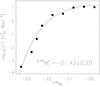 |
Fig. 5 Rest-frame 0.45i-band luminosity function for the early-type galaxies within r200 = 2.06 Mpc of the supercluster centre. The solid line shows the best-fit Schechter model. |
Mass reconstruction algorithms must operate on smoothed shear fields as otherwise noise contributions become infinite (Kaiser & Squires 1993). We chose the same truncated Gaussian filter as for the luminosity field (Sect. 3.3), with an identical width of 4.′0 and a constant value subtracted such that the filter becomes zero at the maximum radius of 2σ. This zero-setting of the filter is a requirement for the Seitz & Schneider (2001) algorithm as it ensures that the derivatives of the smoothed shear field are well-behaved.
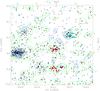 |
Fig. 6 Early-type galaxies with 0.40 ≤ zphot ≤ 0.52 (black dots). Overlaid are galaxies with EMMI and SDSS spectra within 0.43 < zspec < 0.46 (red dots). Blue dots with black circles have 0.32 < zspec < 0.33. The cluster at RA = 340.2 Dec = −9.35 is a foreground object (z = 0.326) superimposed over a sub-structure at z = 0.456. The solid blue contours represent the S/N of the mass reconstruction, starting at 2σ and increasing in steps of 1.0σ; dashed contours represent negative values (2σ and 3σ). Green contours trace the smoothed luminosity density I (in Li, ⊙ Mpc-2) of the early-type member galaxies in logarithmic units, starting with Log10(I) = 9.6 and increasing in steps of 0.3. The smoothing length for the surface mass density and luminosity density was 4.′0. The upper and right axes give the physical scale at the main cluster redshift of z = 0.447. Compare to Fig. B.1 in the appendix for late-type galaxies in the same redshift range. |
The reconstruction algorithm only works for under-critical regions with κ < 1, i.e. strong lensing areas are not reconstructed reliably. This is of no concern for our work as the smoothing scale is significantly larger than the strong lensing regions in the core of MACS J2243.
The convergence κ is determined up to an additive constant, the so-called “mass-sheet degeneracy”, which is broken by assuming that κ vanishes on average along the border of the field. We excluded part of the edge close to MACS J2243 to avoid biasing by increased values of κ in this area. The uncertainty in the determination of the mass sheet degeneracy can be estimated from the variations along the edge in randomisations (see below) and the number of independent apertures that can be placed along the border. The uncertainty of the mass sheet degeneracy correction term is σκ = 0.0023.
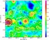 |
Fig. 7 The g − i colours of all galaxies (early- and late-type) with 0.40 ≤ zphot ≤ 0.52. For visual reference we overlaid the luminosity contours of the early-type galaxies tracing the structure of the supercluster, and the mass reconstruction (thin solid black lines, this time starting at 1σ). The black dashed contours represent negative mass reconstruction levels (2σ and 3σ). The thick black circle marks r200, its width indicates the 1σ uncertainty. |
The noise level of the mass reconstruction mainly depends on two quantities: the width of the distribution of intrinsic ellipticities (σ|ε| = 0.37) and the local number density of background galaxies. The latter would in principle be fairly constant if it was not significantly altered by the masks we put on top of brighter stars. To obtain the noise map, we created 1000 realisations of randomised galaxy orientations keeping their positions fixed and reconstructed the κ-field for each of them. The two-dimensional rms of these κ-maps then yields the desired noise map. Since lensing increases the ellipticities of galaxies, we removed the radially averaged tangential shear profile of MACS J2243 prior to the randomisations. Otherwise the noise at the cluster position would be overestimated. This correction is only significant for the supercluster core (improving its S/N by about 10%), and negligible for all other mass concentrations as their noise is dominated by intrinsic ellipticities. The resulting mass map is overplotted (blue respectively black contours) over the luminosity and colour maps shown in Figs. 6 and 7.
We detect MACS J2243 at the 10σ level and estimate  (15)
(15) (16)This is in very good agreement with our earlier luminosity-based analysis in Sect. 3.2, yielding
  and
and  , respectively.
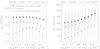 |
Fig. 8 Filaments have not yet been detected directly with weak lensing. However, we can attempt to integrate the weak lensing reconstructed surface mass density κ within different isophotes, yielding a statistically significant measurement due to the increased area. Left: the total mass in the filaments obtained by integrating κ, with and without condensations in the filaments (crosses and diamonds, respectively). For comparison we show the total, including the supercluster centre (black dots). More details in the text. Error bars were calculated from the 1000 randomised data fields. Right: same as the left panel, but for the M/L ratio. |
3.6. Weak lensing and filaments
Weak gravitational lensing has so far been hitting a limit when it comes to the direct detection of filaments, as their density is significantly lower and their extent much larger than those of galaxy clusters. Gray et al. (2002) reported a ground-based weak lensing detection of a small filament in A901/902, which could not be confirmed by HST/ACS observations (Heymans et al. 2008). Likewise, Kaiser et al. (1998) found a filament in MS0302, but argued it could be due to projection effects from structures elsewhere along the line of sight. This feature was not seen by Gavazzi et al. (2004). Similarly, Dietrich et al. (2005) reported a weakly significant lensing detection of a filament connecting the close double clusters A222/223. They have argued, however, that it is difficult to disentangle the shear signals of the close pair of clusters from that of the filament.
Note that all these filaments are very small with lengths on the order of  Mpc, connecting very close clusters, whereas the filaments we study in SCL2243 are approximately one order of magnitude larger, representing the actual cosmic web.
Mead et al. (2010) have discuss the subject of (cosmic web) filament weak lensing based on simulations. They have investigated three possible measurement methods, one of them being the direct approach of model-free mass reconstruction using the same technique as we do in this paper. They have found that filaments are in general difficult to detect given their low surface mass density (κ ~ 0.01). With number densities of 30 galaxies arcmin-2 typical for very deep ground-based imaging, even the most massive filaments were only weakly detected. Space-based observations yield about three times higher number densities, which improve detection statistics.
3.6.1. Weighing supercluster filaments with weak lensing
The direct detection of filaments in a supercluster with weak lensing is a difficult task and has so far not been achieved. This also holds for our data set, as we only detect the most massive concentrations in the filaments with S/N ~ 3 − 4 in the mass reconstruction.
However, absence of detection does not mean absence of signal. As we have summarised at the beginning of Sect. 3.1, early-type galaxies serve as a good tracer for the underlying distribution of gravitating matter. Therefore one would expect a trend towards positive values of κ wherever early-type galaxies dominate the field. Indeed we see a correlation of κ with the galaxy distribution at the S/N ~ 1 − 2 contour level, in particular along the filament DFGIK, and in general where the galaxy population has colours larger than about 1.7 (Fig. 7).
At a given point on sky this is of course insignificant. But by integrating κ over areas where the smoothed luminosity or colour exceeds a certain value, we can arrive at a statistically significant measurement. This is equivalent to the statistical stacking of weak lensing signals, in order to make a measurement that would otherwise be unfeasible, or to obtain high-S/N statistics (e.g. Hoekstra et al. 2001; Parker et al. 2005; Sheldon et al. 2004, 2009). The results of this measurement are shown in Fig. 8, where we integrated κ over areas with different isophotes. Our analysis is restricted to the region covered by the supercluster centre and filaments AC, AH, and AFDGI. We have repeated it three times, integrating over
-
the entire supercluster;
-
the filaments only;
-
the filaments only, excluding mass concentrations with S/N(κ) > = 2.
To better understand the plots in Fig. 8 one must note that for very low isophotal boundaries one integrates over a larger area. This increases the noise and also includes underdense regions with negative κ. This is felt mostly by the naked filaments (i.e. without contribution from embedded clusters or overdensities), thus the integrated mass for the lower curve (left panel, diamonds) decreases. Isophotes brighter than ~ 109.8 − 9.9 L⊙ Mpc-2 cover increasingly smaller areas and thus smoothing effects become important, distributing mass and light to areas outside those contours. Of course the smaller integration area also leads to decreased mass estimates. In addition, due to characteristic positional uncertainties of 1′ − 2′ in the mass reconstruction (due to noise, see e.g. Schirmer et al. 2007), the surface mass density field starts to decouple from the luminosity field. As a consequence of the latter three effects, mass estimates decrease significantly if the integration contour is too tight (higher than about ~ 109.8 − 9.9 L⊙ Mpc-2 for our data). The same effects hold for the M/L ratio (right panel of Fig. 8). For the discussion below (Sect. 4.2.4) we constrain our analysis of the filaments’ mass and M/L ratio to two different isophotal levels, I1 = I200 and I2 = 0.5 × I200, where I200 is the average luminosity density at the virial radius of the supercluster core.
4. Discussion and results
4.1. Supercluster constituents and extent
Using early-type galaxies we have mapped SCL2243 over four square degrees. Its extent in East-West is  Mpc, whereas it appears more compact North-South (
 Mpc). If future spectroscopic observations confirm further objects from Table 3, the latter figure could increase to ~
  Mpc. The redshift range of 0.435 − 0.456 suggests an extension of about 50 Mpc along the line of sight. This makes SCL2243 the largest supercluster known at intermediate redshifts (Table 1). Only J1000+0231 at z ~ 0.7 in the COSMOS field has an extent of 400 Mpc along the line sight (Guzzo et al. 2007), but one may argue that this is due to a projection of three unconnected smaller structures.
The supercluster centre is formed by a massive galaxy cluster, SCL2243-A (MACS J2243 Ebeling et al. 2010), with  Mpc, N200 = 150 ± 30 and M200 = (1.54 ± 0.29) × 1015 M⊙. It shows significant sub-structuring, several strongly lensed galaxies and is not in dynamic equilibrium (see Fig. C.1 for an image). More details about this spectacular cluster will be published elsewhere (M. Bradač, priv. comm.).
The outer parts of SCL2243 are characterised by five individual clusters, SCL2243-B, H, M, N and L (Fig. 4). The latter two still need spectroscopic confirmation. The remaining objects listed in Table 3 have very low concentration and do not exhibit an obvious centre or a characteristic brightest cluster galaxy. SCL2243-D, F, G, I (and K) form a 15 − 20 Mpc long filament rich in early-type galaxies, but therein they hardly represent more than just density variations. This pearl necklace appearance is typical for inter-cluster filaments and commonly seen in simulations (Aragón-Calvo et al. 2010).
Properties of the various supercluster components, integrated within two different isophotal contours Iiso: 1.0 and 0.5 times the average luminosity  at the supercluster virial radius. The latter covers a ~2.6 times larger area than the former.
SCL2243-C (Fig. C.3) has ~30 early-type galaxies, but lacks a clear cluster centre. Yet it forms the second highest weak lensing peak after MACS J2243. Actually, SCL2243-J has a stronger lensing signal, but this is due to a foreground cluster at z = 0.326. SCL2243-C could be a filament oriented along the line of sight. If it stretches over 10 − 20 Mpc or more, then cosmic expansion should lead to a characteristic broadening of the redshift distribution distinguishing it from a virialised cluster.
The only typical galaxy cluster in addition to MACS J2243 inside the CFHT field is SCL2243-H. It is about 0.2 mag redder than the filaments (and 0.2 mag bluer than MACS J2243) and has two bright and merging ellipticals at its core (Fig. C.5). We spectroscopically confirmed 15 galaxies in this cluster.
4.2. Mass, light and colour of the cosmic web
SCL2243 is an ideal laboratory to study the cosmic web. At a redshift of 0.45 and with an extent of two degrees it can easily be probed by current wide field imagers 7 − 8 mag beyond the brightest cluster galaxies. The intermediate cluster redshift makes it a good target for weak lensing analyses.
4.2.1. The supercluster centre: a normal but massive cluster
For MACS J2243 we find excellent agreement for r200 and M200 between weak lensing and cluster scaling relations (Johnston et al. 2007; Hansen et al. 2009). Its location at the centre of a supercluster does not appear to alter its properties as compared to other clusters in the MaxBCG sample. Its M/L ~ 428 ± 82 is in perfect agreement with those measured by Sheldon et al. (2009) for the MaxBCG cluster sample (see their Fig. 9), with more massive clusters having higher M/L ratios. This is expected as very massive clusters arise preferentially at the intersection of two or more cosmic filaments (Colberg et al. 2005; Aragón-Calvo et al. 2010), forming supercluster systems like SCL2243.
4.2.2. Width and length of the filaments in SCL2243
The global appearance of SCL2243, having a supermassive cluster at the centre as well as several normal-sized clusters and filaments with distinct density variations, is very characteristic (Aragón-Calvo et al. 2010). The typical width of the three filaments is  Mpc with local variations up to 3 Mpc. Choi et al. (2010) observed similar values for a sample of high and low redshift filaments (z ~ 0.8 and z ~ 0.1, respectively) taken from the DEEP2 (Davis et al. 2003) and SDSS surveys. Their width distribution peaks around
  Mpc and shows only little evolution with redshift (filaments tend to become more compact with time, in agreement with ΛCDM). Aragón-Calvo et al. (2010) confirm this picture in simulations, yielding a mean width of
  Mpc. González & Padilla (2010) predict a characteristic scale radius of
  Mpc for filaments less than 30 Mpc long, increasing to 3 Mpc for longer filaments.
With lengths of Mpc the filaments in SCL2243 are well matched by those of Choi et al. (2010, see their Fig. 4 for a distribution of filament lengths). If further observations reveal that filament DFGIK connects to SCL2243-M, then it would extend over ~25 Mpc. Only 2 − 3% of the filaments found by Choi et al. (2010) stretch over even longer distances.
4.2.3. The colours of SCL2243
The evolution of galaxies is a strong function of local density. Star formation is already enhanced in filaments, triggered by the increased number of interactions with neighbouring galaxies. The consumption of gas and ram-pressure stripping quickly turn blue galaxies into passive systems with colours similar to those of red sequence galaxies (see Quilis et al. 2000; Gerken et al. 2004; Porter & Raychaudhury 2007; Tanaka et al. 2007; Porter et al. 2008; Verdugo et al. 2008, and references therein), whereas morphological changes happen on significantly longer time scales (Parry et al. 2009; Scannapieco et al. 2009).
For this reason one expects the density variation in a supercluster to be mirrored in galaxy colours, an effect we see clearly for SCL2243 (Fig. 7). The core of MACS J2243 is entirely dominated by ellipticals with ⟨ g − i ⟩ ~ 2.27. At about 0.25 × r200 or ~ 500 kpc galaxies start to become bluer, a quasi-linear trend leading to ⟨ g − i ⟩ ~ 1.90 ± 0.05 at the virial radius (2.1 Mpc). The filaments have on average a colour of 1.8 mag, with a slight reddening towards their core by 0.05 mag. To some extent this central reddening is a consequence of smoothing the data field with a 4.′0 wide kernel (about half the filament width), blending bluer field galaxies into the filaments. Thus we do not consider colour variations transverse to the filaments’ main axis further. At the location where filaments AH and AF merge and connect to the supercluster centre, we observe increased reddening (g − i ~ 1.9 mag) already 1.5 Mpc outside the virial radius.
Outside this cluster infall region the filament colours stay remarkably constant even over projected clustercentric distances as large as 15 Mpc (filament DFGI). We do observe, however, an increase in g − i by about 0.05 mag where the filaments become thicker. These locations appear correlated with higher surface mass density (Fig. 7). While this is not statistically significant for most individual overdensities, the global picture is more conclusive. 13 of the weak lensing peaks with S/N > 2 are located inside or on the edge of the filaments with g − i > 1.75 mag, whereas only four are found outside in areas with bluer colour (the g − i = 1.75 mag contour roughly divides the area of the field of view in half). The most significant peak in a blue area is caused by a background cluster at z ~ 0.7 (α = 340.37;δ = −09.32; note that we use galaxies with 0.40 ≤ zphot ≤ 0.52 only to calculate colours). When turning to negative peaks, i.e. under-dense regions, results are inverted. Eleven negative mass peaks are found in blue areas and only five within filaments. Outside the evident skeleton of SCL2243 traced by early-type galaxies, the mean colour of galaxies with 0.40 ≤ zphot ≤ 0.52 is 1.60 mag with little variation (0.05 mag).
4.2.4. Mass of the filaments
A direct and statistically significant detection of an individual filament using weak lensing is very difficult and has not yet been demonstrated (see Sect. 3.6). Nevertheless, we have shown that it is possible to constrain the mass and density of the cosmic web by summing κ over areas populated by early-type galaxies. We integrated over two arbitrarily chosen isophotes, I1 = I200 ~ 109.9 L⊙ Mpc-2 and I2 = 0.5 × I200, where I200 is the mean luminosity density at the virial radius of MACS J2243. I2 and I1 are represented by the outermost and second outermost contour lines, respectively, in Figs. 6 and 7. Within I1 only isolated overdensities in the filaments are selected. I2 on the other hand encompasses a three times larger area. Our measurement is limited to filaments AC, AH, and AFDGI, and our results are shown in Table 4.
Within I1 we find a mass of (1.1 ± 0.4) × 1015 M⊙, increasing to (1.53 ± 1.01) × 1015 M⊙ for I2. Hence these filaments contain about the same mass as MACS J2243 (M200 = (1.54 ± 0.29) × 1015 M⊙). This may sound surprising, but is predicted by ΛCDM models which identify filaments as the carriers of most of the mass in the Universe, with clusters being a close second (Aragón-Calvo et al. 2010). Similar results were obtained for the Shapley supercluster, where galaxies in the filaments contribute about twice as much mass as those in clusters (Proust et al. 2006). For comparison, simplistic linear theory yields that filaments and walls contain about 10 times as much mass as clusters (Doroshkevich 1970; Aragón-Calvo et al. 2010, for an open Λ = 0 Friedmann Universe).
The mass-to-light ratio for the SCL2243 filaments (409 ± 153) within I1 is indistinguishable from MACS J2243 (480 ± 82) and becomes smaller (305 ± 201) when integrating over the larger I2 area. The increased error is caused by integrating κ over areas further away from the filament cores where the signal is diminished.
4.2.5. Density of the filaments
We find ⟨ κ ⟩ = 0.0124 ± 0.0023 for the denser filament regions within I1, decreasing to 0.0065 ± 0.0023 when integrating over I2. This is in agreement with theoretical expectations of ⟨ κ ⟩ ~ 0.01 (Mead et al. 2010). Errors are fully dominated by the uncertainty of the mass sheet degeneracy (Sect. 3.5). Making assumptions about the three-dimensional shape of the filaments and embedded condensations, we can de-project κ and estimate the physical density. However, there are some uncertainties involved.
First, our knowledge about foreground and background matter is mostly limited to three isolated NTT/EMMI pointings. SCL2243-J was excluded from our analysis as the spectra revealed that it is located behind a foreground cluster (Table A.1). The spectra for SCL2243-H show a thin foreground sheet at z ~ 0.256, but the galaxies associated with it are field spirals and do not form a spatially concentrated structure. Their lensing impact is negligible. For SCL2243-G and -I there is no evidence for other structures along the line of sight. Scanning the CFHT field for concentrations of red sequence galaxies at other redshifts did not reveal structures projected on top of SCL2243 that could cause a measurable lensing signal. We do see very high redshift clusters at z ≳ 0.8 across the field, too distant to affect our results. Other structures, such as the cluster at α = 340.37;δ = −09.32 (z ~ 0.7, Fig. 6) or concentrations of early-type galaxies at lower photometric redshifts are not projected onto cluster filaments. Hence we assume that contamination along the line of sight does not bias our mass and density estimates significantly.
The second hurdle in estimating the physical density of a filament is the determination of its volume. The density contrast is much lower than that of clusters, for which reliable size estimators are available (Sect. 3.2). Different measures exist for a filaments’ characteristic radius, based on the galaxy distribution, the typical orbit time of a galaxy in the filament, or the shape of its density profile (Colberg et al. 2005; González & Padilla 2010). To cover these uncertainties we probe the density within the I1 and I2 contours allowing for an additional ± 0.2 Mpc error. Within I1 the filaments decompose mostly into individual isolated overdensities, for which we assume spherical shapes. The average density in units of ρcrit is 121 ± 57, about half the mean density of MACS J2243 within the same isophote (I1 is the average luminosity at r200 of MACS J2243). Within I2, the assumption of a spherical shape is invalid and we adopt a cylindrical model. The redshifts of SCL2243-F and G (z = 0.437) and MACS J2243 (z = 0.447) indicate that this filament is inclined by 60 degrees with respect to the celestial plane. SCL2243-H on the other hand is at the same redshift as MACS J2243. Thus we assume some arbitrary mean inclination of 30 degrees, resulting in ρ/ρcrit = 39 ± 29. The error bars include the uncertainties of the volume and of the mass sheet degeneracy, as well as the noise of the mass reconstruction itself. These are the mean filament densities including local overdensities.
By integrating within the same isophotes, but by excluding all regions where S/N(κ) > 2, we measure the density of the stripped filaments, i.e. the parts without local overdensities. Within I1 (I2) we have ρ/ρcrit = 27 ± 46 (7 ± 25). Both results are positive but consistent with zero. In case of I1, the uncertainty of the mass sheet degeneracy prevents a detection.
For comparison, Colberg et al. (2005) found the filament density to vary between a few and 25 times the mean density of the Universe in ΛCDM simulations. With Ωm = 0.3 this is consistent with our results (scaled in terms of ρcrit).
5. Summary
5.1. Overview
In one of the fields of our weak lensing cluster survey (Schirmer et al. 2007) we made several detections. Three of them (objects #141, 144 and 147) are associated with significant overdensities of galaxies with singular SDSS redshifts of z ~ 0.45, indicating a supercluster of galaxies. This would be the first supercluster discovered using weak gravitational lensing methods only.
Our spectroscopic follow-up with NTT/EMMI confirmed the SDSS redshift of #141 (SCL2243-J, Fig. C.7) and revealed two more galaxies at the same redshift. The bulk of the other 31 galaxies in this area belong to a foreground cluster at z = 0.326. We cannot rule out that there are more galaxies at z = 0.456, as our spectroscopic coverage is shallow (i ~ 22) and only half complete at this depth. Object #144 (SCL2243-H, Fig. C.5) was confirmed with 15 galaxies at z ~ 0.447, and #147 (SCL2243-G and I, Fig. C.4) has 19 confirmed member galaxies at z = 0.436. Depth and completeness are the same as for #141.
To map the larger extent of SCL2243 and to identify its centre we observed one square degree with CFHT/Megaprime in ugriz filters. In addition, twelve pointings were taken in gri with the 2.5 m INT/WFC (La Palma, Spain) increasing the sky coverage to four square degrees. By selecting early-type galaxies at z ~ 0.45 we detected 14 potential member clusters or overdensities (Fig. 4, Table 3), eight of which have positive spectroscopic confirmation of at least the brightest galaxy. SCL2243-B, H, L, M and N are typical galaxy clusters. Further spectroscopic confirmation is required. In particular the region between clusters K, M and N has a significantly increased density of early type galaxies as compared to the remaining inter-cluster areas (Fig. 4). This should be verified by future field spectroscopy.
Using early-type galaxies we traced the supercluster skeleton of SCL2243 over clustercentric distances of Mpc (Fig. 4). We identified three large filaments and mapped the colours of the central square degree from high to low density regions. We determined the filaments’ masses by integrating the reconstructed surface density over areas with enhanced i-band luminosity, respectively red g − i colours.
SCL2243 is the third supercluster (with more than two member clusters) next to A901/902 and MS0302 that has been studied with weak lensing. Cores of other superclusters (usually supermassive clusters) at intermediate redshift have been studied with lensing before, but this is the first time that such methods have been applied to the cosmic web in superclusters.
5.2. Main results
-
We have made the first discovery of a supercluster, SCL2243,using the shear-selection method. Interestingly, the initialdetections were made on smaller clusters located inthe supercluster filamentary network, as the supercluster centrewas outside the initial field of view.
-
SCL2243 extends over
Mpc (length, width, depth) and is one of the largest superclusters studied at intermediate redshifts. We identified 14 member clusters and overdensities, as well as three filaments extending over Mpc and possibly beyond. Almost all clusters or overdensities found in the CFHT data are embedded in filaments. We expect that better data on the surrounding INT fields will confirm this picture for the remaining clusters. -
The supercluster centre, SCL2243-A, was found at the edge of the CFHT field. With M200 = (1.3 − 1.5) × 1015 M⊙ and M/L = 428 ± 82 it is fully consistent with similar clusters in the MaxBCG sample. SCL2243-A is also contained in the massive cluster survey (Ebeling et al. 2001) and referred to as MACS J2243-0935. There is very good agreement between cluster scaling relations and weak lensing based mass and size estimates (
Mpc). -
We observe a significant correlation between the surface mass density κ and the supercluster skeleton as outlined by its i-band luminosity and g − i colours. κ is statistically insignificantly enhanced above zero for most areas, yet a global trend is visible. Motivated by this, we integrated κ over the filaments and obtained for the first time good weak lensing constraints for the cosmic web. We find a total filament mass of (1.53 ± 1.01) × 1015 M⊙, similar to M200 = (1.54 ± 0.29) × 1015 M⊙ for MACS J2243. More mass is located in another filament which we predict at the South-East of MACS J2243. The high filament mass is in agreement with ΛCDM models where most of the mass of the Universe is in filaments, with galaxy clusters being second.
-
The measured weak lensing surface mass density of the filaments is κ ~ 0.003−0.012, consistent with theoretical expectations (κ ~ 0.01). Uncertainties in the determination of the mass sheet degeneracy become the limiting factor and prevent a positive detection when we aim at the naked parts of the filament, i.e. those regions without overdensities. Depending on de-projection, these surface mass densities translate to physical densities of ρ/ρcrit ~ 10−100.
-
The M/L ratio of the filaments evaluates to 409 ± 153, very similar to that of MACS J2243 (428 ± 82), integrated within the same isophotal contour.
-
The density field in SCL2243 shows large variations which are typical for superclusters, ranging from supermassive clusters down to low contrast filaments. Correspondingly, we expect galaxy colours to change depending on their location. The supercluster core has ⟨ g − i ⟩ = 2.27 mag, dropping to 1.90 mag at r200. For the filaments we observe a constant colour of 1.80 mag, independent of clustercentric distance. Only in the cluster infall region (out to 1.5 Mpc outside r200) do the filaments become noticeably redder, having the same average colour as the supercluster centre at its virial radius. Small colour variations of 0.05 mag amplitude are observed along the filaments, coinciding with local overdensities or one of the member clusters.
SCL2243 and its massive filamentary network form a textbook supercluster. Large-scale spectroscopic coverage is required to disentangle its real 3D shape and to obtain independent mass estimates. With very deep wide-field imaging using 8 m class telescopes it should be possible to make a significantly improved weak lensing study of the filamentary network in SCL2243. Our new approach of directly probing the cosmic web with weak lensing should facilitate future lensing-based mass estimates of inter-cluster filaments.
Online material
Appendix A: Redshifts
NTT/EMMI spectroscopic redshifts of SCL2243-G and I (left), SCL2243-H (middle) and SCL2243-J (right).
Appendix B: Further plots
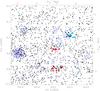 |
Fig. B.1 Same as Fig. 6, but for late-type galaxies with 0.40 ≤ zphot ≤ 0.52. Note that the filamentary supercluster structure is much less evident from these galaxies. Overlaid are galaxies with EMMI and SDSS spectra within 0.43 < zspec < 0.46 (red dots). Blue dots with black circles have 0.32 < zspec < 0.33. The cluster at RA = 340.2 Dec = −9.35 is a foreground object (z = 0.326) superimposed over a sub-structure at z = 0.456. The solid blue contours represent the S/N of the mass reconstruction, starting at 2σ and increasing in steps of 1.0σ; dashed contours represent negative values (2σ and 3σ). The smoothing length for the surface mass density was 4.′0. The upper and right axes give the physical scale at the main cluster redshift of z = 0.447. |
Appendix C: Selected cluster images
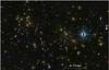 |
Fig. C.1 SCL2243-A (CFHT image). Note that this image does not cover the full extent of this cluster. The same holds for all other images below, only the central or representative parts are shown. |
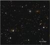 |
Fig. C.2 SCL2243-B (INT image). |
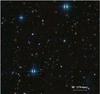 |
Fig. C.3 SCL2243-C (CFHT image). Note the sparse distribution of early-type galaxies. |
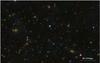 |
Fig. C.4 SCL2243-G (CFHT image). |
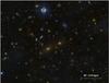 |
Fig. C.5 SCL2243-H (CFHT image). The image does not cover the full extent of this cluster. |
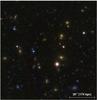 |
Fig. C.6 SCL2243-I (CFHT image). |
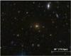 |
Fig. C.7 Part of SCL2243-J (CFHT image). The foreground cluster at z = 0.326 is outside the field of view. |
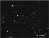 |
Fig. C.8 SCL2243-L (INT image). |
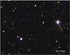 |
Fig. C.9 Part of SCL2243-M (INT image). |
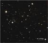 |
Fig. C.10 SCL2243-N (INT image). |
These are all objects found searching for the term supercluster in publications between 1995 and 2010, and in referenced papers.
THELI is freely available at http://www.astro.uni-bonn.de/~theli
Our implementation of this algorithm is available at http://www.astro.uni-bonn.de/~mischa/download/massrec.tar
Acknowledgments
M.S. thanks Catherine Heymans, Karianne Holhjem, Lindsay King, Emilio Pastor Mira, Peter Schneider, and the anonymous referee for discussions and suggestions which improved this paper. The authors wish to recognise and acknowledge the very significant cultural role and reverence that the summit of Mauna Kea has always had within the indigenous Hawaiian community. We are most fortunate to have the opportunity to conduct observations from this mountain. M.S. acknowledges support by the German Ministry for Science and Education (BMBF) through DESY under the project 05AV5PDA/3 and the Deutsche Forschungsgemeinschaft (DFG) in the frame of the Schwerpunktprogramm SPP 1177 “Galaxy Evolution”. H.H. is supported by the DUEL-RTN, MRTN-CT-2006-036133, the Marie Curie individual fellowship PIOF-GA-2009-252760, and a CITA National Fellowship. T.E. is supported by the German Ministry for Science and Education (BMBF) through the DESY project “GAVO III” and by the Deutsche Forschungsgemeinschaft through project ER 327/3-1 and the Transregional Collaborative Research Centre TR 33 − “The Dark Universe”.
Author contributions: M.S. obtained the CFHT, INT and NTT data, reduced the INT images and NTT spectra, and performed all scientific analyses. H.H. derived the photometric redshifts based on CFHT data. K.K. developed the PSF Gaussianisation code used in the photometry that led to the photometric redshifts. T.E. stacked the Elixir pre-processed CFHT ugriz images.
This research has made use of the VizieR catalogue access tool, CDS, Strasbourg, France. Funding for the SDSS and SDSS-II has been provided by the Alfred P. Sloan Foundation, the Participating Institutions, the National Science Foundation, the US Department of Energy, the National Aeronautics and Space Administration, the Japanese Monbukagakusho, the Max Planck Society, and the Higher Education Funding Council for England. The SDSS Web Site is http://www.sdss.org/. The SDSS is managed by the Astrophysical Research Consortium for the Participating Institutions. The Participating Institutions are the American Museum of Natural History, Astrophysical Institute Potsdam, University of Basel, University of Cambridge, Case Western Reserve University, University of Chicago, Drexel University, Fermilab, the Institute for Advanced Study, the Japan Participation Group, Johns Hopkins University, the Joint Institute for Nuclear Astrophysics, the Kavli Institute for Particle Astrophysics and Cosmology, the Korean Scientist Group, the Chinese Academy of Sciences (LAMOST), Los Alamos National Laboratory, the Max-Planck-Institute for Astronomy (MPIA), the Max-Planck-Institute for Astrophysics (MPA), New Mexico State University, Ohio State University, University of Pittsburgh, University of Portsmouth, Princeton University, the United States Naval Observatory, and the University of Washington.
References
- Adelman-McCarthy, J. K., Agüeros, M. A., Allam, S. S., et al. 2008, ApJS, 175, 297 [NASA ADS] [CrossRef] [Google Scholar]
- Aragón-Calvo, M. A., van de Weygaert, R., & Jones, B. J. T. 2010, MNRAS, 408, 2163 [NASA ADS] [CrossRef] [Google Scholar]
- Araya-Melo, P. A., Reisenegger, A., Meza, A., et al. 2009, MNRAS, 399, 97 [Google Scholar]
- Bartelmann, M., & Schneider, P. 2001, Phys. Rep., 340, 291 [NASA ADS] [CrossRef] [Google Scholar]
- Bertin, E. 2006, in Astronomical Data Analysis Software and Systems XV, ed. C. Gabriel, C. Arviset, D. Ponz, & S. Enrique, ASP Conf. Ser., 351, 112 [Google Scholar]
- Bertin, E., & Arnouts, S. 1996, A&AS, 117, 393 [NASA ADS] [CrossRef] [EDP Sciences] [Google Scholar]
- Bertin, E., Mellier, Y., Radovich, M., et al. 2002, in Astronomical Data Analysis Software and Systems XI, ed. D. A. Bohlender, D. Durand, & T. H. Handley, ASP Conf. Ser., 281, 228 [Google Scholar]
- Blanton, M. R., & Roweis, S. 2007, AJ, 133, 734 [NASA ADS] [CrossRef] [Google Scholar]
- Bond, J. R., Kofman, L., & Pogosyan, D. 1996, Nature, 380, 603 [NASA ADS] [CrossRef] [Google Scholar]
- Choi, E., Bond, N. A., Strauss, M. A., et al. 2010, MNRAS, 406, 320 [NASA ADS] [CrossRef] [Google Scholar]
- Clowe, D., Bradač, M., Gonzalez, A. H., et al. 2006, ApJ, 648, L109 [NASA ADS] [CrossRef] [Google Scholar]
- Colberg, J. M., Krughoff, K. S., & Connolly, A. J. 2005, MNRAS, 359, 272 [NASA ADS] [CrossRef] [Google Scholar]
- Colless, M., Dalton, G., Maddox, S., et al. 2001, MNRAS, 328, 1039 [NASA ADS] [CrossRef] [Google Scholar]
- Dahle, H. 2007, ArXiv Astrophysics e-prints [Google Scholar]
- Davis, M., Faber, S. M., Newman, J., et al. 2003, in SPIE Conf. Ser. 4834, ed. P. Guhathakurta, 161 [Google Scholar]
- Deb, S., Goldberg, D. M., Heymans, C., & Morandi, A. 2010, ApJ [Google Scholar]
- Dietrich, J. P., Schneider, P., Clowe, D., Romano-Díaz, E., & Kerp, J. 2005, A&A, 440, 453 [NASA ADS] [CrossRef] [EDP Sciences] [Google Scholar]
- Dietrich, J. P., Erben, T., Lamer, G., et al. 2007, A&A, 470, 821 [NASA ADS] [CrossRef] [EDP Sciences] [Google Scholar]
- Doroshkevich, A. G. 1970, ApJ, 6, 320 [Google Scholar]
- Ebeling, H., Edge, A. C., & Henry, J. P. 2001, ApJ, 553, 668 [Google Scholar]
- Ebeling, H., Edge, A. C., Mantz, A., et al. 2010, MNRAS, 407, 83 [NASA ADS] [CrossRef] [Google Scholar]
- Einasto, J., Einasto, M., Saar, E., et al. 2007a, A&A, 462, 397 [NASA ADS] [CrossRef] [EDP Sciences] [Google Scholar]
- Einasto, J., Einasto, M., Tago, E., et al. 2007b, A&A, 462, 811 [NASA ADS] [CrossRef] [EDP Sciences] [Google Scholar]
- Einasto, M., Saar, E., Liivamägi, L. J., et al. 2007c, A&A, 476, 697 [NASA ADS] [CrossRef] [EDP Sciences] [Google Scholar]
- Einasto, M., Tago, E., Saar, E., et al. 2010, A&A, 522, A92 [NASA ADS] [CrossRef] [EDP Sciences] [Google Scholar]
- Erben, T., van Waerbeke, L., Bertin, E., Mellier, Y., & Schneider, P. 2001, A&A, 366, 717 [NASA ADS] [CrossRef] [EDP Sciences] [Google Scholar]
- Erben, T., Schirmer, M., Dietrich, J., et al. 2005, AN, 326, 432 [NASA ADS] [Google Scholar]
- Erben, T., Hildebrandt, H., Lerchster, M., et al. 2009, A&A, 493, 1197 [NASA ADS] [CrossRef] [EDP Sciences] [Google Scholar]
- Gal, R. R., Lemaux, B. C., Lubin, L. M., Kocevski, D., & Squires, G. K. 2008, ApJ, 684, 933 [NASA ADS] [CrossRef] [Google Scholar]
- Gavazzi, R., Mellier, Y., Fort, B., Cuillandre, J., & Dantel-Fort, M. 2004, A&A, 422, 407 [NASA ADS] [CrossRef] [EDP Sciences] [Google Scholar]
- Gerken, B., Ziegler, B., Balogh, M., et al. 2004, A&A, 421, 59 [NASA ADS] [CrossRef] [EDP Sciences] [Google Scholar]
- González, R. E., & Padilla, N. D. 2010, MNRAS, 407, 1449 [NASA ADS] [CrossRef] [Google Scholar]
- Gramann, M., & Suhhonenko, I. 2002, MNRAS, 337, 1417 [NASA ADS] [CrossRef] [Google Scholar]
- Gray, M. E., Taylor, A. N., Meisenheimer, K., et al. 2002, ApJ, 568, 141 [NASA ADS] [CrossRef] [Google Scholar]
- Guzzo, L., Cassata, P., Finoguenov, A., et al. 2007, ApJS, 172, 254 [NASA ADS] [CrossRef] [Google Scholar]
- Hansen, S. M., McKay, T. A., Wechsler, R. H., et al. 2005, ApJ, 633, 122 [NASA ADS] [CrossRef] [Google Scholar]
- Hansen, S. M., Sheldon, E. S., Wechsler, R. H., & Koester, B. P. 2009, ApJ, 699, 1333 [NASA ADS] [CrossRef] [Google Scholar]
- Heymans, C., Gray, M. E., Peng, C. Y., et al. 2008, MNRAS, 385, 1431 [Google Scholar]
- Hildebrandt, H., Pielorz, J., Erben, T., et al. 2009, A&A, 498, 725 [NASA ADS] [CrossRef] [EDP Sciences] [Google Scholar]
- Hoekstra, H., Franx, M., Kuijken, K., & Squires, G. 1998, ApJ, 504, 636 [NASA ADS] [CrossRef] [Google Scholar]
- Hoekstra, H., Franx, M., Kuijken, K., et al. 2001, ApJ, 548, L5 [NASA ADS] [CrossRef] [Google Scholar]
- Johnston, D. E., Sheldon, E. S., Wechsler, R. H., et al. 2007 [arXiv:0709.1159] [Google Scholar]
- Kaiser, N., & Squires, G. 1993, ApJ, 404, 441 [NASA ADS] [CrossRef] [Google Scholar]
- Kaiser, N., Squires, G., & Broadhurst, T. 1995, ApJ, 449, 460 [NASA ADS] [CrossRef] [Google Scholar]
- Kaiser, N., Wilson, G., Luppino, G., et al. 1998, unpublished [arXiv:astro-ph/9809268] [Google Scholar]
- Luppino, G. A., & Kaiser, N. 1997, ApJ, 475, 20 [NASA ADS] [CrossRef] [Google Scholar]
- Magnier, G., & Cuillandre, J.-C. 2004, PASP, 116, 449 [NASA ADS] [CrossRef] [Google Scholar]
- Mead, J. M. G., King, L. J., & McCarthy, I. G. 2010, MNRAS, 401, 2257 [NASA ADS] [CrossRef] [Google Scholar]
- Merluzzi, P., Mercurio, A., Haines, C. P., et al. 2010, MNRAS, 402, 753 [NASA ADS] [CrossRef] [Google Scholar]
- Micol, A., Pierfederici, F., Benvenuti, P., et al. 2004, ASPC, 314, 197 [NASA ADS] [Google Scholar]
- Parker, L. C., Hudson, M. J., Carlberg, R. G., & Hoekstra, H. 2005, ApJ, 634, 806 [NASA ADS] [CrossRef] [Google Scholar]
- Parry, O. H., Eke, V. R., & Frenk, C. S. 2009, MNRAS, 396, 1972 [NASA ADS] [CrossRef] [Google Scholar]
- Porter, S. C., & Raychaudhury, S. 2007, MNRAS, 375, 1409 [NASA ADS] [CrossRef] [Google Scholar]
- Porter, S. C., Raychaudhury, S., Pimbblet, K. A., & Drinkwater, M. J. 2008, MNRAS, 388, 1152 [NASA ADS] [Google Scholar]
- Proust, D., Quintana, H., Carrasco, E. R., et al. 2006, A&A, 447, 133 [NASA ADS] [CrossRef] [EDP Sciences] [Google Scholar]
- Quilis, V., Moore, B., & Bower, R. 2000, Science, 288, 1617 [NASA ADS] [CrossRef] [PubMed] [Google Scholar]
- Rykoff, E. S., McKay, T. A., Becker, M. R., et al. 2008, ApJ, 675, 1106 [NASA ADS] [CrossRef] [Google Scholar]
- Scannapieco, C., White, S. D. M., Springel, V., & Tissera, P. B. 2009, MNRAS, 396, 696 [NASA ADS] [CrossRef] [Google Scholar]
- Schechter, P. 1976, ApJ, 203, 297 [Google Scholar]
- Schirmer, M., Erben, T., Hetterscheidt, M., & Schneider, P. 2007, A&A, 462, 875 [NASA ADS] [CrossRef] [EDP Sciences] [Google Scholar]
- Seitz, S., & Schneider, P. 2001, A&A, 374, 740 [NASA ADS] [CrossRef] [EDP Sciences] [Google Scholar]
- Sheldon, E. S., Johnston, D. E., Frieman, J. A., et al. 2004, AJ, 127, 2544 [NASA ADS] [CrossRef] [Google Scholar]
- Sheldon, E. S., Johnston, D. E., Masjedi, M., et al. 2009, ApJ, 703, 2232 [NASA ADS] [CrossRef] [Google Scholar]
- Swinbank, A. M., Edge, A. C., Smail, I., et al. 2007, MNRAS, 379, 1343 [NASA ADS] [CrossRef] [Google Scholar]
- Tanaka, M., Hoshi, T., Kodama, T., & Kashikawa, N. 2007, MNRAS, 379, 1546 [Google Scholar]
- Verdugo, M., Ziegler, B. L., & Gerken, B. 2008, A&A, 486, 9 [NASA ADS] [CrossRef] [EDP Sciences] [Google Scholar]
- Woudt, P. A. 2009, in Panoramic Radio Astronomy: Wide-field 1–2 GHz Research on Galaxy Evolution [Google Scholar]
All Tables
Known superclusters at redshifts 0.2 < z < 1.0 with at least three member clusters.
Properties of the various supercluster components, integrated within two different isophotal contours Iiso: 1.0 and 0.5 times the average luminosity at the supercluster virial radius. The latter covers a ~2.6 times larger area than the former.
NTT/EMMI spectroscopic redshifts of SCL2243-G and I (left), SCL2243-H (middle) and SCL2243-J (right).
All Figures
|
Fig. 1 Pointings of the INT, CFHT and ESO imaging data sets together with the filters used, and the three EMMI spectroscopic fields. The position of MACS J2243, the supercluster centre, is indicated by the black dot. It was unknown by the time the quasi-simultaneous CFHT and INT observations were performed. The layout of the 4 CCDs in the WFC/INT detector array is indicated for the upper right pointing. The area above the dash-dotted line is covered by SDSS-DR7. |
| In the text | |
|
Fig. 2 Left: coadded CFHT r-band image without asteroid filtering. Right: using the rejection algorithm described in Sect. 2.2.1. |
| In the text | |
|
Fig. 3 g − r vs. r − i colour–colour diagram. Red dots: galaxies with distances smaller than 1.8 Mpc from of the supercluster centre. The box outlines our photometric selection criteria for early-type galaxies (Eqs. (6) to (8)) in the supercluster. Blue dots: galaxies with 0.27 ≤ zphot ≤ 0.39 from the full CFHT field. |
| In the text | |
|
Fig. 4 Distribution of early-type galaxies with z ~ 0.45. Sky coverage is incomplete, as is indicated by the shaded areas (rectangular: gaps due to telescope pointing, circular: bright stars). The dashed line indicates the CFHT field of view. The reduced number density of objects left of the CFHT field is caused by strongly varying seeing conditions which made precise colour measurements very difficult (see Sect. 2.3 for details). Empty circles mark member clusters of overdensities, their size qualitatively indicating richness. |
| In the text | |
|
Fig. 5 Rest-frame 0.45i-band luminosity function for the early-type galaxies within r200 = 2.06 Mpc of the supercluster centre. The solid line shows the best-fit Schechter model. |
| In the text | |
|
Fig. 6 Early-type galaxies with 0.40 ≤ zphot ≤ 0.52 (black dots). Overlaid are galaxies with EMMI and SDSS spectra within 0.43 < zspec < 0.46 (red dots). Blue dots with black circles have 0.32 < zspec < 0.33. The cluster at RA = 340.2 Dec = −9.35 is a foreground object (z = 0.326) superimposed over a sub-structure at z = 0.456. The solid blue contours represent the S/N of the mass reconstruction, starting at 2σ and increasing in steps of 1.0σ; dashed contours represent negative values (2σ and 3σ). Green contours trace the smoothed luminosity density I (in Li, ⊙ Mpc-2) of the early-type member galaxies in logarithmic units, starting with Log10(I) = 9.6 and increasing in steps of 0.3. The smoothing length for the surface mass density and luminosity density was 4.′0. The upper and right axes give the physical scale at the main cluster redshift of z = 0.447. Compare to Fig. B.1 in the appendix for late-type galaxies in the same redshift range. |
| In the text | |
|
Fig. 7 The g − i colours of all galaxies (early- and late-type) with 0.40 ≤ zphot ≤ 0.52. For visual reference we overlaid the luminosity contours of the early-type galaxies tracing the structure of the supercluster, and the mass reconstruction (thin solid black lines, this time starting at 1σ). The black dashed contours represent negative mass reconstruction levels (2σ and 3σ). The thick black circle marks r200, its width indicates the 1σ uncertainty. |
| In the text | |
|
Fig. 8 Filaments have not yet been detected directly with weak lensing. However, we can attempt to integrate the weak lensing reconstructed surface mass density κ within different isophotes, yielding a statistically significant measurement due to the increased area. Left: the total mass in the filaments obtained by integrating κ, with and without condensations in the filaments (crosses and diamonds, respectively). For comparison we show the total, including the supercluster centre (black dots). More details in the text. Error bars were calculated from the 1000 randomised data fields. Right: same as the left panel, but for the M/L ratio. |
| In the text | |
|
Fig. B.1 Same as Fig. 6, but for late-type galaxies with 0.40 ≤ zphot ≤ 0.52. Note that the filamentary supercluster structure is much less evident from these galaxies. Overlaid are galaxies with EMMI and SDSS spectra within 0.43 < zspec < 0.46 (red dots). Blue dots with black circles have 0.32 < zspec < 0.33. The cluster at RA = 340.2 Dec = −9.35 is a foreground object (z = 0.326) superimposed over a sub-structure at z = 0.456. The solid blue contours represent the S/N of the mass reconstruction, starting at 2σ and increasing in steps of 1.0σ; dashed contours represent negative values (2σ and 3σ). The smoothing length for the surface mass density was 4.′0. The upper and right axes give the physical scale at the main cluster redshift of z = 0.447. |
| In the text | |
|
Fig. C.1 SCL2243-A (CFHT image). Note that this image does not cover the full extent of this cluster. The same holds for all other images below, only the central or representative parts are shown. |
| In the text | |
|
Fig. C.2 SCL2243-B (INT image). |
| In the text | |
|
Fig. C.3 SCL2243-C (CFHT image). Note the sparse distribution of early-type galaxies. |
| In the text | |
|
Fig. C.4 SCL2243-G (CFHT image). |
| In the text | |
|
Fig. C.5 SCL2243-H (CFHT image). The image does not cover the full extent of this cluster. |
| In the text | |
|
Fig. C.6 SCL2243-I (CFHT image). |
| In the text | |
|
Fig. C.7 Part of SCL2243-J (CFHT image). The foreground cluster at z = 0.326 is outside the field of view. |
| In the text | |
|
Fig. C.8 SCL2243-L (INT image). |
| In the text | |
|
Fig. C.9 Part of SCL2243-M (INT image). |
| In the text | |
|
Fig. C.10 SCL2243-N (INT image). |
| In the text | |
Current usage metrics show cumulative count of Article Views (full-text article views including HTML views, PDF and ePub downloads, according to the available data) and Abstracts Views on Vision4Press platform.
Data correspond to usage on the plateform after 2015. The current usage metrics is available 48-96 hours after online publication and is updated daily on week days.
Initial download of the metrics may take a while.