| Issue |
A&A
Volume 530, June 2011
|
|
|---|---|---|
| Article Number | L13 | |
| Number of page(s) | 4 | |
| Section | Letters | |
| DOI | https://doi.org/10.1051/0004-6361/201117047 | |
| Published online | 24 May 2011 | |
Letter to the Editor
Observations of the forward scattering Hanle effect in the Ca I 4227 Å line
1
Istituto Ricerche Solari Locarno, via Patocchi,
6605
Locarno-Monti,
Switzerland
e-mail: This email address is being protected from spambots. You need JavaScript enabled to view it.
2
Institute of Astronomy, ETH Zürich, 8093
Zürich,
Switzerland
3
Indian Institute of Astrophysics, Koramangala, Bangalore
560 034,
India
4
MPI für Sonnensystemforschung, 37191
Katlenburg-Lindau,
Germany
5
UNS, CNRS, OCA, Laboratoire Cassiopée,
06304
Nice Cedex,
France
Received: 7 April 2011
Accepted: 5 May 2011
Abstract
Chromospheric magnetic fields are notoriously difficult to measure. The chromospheric lines are broad, while the fields are producing a minuscule Zeeman-effect polarization. A promising diagnostic alternative is provided by the forward-scattering Hanle effect, which can be recorded in chromospheric lines such as the He i 10 830 Å and the Ca i 4227 Å lines. We present a set of spectropolarimetric observations of the full Stokes vector obtained near the center of the solar disk in the Ca i 4227 Å line with the ZIMPOL polarimeter at the IRSOL observatory. We detect a number of interesting forward-scattering Hanle effect signatures, which we model successfully using polarized radiative transfer. Here we focus on the observational aspects, while a separate companion paper deals with the theoretical modeling.
Key words: magnetic fields / polarization / scattering / Sun: chromosphere
© ESO, 2011
1. Introduction
Observations of the Hanle effect on the Sun are usually carried out near the limb of the Sun, where the average scattering angles are large and as a consequence the non-magnetic scattering polarization reaches a maximum. However, although the non-magnetic polarization vanishes at disk center because of the axial symmetry of the radiation, magnetic fields can generate scattering polarization there through the so-called forward-scattering Hanle effect, as pointed out by 14. The first observation of this effect was obtained by 15, who observed a solar filament in the He i 10 830 Å triplet with the Tenerife Infrared Polarimeter attached to the Vacuum Tower Telescope of the Observatorio del Teide (Tenerife, Spain). 15 were also able to determine the magnetic field vector of the observed filament by modeling the Stokes Q and U profiles (produced by the forward-scattering Hanle effect) and the Stokes V profiles (caused by the longitudinal Zeeman effect). Observations in filaments carried out by 4 in the H i 6563 Å and He i 5876 Å lines showed similar polarization signatures.
The forward-scattering Hanle effect could also be detected in the solar chromosphere in the Ca i 4227 Å line by 6 with ZIMPOL at the IRSOL telescope. The line core is formed in the low chromosphere, around a height of about 1000 km, as can be calculated with the quiet sun model-C of 5, see for example Fig. 3 in Holzreuter et al. 2005 calculated for Na i D2. The Ca i 4227 Å line gives very similar results as can be deduced by Fig. 5, same paper). At these heights, Zeeman-based diagnostics of the vector magnetic field encounters huge difficulties because of the weakness of the transverse Zeeman effect for broad spectral lines. This is because the Zeeman-effect linear polarization scales as the square of the ratio of Zeeman splitting to line width. Therefore we need to explore the potential of using the forward-scattering Hanle effect in the Ca i 4227 Å line as a tool to diagnose chromospheric vector magnetic fields near the center of the solar disk. The theoretical investigations of the Hanle effect on the Ca i 4227 Å line by 13 and 1 (see also Anusha et al. 2011b) were extended by 2 to include the forward-scattering signatures (see also Manso Sainz & Trujillo Bueno 2010 concerning the IR triplet of Ca ii). Therefore a dedicated observing campaign to investigate forward-scattering in the the Ca i 4227 Å line was carried out in October–November 2010 with the ZIMPOL polarimeter at IRSOL. The theoretical analysis and interpretation of these observations is presented in detail in 2.
In the present paper we describe the observational aspects of this campaign. Section 2 explains how the observations were obtained and reduced, Sect. 3 presents the observational results, and our conclusions are given in Sect. 4.
2. Observations and data reduction
Observations were carried out at IRSOL over 13 days during October–November 2010 with the 45 cm aperture Gregory Coudé telescope, the Czerny Turner spectrograph and the new ZIMPOL-3 polarimeter version (Ramelli et al. 2010). We collected 56 independent measurements in regions at μ > 0.8. Moderately active regions and very quiet regions were selected. The spectrograph slit was 65 μm wide corresponding to 0''̣5 on the solar disk, and its length subtended 184″. To select the correct order in the spectrograph, we used an interference filter with high transmission (70% at 4227 Å).
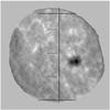 |
Fig. 1 The slit-jaw image recorded on October 21, 2010 with a 580 × 580 pixel CCD camera using an interference filter with 1.5 Å bandwidth centered on the Ca ii 3933 Å K line. The spot is in the NOAO region 1113 at W20N16. The dark vertical line represents the slit, the dark horizontal lines delimit the 0″ to 184″ spatial range imaged on the ZIMPOL sensor, and the spatial scale in arcsec is indicated. The slit is oriented such that it is parallel to the heliographic polar axis. |
The ZIMPOL technique is based on a fast modulation analyzer connected to a special demodulating CCD sensor on which three out of four pixel rows are masked. Shifting synchronously the collected photo-electron charges between the masked and unmasked pixel rows, one gets four intensity images corresponding to different modulation phase intervals. The Stokes images are obtained through linear combinations of these four images. Owing the high modulation frequency, seeing effects are effectively frozen and do not cause spurious polarization signatures in the fractional polarization images Q/I, U/I, and V/I (see Gandorfer & Povel 1997, for more details).
Since we used a single piezo-elastic modulator (working at 42 kHz), two separate measurements were required to obtain the full Stokes vector. The two measurements are carried out by rotating the analyzer (piezo-elastic modulator and linear polarizer) by 45°. In the first position, we obtain the Stokes I, Q/I, and V/I determinations, and in the second position I, U/I, and V/I. A sequence of 100 frames each exposed for 1 s are recorded at each position. In total, we recorded 5 or 10 sequences of 100 frames per position. The total time required for 10 sequences is about one hour.
With the help of an image rotator (a Dove prism), the solar image on the spectrograph slit plane is rotated to the desired orientation. The image rotation caused by the Gregory-Coudé telescope is compensated automatically. The polarization analyzer is positioned in front of the Dove prism and rotates accordingly.
The image on the spectrograph slit plane (slit jaw image) is re-imaged by a telecentric system on a CCD camera (Fig. 1). A 1.5 Å FWHM Daystar interference filter centered on the Ca ii K 3933 Å line is placed in front of the slit-jaw camera that allows us to locate the measured region on the Sun and to more clearly identify relevant structures in the selected region. Slit-jaw images are recorded every eight seconds to verify the accuracy of the tracking.
A typical observing run includes dark and flat field measurements as well as polarization calibrations, which are obtained with linear and circular polarizers that are inserted near the exit window of the telescope.
We cannot insert the calibration optics before this location. A glass tilt-plate, whose orientation is controlled by stepper motors, is inserted just after the calibration optics and allows us to compensate for the linear polarization that is caused by the telescope. The remaining instrumental polarization effects produced by the telescope are corrected for in the data reduction.
The position of the observed region is kept fixed on the spectrograph slit by the automatic guiding system (Küveler et al. 1998, 2010, 2011) which also compensates for the solar rotation. The position is held with a precision of 1''̣5 to 2″ (rms).
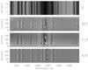 |
Fig. 2 Stokes images in a spectral window around the Ca i 4227 Å line. The observation was performed in the region shown in Fig. 1. Dark current and polarization calibration were taken into account, but not the instrumental cross talks between the Stokes parameters. In the Q/I and U/I images, the grey scale cuts are ±0.2%, while in the V/I image they are ±2.5%. |
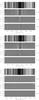 |
Fig. 3 Top observation: the same recording as in Fig. 2 after application of the cross-talk correction and of the linear polarization basis rotation (see text). The measurement was done around μ = 0.94. The second observation (middle) reports measurements of October 15 (around μ = 0.95) in the region shown in Fig. 5. The third observation was done on November 5 (bottom) very close to disk center (μ = 1) in a very quiet region. Here we note the absence of linear polarization signature. For all recordings, the grey scale cuts are the same as in Fig. 2. |
Figure 2 shows polarization images obtained on October 21, 2010 near the sunspot in NOAO region 1113. Dark recordings and polarization calibrations were taken into account, and spikes caused by cosmic rays or hot pixels have been removed by a software filter. Flat field and Fourier filter corrections were applied additionally. The corresponding slit position is shown in Fig. 1, with the slit oriented parallel to the heliographic polar axis. The center of the spectrograph slit is located at N17 W18. The spectral range covers 6.6 Å distributed over 1240 pixels (5.3 mÅ per pixel). In the spatial direction an angular extent of 184″ is covered by 140 (unmasked) pixel rows (thus effectively 1''̣3 per pixel). The typical statistical pixel noise in the polarization images is about 2 × 10⁻⁴.
The observations were carried out in October and November 2010 when the instrumental effects were no longer negligible, the main relevant source of troubles beeing the circular to linear polarization cross talk. The correction coefficients are extracted from the instrumental polarization measurements shown in Figs. 1 and 2 of 11.
Positive Q/I is defined as the amount of linear polarization along the spectrograph slit. To convert the Stokes images to the linear polarization basis used for the theoretical model (Anusha et al. 2011a), a basis transformation is needed. In the new basis, the positive Q/I direction is defined to be perpendicular to the local radius vector for each point along the spectrograph slit. The basis transformation thus has to be applied pixel by pixel along the slit, using the angle formed by the slit with the local radius vector. The top panel in Fig. 3 shows the results after these corrections.
3. Results
Among the observations obtained during this observing campaign, the results illustrated in the top and middle panels of Fig. 3 are typical of observations performed close to moderately active regions. We first consider the Q/I and U/I signatures in the Ca i 4227 Å line center.
As shown by 2, the observed amplitude of the linear polarization at line center is much too large to be explainable in terms of the transverse Zeeman effect, but can be interpreted and modeled in terms of the forward-scattering Hanle effect.
The observation of October 21 was performed rather close to disk center. The μ (= cosθ, where θ is the heliocentric angle) value varies along the slit from μ = 0.96 at coordinate 0″ to μ = 0.915 at coordinate 184″. Even at these quite large μ values, we can recognize weak features of about 3 × 10⁻⁴ in Q/I produced by scattering-polarization in the line wings around 4226.2 Å and 4227.1 Å, arising from the so called partial frequency redistribution mechanism in resonance scattering (see Anusha et al. 2011b).
The blend lines, most of them Fe i lines, show the usual Zeeman signatures caused by oriented magnetic fields in the layers where they are formed (see V/I profiles in the lower panels of Fig. 4).
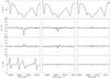 |
Fig. 4 Stokes spectra extracted from the observations in Fig. 3. Left panels: data of October 21 at coordinate 88″. Central panels data measured on October 15, around coordinate 25″. Right panels: Stokes profiles recorded in the very quiet region near disk center on November 5 around coordinate 52″. |
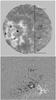 |
Fig. 5 Top panel: the slit jaw image of the region observed on October 15, 2010. Bottom panel: a 900″ × 700″ area of an MDI magnetogram recorded on October 15, 2010, approximately at the same time as our observation. Heliographic north is up. Grey scale cuts at ± 100 G are used. Overplotted is the position of the spectrograph slit. |
In Fig. 4, the Stokes profiles extracted from the Stokes images reported in Fig. 3 are presented. In the left panel, the profiles were averaged over four pixels, corresponding to 5''̣3 along the spatial direction, at slit coordinate 88″. The amplitudes of the linear polarization peaks in the left panels are among the largest that we found in our observing campaign. The largest degree of linear polarization that was recorded was about 0.75% (not shown here).
The central panels show Stokes profiles extracted from data measured on October 15, averaged over 12″ around coordinate 25″. Data measured in this region were analyzed by 2. The slit was placed near the active region NOAO 1112, as shown in the magnetogram in Fig. 5, for which the grey scale cuts are at ± 100 G. We can see that although the local photospheric magnetic field is faint at the slit position, the forward-scattering Hanle effect gives clear linear polarization signatures there.
The Stokes profiles in the right panels refer to the recording on November 5 done in a very quiet region near disk center, averaged over 9″ around coordinate 52″. The chosen portion of the slit represents the place with a detectable linear polarization signature. In really quiet regions far from (moderately) active regions, it is relatively rare to find polarization signatures that are significantly above the noise level.
To measure a significant forward-scattering signature, we need a magnetic field with a well defined azimuth direction within the resolution area observed (see for instance Fig. 1, in Trujillo Bueno 2001). The absence of signatures can be interpreted in terms of either turbulent magnetic structures, or very faint magnetic structures, or fast evolving structures in the observed area. As the total observation time per recording is of the order one hour, we average over effects such as temporal evolution and the local proper motions of the atmospheric structures. Nevertheless, the well-defined quality of the polarization signatures, and both their profile shapes and spatial distributions indicate that long-lived chromospheric magnetic structures with spatial scales of order 5″ exist, and that we can therefore use
this kind of data to diagnose chromospheric vector magnetic fields in the neighborhood of moderately active regions.
4. Conclusions
Our observations of the forward-scattering Hanle effects in the Ca i 4227 Å line has revealed many well-defined polarization signatures that could be reproduced with synthetic Stokes profiles computed with coherent scattering in one-dimensional semi-empirical models of the solar atmosphere (Anusha et al. 2011a). We recorded polarization profiles with amplitudes up to about 0.7% in the degree of linear polarization, which is much higher than can be explained in terms of the transverse Zeeman effect. The signal-to-noise ratio level of about 2 × 10⁻⁴ per pixel is reached in about one hour with a 45 cm aperture telescope. The richness of the profile shapes and the significant spatial variations on a scale of a few arcsec show that long-lived chromospheric magnetic structures are common. This together with the accompanying theoretical analysis of 2 demonstrates that the forward-scattering Hanle effect in the Ca i 4227 Å line is indeed a useful and important tool to measure the vector magnetic field (amplitude and orientation) in the low chromosphere near the center of the solar disk.
Acknowledgments
IRSOL is financed by Canton Ticino and the city of Locarno, together with the municipalities affiliated with CISL. The project has been supported by the Swiss Nationalfonds (SNF) grant 200020-127329. L.S.A. thanks the Indo-Swiss Joint Research Program (ISJRP) and IRSOL for supporting her visit to IRSOL. R.R. acknowledges the financial support provided by the foundation Carlo e Albina Cavargna. IRSOL acknowledges the financial support provided by the foundation Aldo e Cele Daccò. The ZIMPOL electronics is now developed at SUPSI under the direction of I. Defilippis. We are grateful to D. Gisler for his decisive help in the ZIMPOL project. The improved version of the Primary Image Guiding system has been developed at RheinMain University of Applied Sciences under the direction of G. Küveler. We are greateful to the anomymous referee for the useful suggestions.
References
- Anusha, L. S., Nagendra, K. N., Stenflo, J. O., et al. 2010, ApJ, 718, 988 [NASA ADS] [CrossRef] [Google Scholar]
- Anusha, L. S., Nagendra, K. N., Bianda, M., et al. 2011a, ApJ, submitted [Google Scholar]
- Anusha, L. S., Stenflo, J. O., Frisch, H., et al. 2011b, in Solar Polarization 6, ed. J. Kuhn et al., ASP Conf. Ser., 437, 57 [Google Scholar]
- Bianda, M., Ramelli, R., Trujillo Bueno, J., & Stenflo, J. O. 2006, in Solar Polarization 4, ASP Conf. Ser., 358, 454 [NASA ADS] [Google Scholar]
- Fontenla, J. M., Avrett, E. H., & Loeser, R. 1993, ApJ, 406, 319 [NASA ADS] [CrossRef] [Google Scholar]
- Joos, F. 2002, Master thesis, Institute of Astronomy, ETH Zurich [Google Scholar]
- Gandorfer, A. M., & Povel, H. P. 1997, A&A, 328, 381 [NASA ADS] [Google Scholar]
- Holzreuter, R., Fluri, D. M., & Stenflo, J. O. 2005, A&A, 434, 713 [NASA ADS] [CrossRef] [EDP Sciences] [Google Scholar]
- Küveler, G., Wiehr, E., Thomas, D., et al. 1998, Sol. Phys., 182, 247 [NASA ADS] [CrossRef] [Google Scholar]
- Küveler, G., Dao, V. D., Zuber, A., & Ramelli, R. 2010, Adv. Astron., Article ID 620424 [Google Scholar]
- Küveler, G., Dao, V. D., & Ramelli, R. 2011, Astron. Notes, in press [Google Scholar]
- Manso Sainz, R., Trujillo Bueno, J. 2010, ApJ, 722, 1416 [NASA ADS] [CrossRef] [Google Scholar]
- Ramelli, R., Bianda, M., Trujillo Bueno, J., Merenda, L., & Stenflo, J. O. 2005, in Proceedings of Chromospheric and Coronal Magnetic Fields, ed. D. E. Innes et al., ESA SP, 596, 82 [NASA ADS] [Google Scholar]
- Ramelli, R., Balemi, S., Bianda, M., et al. 2010, in Proc. SPIE 7735, ed. I. S. McLean et al., 77351Y-77351Y-12 [Google Scholar]
- Sampoorna, M., Stenflo, J. O., Nagendra, K. N., et al. 2009, ApJ, 699, 1650 [NASA ADS] [CrossRef] [Google Scholar]
- TrujilloBueno, J. 2001, in Advanced Solar Polarimetry – Theory, Observation, and Instrumentation, ed. M. Sigwarth, ASP Conf. Ser., 236, 161 [Google Scholar]
- Trujillo Bueno, J., Landi Degl’Innocenti, E., Collados, M., Merenda, L., & Manso Sainz, R. 2002, Nature, 415, 403 [NASA ADS] [CrossRef] [PubMed] [Google Scholar]
All Figures
|
Fig. 1 The slit-jaw image recorded on October 21, 2010 with a 580 × 580 pixel CCD camera using an interference filter with 1.5 Å bandwidth centered on the Ca ii 3933 Å K line. The spot is in the NOAO region 1113 at W20N16. The dark vertical line represents the slit, the dark horizontal lines delimit the 0″ to 184″ spatial range imaged on the ZIMPOL sensor, and the spatial scale in arcsec is indicated. The slit is oriented such that it is parallel to the heliographic polar axis. |
| In the text | |
|
Fig. 2 Stokes images in a spectral window around the Ca i 4227 Å line. The observation was performed in the region shown in Fig. 1. Dark current and polarization calibration were taken into account, but not the instrumental cross talks between the Stokes parameters. In the Q/I and U/I images, the grey scale cuts are ±0.2%, while in the V/I image they are ±2.5%. |
| In the text | |
|
Fig. 3 Top observation: the same recording as in Fig. 2 after application of the cross-talk correction and of the linear polarization basis rotation (see text). The measurement was done around μ = 0.94. The second observation (middle) reports measurements of October 15 (around μ = 0.95) in the region shown in Fig. 5. The third observation was done on November 5 (bottom) very close to disk center (μ = 1) in a very quiet region. Here we note the absence of linear polarization signature. For all recordings, the grey scale cuts are the same as in Fig. 2. |
| In the text | |
|
Fig. 4 Stokes spectra extracted from the observations in Fig. 3. Left panels: data of October 21 at coordinate 88″. Central panels data measured on October 15, around coordinate 25″. Right panels: Stokes profiles recorded in the very quiet region near disk center on November 5 around coordinate 52″. |
| In the text | |
|
Fig. 5 Top panel: the slit jaw image of the region observed on October 15, 2010. Bottom panel: a 900″ × 700″ area of an MDI magnetogram recorded on October 15, 2010, approximately at the same time as our observation. Heliographic north is up. Grey scale cuts at ± 100 G are used. Overplotted is the position of the spectrograph slit. |
| In the text | |
Current usage metrics show cumulative count of Article Views (full-text article views including HTML views, PDF and ePub downloads, according to the available data) and Abstracts Views on Vision4Press platform.
Data correspond to usage on the plateform after 2015. The current usage metrics is available 48-96 hours after online publication and is updated daily on week days.
Initial download of the metrics may take a while.