| Issue |
A&A
Volume 530, June 2011
|
|
|---|---|---|
| Article Number | A18 | |
| Number of page(s) | 12 | |
| Section | Atomic, molecular, and nuclear data | |
| DOI | https://doi.org/10.1051/0004-6361/201116511 | |
| Published online | 29 April 2011 | |
New effective recombination coefficients for nebular N ii lines⋆
1
Department of AstronomySchool of Physics, Peking University, Beijing 100871, PR China
e-mail: This email address is being protected from spambots. You need JavaScript enabled to view it.
2
Department of Physics and Astronomy, University College London, Gower Street, London WC1E 6BT, UK
3
The Kavli Institute for Astronomy and Astrophysics, Peking University, Beijing 100871, PR China
Received: 14 January 2011
Accepted: 22 March 2011
Abstract
Aims. In nebular astrophysics, there has been a long-standing dichotomy in plasma diagnostics between abundance determinations using the traditional method based on collisionally excited lines (CELs), on the one hand, and (optical) recombination lines/continuum, on the other. A number of mechanisms have been proposed to explain the dichotomy. Deep spectroscopy and recombination line analysis of emission line nebulae (planetary nebulae and H ii regions) in the past decade have pointed to the existence of another previously unknown component of cold, H-deficient material as the culprit. Better constraints are needed on the physical conditions (electron temperature and density), chemical composition, mass, and spatial distribution of the postulated H-deficient inclusions in order to unravel their astrophysical origins. This requires knowledge of the relevant atomic parameters, most importantly the effective recombination coefficients of abundant heavy element ions such as C ii, O ii, N ii, and Ne ii, appropriate for the physical conditions prevailing in those cold inclusions (e.g. Te ≤ 1000 K).
Methods. Here we report new ab initio calculations of the effective recombination coefficients for the N ii recombination spectrum. We have taken into account the density dependence of the coefficients arising from the relative populations of the fine-structure levels of the ground term of the recombining ion (2P° 1/2 and 2P° 3/2 in the case of N iii), an elaboration that has not been attempted before for this ion, and it opens up the possibility of electron density determination via recombination line analysis. Photoionization cross-sections, bound state energies, and the oscillator strengths of N ii with n ≤ 11 and l ≤ 4 have been obtained using the close-coupling R-matrix method in the intermediate coupling scheme. Photoionization data were computed that accurately map out the near-threshold resonances and were used to derive recombination coefficients, including radiative and dielectronic recombination. Also new is including the effects of dielectronic recombination via high-n resonances lying between the 2P° 1/2 and 2P° 3/2 levels. The new calculations are valid for temperatures down to an unprecedentedly low level (approximately 100 K). The newly calculated effective recombination coefficients allow us to construct plasma diagnostics based on the measured strengths of the N ii optical recombination lines (ORLs).
Results. The derived effective recombination coefficients are fitted with analytic formulae as a function of electron temperature for different electron densities. The dependence of the emissivities of the strongest transitions of N ii on electron density and temperature is illustrated. Potential applications of the current data to electron density and temperature diagnostics for photoionized gaseous nebulae are discussed. We also present a method of determining electron temperature and density simultaneously.
Key words: atomic data / line: formation / Hii regions / ISM: atoms / planetary nebulae: general
Tables 3–15 are only available at the CDS via anonymous ftp to cdsarc.u-strasbg.fr (130.79.128.5) or via http://cdsarc.u-strasbg.fr/viz-bin/qcat?J/A+A/530/A18
© ESO, 2011
1. Introduction
The principal means of electron temperature and density diagnostics and heavy-element abundance determinations in nebular plasmas has, until recently, been measurement of collisionally excited lines (CELs). The emissivities of CELs have, however, an exponential dependence on electron temperature and, consequently, so do the heavy element abundances deduced from them. An alternative method of determining heavy element abundances is to divide the intensities of ORLs emitted by heavy element ions with those by hydrogen. Such ratios are only weakly dependent on temperature. In planetary nebulae (PNe), abundances of C, N, and O derived from ORLs have been shown to be systematically larger than those derived from CELs typically by a factor of 2. Discrepancies of much larger magnitudes, say by more than a factor of 5, are also found for a small fraction of PNe (about 10%; Liu et al. 1995, 2000, 2001, 2006b, 2004; Luo et al. 2001). In the most extreme case, the abundance discrepancy factor (ADF) reaches a record value of 70 (Liu et al. 2006). There is strong evidence that nebulae contain another component of metal-rich, cold plasma, probably in the form of H -deficient inclusions embedded in the diffuse gas (Liu et al. 2000). The existence of cold inclusions provides a natural explanation to the long-standing dichotomy of abundance determinations and plasma diagnostics (Liu 2003, 2006a,b). The prerequisite for reliable determinations of recombination line abundances is accurate effective recombination coefficients for heavy element recombination lines. In this paper, we present new effective recombination coefficients for the recombination spectrum of N ii.
Radiative recombination coefficients of N ii have been given by Péquignot et al. (1991). Nussbaumer & Storey (1984) tabulate dielectronic recombination coefficients of N ii obtained from a model in which resonance states are represented by bound-state wave functions. Escalante & Victor (1990) calculate effective recombination coefficients for C i and N ii lines using an atomic model potential approximation for transition probabilities and recombination cross-sections. They then add the contribution from dielectronic recombination using the results of Nussbaumer & Storey (1984).
In the most recent work of N ii by Kisielius & Storey (2002), they follow the approach of Storey (1994) who, in dealing with O ii, uses a unified method for the treatment of radiative and dielectronic recombination by directly calculating recombination coefficients from photoionization cross-sections of each initial state. They also incorporate improvements introduced by Kisielius et al. (1998) in their work on Ne ii. The N+ photoionization cross-sections were calculated in LS-coupling using the ab initio methods developed for the Opacity Project (Seaton 1987; Berrington et al. 1987) and the Iron Project (Hummer et al. 1993), hereafter referred to as the OP methods. The calculations employed the R-matrix formulation of the close-coupling method, and the resultant cross-sections are of higher quality. In the photoionization calculations of Kisielius & Storey (2002), for the energy ranges in which the resonances make main contributions to the total recombination, an adaptive energy mesh was used to map out all the strong resonances near thresholds. This approach has also been adopted in our current calculations, and it will be described in more details in a later section. In the work of Kisielius & Storey (2002), transition probabilities for all low-lying bound states were also calculated using the close-coupling method, so that the bound-bound and bound-free radiative data used for calculating the recombination coefficients formed a self-consistent set of data and were expected to be significantly more accurate than those employed in earlier work.
Here we report new calculations of the effective recombination coefficients for the N ii recombination spectrum. Hitherto few high quality atomic data were available to diagnose plasmas of very low temperatures ( ≤ 1000 K), such as the cold, H-deficient inclusions postulated to exist in PNe (Liu et al. 2000). We have calculated the effective recombination coefficients for the N+ ion down to an unprecedentedly low temperature (about 100 K). At such low temperatures, dielectronic recombination via high-n resonances between the N2+ ground 2P° 1/2 and 2P° 3/2 fine-structure levels contributes significantly to the total recombination coefficient. We include such effects in our calculations. We also take into account the density dependence of the coefficients through the level populations of the fine-structure levels of the ground state of the recombining ion (2P° 1/2,3/2 in the case of N2+). That opens up the possibility of electron density determinations via recombination line analysis. With the exception of the calculations of Kisielius & Storey (1999) on O iii recombination lines, all previous work on nebular recombination lines has been in LS-coupling and therefore it tacitly assumed that the levels of the ground state are populated in proportion to their statistical weights. Photoionization cross-sections, bound state energies and oscillator strengths of N ii with n ≤ 11 and l ≤ 4 have been obtained using the R-matrix method in the intermediate coupling scheme. The photoionization data are used to derive recombination coefficients, including contributions from radiative and dielectronic recombination. The results are applicable to PNe, H ii regions and nova shells for a wide range of electron temperature and density.
2. Atomic data for N+
2.1. The N+ term scheme
The principal series of N ii is 2s22p(2P°)nl, which gives rise to singlet and triplet terms. Also interspersed are members of the series 2s2p2(4P)nl (n = 3, 4) giving rise to triplet and quintet terms. Higher members of this series lie above the first ionization limit, and hence may give rise to low-temperature dielectronic recombination. There are a few members of the 2s2p2(2D)nl and 2s2p2(2S)nl series located above the first ionization threshold which also give rise to resonance structures in the photoionization cross-sections for singlets and triplets. For photon energies above the second ionization threshold, the main resonance structures are due to the 2s2p2(2D)nl series with some interlopers from the 2s2p2(2S)nl and 2s2p2(2P)nl series (Kisielius & Storey 2002).
2.2. New R-matrix calculation
We have carried out a new calculation of bound state energies, oscillator strengths and photoionization cross-sections for N ii states with n ≤ 11 using the OP methods (Hummer et al. 1993). The N2+ target configuration set was generated with the general purpose atomic structure code SUPERSTRUCTURE (Eissner et al. 1974) with modifications of Nussbaumer & Storey (1978). The target radial wave functions of N2+ were then generated with another atomic structure code AUTOSTRUCTURE1, which, developed from SUPERSTRUCTURE and capable of treating collisions, is able to calculate autoionization rates, photoionization cross-sections, etc. The original theory of AUTOSTRUCTURE is described by Badnell (1986). The wave functions of the nineteen target terms were expanded in terms of the 21 electron configurations 1s22s22p, 1s22s2p2, 1s22p3, 1s22s s, 1s22sp, 1s22sd, 1s22s2p
 s, 1s22s2pp, 1s22s2pd, 1s22ps, 1s22pp, 1s22pd, 1s22sd2, 1s22pd2, 1s22s
 s, 1s22sd, 1s22s2p
 s, 1s22s2pp, 1s22s2pd, 1s22s2pf, 1s22pp, where 1s, 2s and 2p are spectroscopic orbitals and
  and
and  (l = 0 − 2 and l′ = 0 − 3) are correlation orbitals. The one-electron radial functions for the 1s, 2s and 2p orbitals were calculated in adjustable Thomas-Fermi potentials, while the radial functions for the remaining orbitals were calculated in Coulomb potentials of variable nuclear charge, Znl = 7 | λnl | . The potential scaling parameters λnl were determined by minimizing the sum of the energies of the eight energetically lowest target states in our model. We obtained for the potential scaling parameters: λ1s = 1.4279, λ2s = 1.2840, λ2p = 1.1818,
  ,
,  ,
,  ,
,  ,
,  ,
,  and
and  .
.
Comparison of energies (in Ry) for the N2+ target states.
The N2+ target terms.
In Table 1, we compare experimental target state energies (Eriksson 1983) as well as values calculated by Kisielius & Storey (2002) with our results for the eight lowest target terms that belong to the three lowest configurations, 2s22p, 2s2p2 and 2p3. We use the experimental target energies in the calculation of the Hamiltonian matrix of the (N + 1) electron system and in the calculation of energy levels, oscillator strengths and photoionization cross-sections of N ii. We use nineteen target terms in our R-matrix calculation where we add selected terms from the seven configurations 1s22s s, 1s22sp, 1s22sd, 1s22s2p s, 1s22s2p p, 1s22s2p d and 1s22p2
  in order to increase the dipole polarizability of the terms of the 2s22p and 2s2p2 configurations of the N2+ target. These additional terms provide the main contributions to the dipole polarizability of the 1s22s22p 2P° and 1s22s2p2 4P states and significant contributions to the polarizability of 1s22s2p2 2D, 2S and 2P. The chosen target terms are listed in Table 2, which shows that our calculated target energies are in slightly worse agreement with experiment than those of Kisielius & Storey (2002) although it should be noted that their energies were calculated in LS-coupling, whereas ours are weighted averages of fine-structure level energies. The configuration interaction in our target is less extensive than in theirs due to the additional computational constraints imposed by an intermediate coupling calculation as opposed to an LS-coupling one. We do, however, consider that our set of target states represents the polarizability of the important N2+ states better than does the target of Kisielius & Storey (2002).
2.3. Energy levels of N+
Experimental energy levels for N+ have been given by Eriksson (1983) for members of the series 2s22p(2P°) nl with n ≤ 16 and l ≤ 4, for the series 2s2p2(4Pe) nl with n ≤ 12 and l ≤ 4 and for the series 2s2p2(2De) 3l, 4p although some levels are missing. Energy levels for the states 3Pe2,1,0 belonging to the equivalent electron configuration 2s22p4 are also presented. We use these experimental data as a benchmark for our N ii energy level calculation.
The current calculations of energy levels include only the states belonging to the configurations 2s22p(2P ) nl, 2s2p2(4P
 ) nl and possibly 2s2p2(2D) nl with ionization energies less than E0 (corresponding to n = 11 in the principal series of N ii) and total orbital angular momentum quantum number L ≤ 8, where JC is the total angular momentum quantum number of the core electrons. Every single energy level calculated by ab initio methods is further identified with the help of the experimental energy level tables of Eriksson (1983), and is used in preference to quantum defect extrapolation from experimentally known lower states. The bound state energies for the lowest levels are calculated using R-matrix codes, with an effective principal quantum number range set to be 0.5 ≤ ν ≤ 10.5, and the codes are run with a searching step of δν = 0.01. We assume that the subsequent iteration converges on a final energy when Δ E < 1 × 10⁻⁵ Ryd. We only keep the final energy levels with n ≤ 11 and l ≤ 4, and delete the ng levels with n > 6, because of numerical instabilities in the codes. In total, 377 levels are obtained. The photoionization cross-sections from these bound states are calculated later using outer region R-matrix codes.
For states with 11 < n ≤ nd, and l ≤ 3, where calculated energies exist for lower members of the series, a quantum defect has been calculated for the highest known member (usually with n = 11), and this quantum defect is used to determine the energies of all higher terms.
Finally, if neither of the above methods can be used, the state is assumed to have a zero quantum defect.
2.4. Bound-bound radiative data
Radiative transition probabilities are taken from three sources,
-
(1)
Ab initio calculations: we have computed values of weightedoscillator strengths, gf, for all transitions between bound states with ionization energies less than or equal to E0 (corresponding to n = 11 in the principal series of N+), with total orbital angular momentum quantum number L ≤ 8, and with total angular momentum quantum number J ≤ 6. The data are calculated in the intermediate coupling scheme, so there are transitions between states of different total spins. Two-electron transitions, which involve a change of core state, are also included.
-
(2)
Coulomb approximation: for pairs of levels where oscillator strengths are not computed by the ab initio method, but where one or both of the states have a non-zero quantum defect, the dipole radial integrals required for the calculation of transition probabilities are calculated using the Coulomb approximation. Details are given by Storey (1994).
-
(3)
Hydrogenic approximation: for pairs of levels with a zero quantum defect hydrogenic dipole radial integrals are calculated, using direct recursion on the matrix elements themselves as described by Storey & Hummmer (1991).
2.5. Photoionization cross-sections and recombination coefficients
The recombination coefficient for each level nls L [K] π J is calculated directly from the photoionization cross-sections for that state. There are three approximations in which the photoionization data are obtained.
-
(1)
Photoionization cross-sections are computed for all the377 states with ionization energy less than or equalto E0, L ≤ 8 and J ≤ 6. We obtain the recombination coefficient directly by integrating the appropriate R-matrix photoionization cross-sections.
-
(2)
Coulomb approximation: as in the bound-bound case, the Coulomb approximation is used for states where no OP data are available, but which have a non-zero quantum defect. The calculation of photoionization data using Coulomb functions has been described by Burgess & Seaton (1960) and Peach (1967).
-
(3)
For all states for which the R-matrix photoionization cross-sections have not been calculated explicitly, the hydrogenic approximation to the photoionization cross-sections is evaluated, using the routines of Storey & Hummer (1991) to generate radiative data in hydrogenic systems.
2.6. Energy mesh for N ii photoionization cross-sections
The photoionization cross-sections for N ii generated by the Opacity Project (OP) method were based on a quantum defect mesh with 100 points per unit increase in the effective quantum number derived from the next threshold. In contrast to the OP calculations, we use a variable step mesh for photoionization cross-section calculations for a particular energy region above the 2P° 3/2 threshold, which is appropriate to dielectronic recombination in nebular physical conditions. This energy mesh delineates all resonances to a prescribed accuracy (Kisielius et al. 1998; Kisielius & Storey 2002). This detailed consideration of the energy mesh was undertaken for the region from the 2s22p (2P° 3/2) limit up to 0.160 Ryd (n = 5) below the 2s2p2 (4P 1/2) limit, since this region contains the main contribution to the total recombination at the temperatures of interest for the triplet and singlet series.
From 0.160 Ryd below the 2s2p2 (4P 1/2) limit to 0.0331 Ryd below the 2s2p2 (4P 1/2) limit, we use a quantum defect mesh with an increment of 0.01 in effective principal quantum number. The energy 0.160 Ryd corresponds to a principal quantum number of five relative to the next threshold, and 0.0331 Ryd corresponds to eleven. In total about 600 points are used in this region. For the region from 0.0331 Ryd (n = 11) below the 2s2p2 (4P 1/2) limit up to the 2s2p2 (4P 5/2) limit, we use the Gailitis average (Gailitis 1963). We use the method for this part of photoionization calculations because of the very dense resonances in this narrow energy region. About 100 points are used.
In the region from the 2s2p2 (4P 5/2) limit up to 0.0331 Ryd (n = 11) below the 2s2p2 (2D 3/2) limit, a quantum defect mesh is again used, with an increment of 0.01 in effective principal quantum number. Here 0.0331 Ryd corresponds to a principal quantum number of eleven relative to the next threshold, 2s2p2 (2D 3/2). There are about 800 points used in this region. For the energetically lowest region between the two ground fine-structure levels of N iii, 2s22p (2P° 1/2) and 2s22p (2P° 3/2), we use linear extrapolation from a few points lying right above the 2s22p (2P° 3/2) threshold. About 100 points are used in this region.
During the calculation of photoionization cross-sections, we check for every bound states to make sure that the cross-section data of different energy areas all join smoothly. Figure 1 shows the photoionization cross-sections calculated from the five lowest levels 3Pe 0, 3Pe 1, 3Pe 2, 1De 2 and 1Se 0 belonging to the ground configuration 1s22s22p2 of N+. Photoionization cross-sections calculated for the five different energy regions have been joined together.
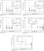 |
Fig. 1 The data calculated by different methods for the five energy regions have been joined together. The insert zooms in a particular energy area, and the mesh points used for the photoionization calculations are shown in the inset. |
3. Calculation of N+ population
3.1. The N+ populations
The calculation of populations is a three stage process to compute departure coefficients, b(JC;nl K J), defined in terms of populations by 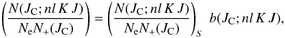 (1)where JC is an N2 + core state and the subscript S refers to the value of the ratio given by the Saha and Boltzmann equations, and Ne and N + (JC) are the number densities of electrons and recombining ions, respectively. We distinguish two boundaries in principal quantum number, nd and nl. For n ≤ nd collisional processes are negligible compared to radiative decays and can be omitted from the calculation of the populations. For higher n a full collisional-radiative treatment of the populations is necessary as described by Hummer & Storey (1987) and Storey & Hummer (1995) with some additions to treat dielectronic recombination. The boundary at n = nl is defined such that for n > nl the redistribution of population due to l-changing collisions is rapid enough to assume that the populations obey the Boltzmann distribution for a given n and hence that bnl = bn for all l.
The three stages of the calculation are as follows:
-
Stage 1:
a calculation ofb(JC;n) is made for all n < 1000, using the techniques and atomic rate coefficients described by Hummer & Storey (1987) and Storey & Hummer (1995) with the addition of l-averaged autoionization and dielectronic capture rates computed with AUTOSTRUCTURE for states of (2P° 3/2) parentage that lie above the ionization limit. For n > 1000, we assume bn = 1. The results of this calculation provide the values of b for n > nl and the initial values for n ≤ nl for Stage 2.
-
Stage 2:
a calculation of b(JC;nl K J) is made for all n ≤ nl using the same collisional-radiative treatment as in Stage 1 but now resolved by total J. The combined results of Stages 1 and 2 provide the values of b for n > nd.
-
Stage 3:
for the energies less than that which corresponds to n = nd in the principal series, departure coefficients b(JC;nl K J) are computed for states of all series. Since only spontaneous radiative decays link these states, the populations are obtained by a step-wise solution from the energetically highest to the lowest state.
3.2. Dielectronic recombination within the 2P° parents
Within the 2P° parents, the contribution by dielectronic recombination to the total recombination is shown to become significant at very low temperatures ( ≤ 250 K), due to recombination into high-lying bound states of the 2P parent from the 2P
 continuum states. We incorporate this low-temperature process into our calculation of the N+ populations. Figure 2 is a schematic diagram illustrating N ii dielectronic capture, autoionization and radiative decays. The electrons captured to the high-n autoionizing levels decay to low-n bound states through cascades, and optical recombination lines are emitted. Radiative transitions which change parent, such as (2P)n1l1–(2P)n0l0, are included for those states for which R-matrix calculated values are present. Higher states are treated by hydrogenic or Coulomb approximations which do not allow parent changing transitions.
In Fig. 2, three multiplets of N ii are presented as examples: V3 2s22p3p 3De–2s22p3s 3P°, the strongest 3p–3s transition, V19 2s22p3d 3F°–2s22p3p 3De, the strongest 3d–3p transition, and V39 2s22p4f G[7/2,9/2]e–2s22p3d 3F°, the strongest 4f − 3d transition. The results for these three multiplets are analysed in Sect. 4.3.
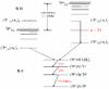 |
Fig. 2 Schematic figure showing the low-temperature ( ≤ 250 K) dielectronic recombination of N ii through the fine-structure autoionizing levels between the two lowest ionization thresholds of N iii 2P° 1/2 and 2P° 3/2. The electrons captured to the high-n autoionizing levels decay to low-n bound states through cascades and optical recombination lines (ORLs) are thus emitted. Here Multiplets V3, V19 and V39 are presented as examples. |
3.3. The 2P° parent populations
The contribution to the total recombination coefficient of a state depends on the relative populations of the 2P° 1/2 and 2P° 3/2 parent levels, which generally dominate the populations of the recombining ion N2+ under typical nebular physical conditions. The relative populations of the two fine-structure levels deviate from the statistical weight ratio, 1:2, which is assumed in all work hitherto on this ion. The deviation affects the populations of the high Rydberg states, and consequently total dielectronic recombination coefficients at low-density and low-temperature conditions.
We model the N2+ populations with a five level atom comprising the two levels of the 2P° term and the three levels of the 4P term, although it should be noted that the populations of the three 4P levels are almost negligible in the nebular conditions considered here (Sect. 4.5). The relative populations are assumed to be determined only by collisional excitation, collisional de-excitation and spontaneous radiative decay. Transition probabilities were taken from Fang et al. (1993) and thermally averaged collision strengths from Nussbaumer & Storey (1979) and Butler & Storey (priv. comm.).
Figure 3 shows the fractional populations of the N2+ 2P and 2P
 fine-structure levels at several electron temperatures and as a function of electron density, ranging from 102 to 106 cm-3, applicable to PNe and H ii regions. The fractional populations vary significantly below 104 cm-3 and converge to the thermalized values at higher densities.
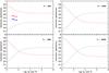 |
Fig. 3 Fractional populations of the N2+ 2P |
3.4. The Cases A and B
Baker & Menzel (1938) define the Cases A and B with reference to the recombination spectrum of hydrogen. In N ii, there are five low-lying levels belonging to the ground configuration 2s22p2, 3Pe 0,1,2, 1De 2 and 1Se 0. Just as in Kisielius & Storey (2002), we define two cases for N ii. In Case A, all emission lines are assumed to be optically thin. In Case B, lines terminating on the three lowest levels 3Pe 0,1,2 are assumed to be optically thick and no radiative decays to these levels are permitted when calculating the population structure. The latter case is generally a better approximation for most nebulae.
4. Results and discussion
4.1. Effective recombination coefficients
The population structure of N+ has been calculated for electron temperature log Te [K] = 2.1 ~ 4.3, with a step of 0.1 in logarithm, and for the electron density Ne = 102 ~ 106 cm-3, also with a step of 0.1 in logarithm. Constrained by the range of the exponential factors involved in the calculation of the departure coefficients using the Saha-Boltzmann equation, calculation of the effective recombination coefficients starts from 125 K (log Te = 2.1). For electron densities greater than 106 cm-3, as pointed out by Kisielius & Storey (2002), it is necessary to include l-changing collisions for n < 11. This is however beyond the scope of the current treatment.
In Tables 3−6 we present the effective recombination coefficient, αeff(λ), in units of cm3 s-1, for strongest N ii transitions with valence electron orbital angular momentum quantum number l ≤ 5, at electron densities Ne = 102, 103, 104 and 105 cm-3, respectively, in Case B. The effective recombination coefficient is defined such that the emissivity ϵ(λ), in a transition of wavelength λ is given by ![Mathematical equation: \begin{equation} \epsilon(\lambda) = N_{\rm e} N_+ \alpha_{\rm eff}(\lambda) {{hc}\over{\lambda}} \; \; \; \; [\rm{erg~cm}^{-3}~{\rm s}^{-1}]. \label{emissivity} \end{equation}](/articles/aa/full_html/2011/06/aa16511-11/aa16511-11-eq133.png) (2)Transitions included in the tables are selected according to the following criteria:
(2)Transitions included in the tables are selected according to the following criteria:
-
(1)
λ ≥ 912 Å;
-
(2)
αeff(λ) ≥ 1.0 × 10⁻¹⁴ cm3 s-1 at Te = 1000 K for all Ne’s, and ≥ 1.0 × 10⁻¹⁵ cm3 s-1 at all Te’s and Ne’s;
-
(3)
all fine-structure components are presented for multiplets from the 3d − 3p and 3p − 3s configurations. For the 4f − 3d configurations, a few selected multiplets are listed, but only V38 and V39 includes all the individual components. These transitions fall in the visible part of the spectrum and among them are the strongest recombination lines of N ii.
In Tables 3−6, the wavelengths of all the 4−3 and 3−3 transitions and majority of the 5−4 and 5−3 transitions are experimentally known. All the wavelengths of the 6−5 and 6−4 transitions are predicted. Our calculated wavelengths, derived from the experimental energies, agree with the experimentally known wavelengths within 0.001%. Our predicted wavelengths for experimentally unknown transitions agree with those predicted by Hirata & Horaguchi (1995) within 0.007% except for one 6d−3p transition wavelength which differs by 0.24 Å. However, this transition is spectroscopically less important compared to the 4−3 and 3−3 ones.
In these tables, we use the pair-coupling notation ![Mathematical equation: \hbox{$L[K]^{\pi}_{J}$}](/articles/aa/full_html/2011/06/aa16511-11/aa16511-11-eq149.png) for the states belonging to the (2P°) nf and ng configurations, as in Eriksson (1983). As shown by Cowan (1981), pair-coupling is probably appropriate for the states of intermediate-l (l = 3,4). The same notation is adopted for the (2P°) nh configurations. For states belonging to low-l (l ≤ 2) configurations, LS-coupling notation
for the states belonging to the (2P°) nf and ng configurations, as in Eriksson (1983). As shown by Cowan (1981), pair-coupling is probably appropriate for the states of intermediate-l (l = 3,4). The same notation is adopted for the (2P°) nh configurations. For states belonging to low-l (l ≤ 2) configurations, LS-coupling notation  is used.
4.2. Effective recombination coefficient fits
We fit the effective recombination coefficients as a function of electron temperature in logarithmic space with analytical expressions for selected transitions, using a non-linear least-square algorithm. Tables 7−14 present fit parameters and maximum deviations δ[%] for four densities, Ne = 102, 103, 104 and 105 cm-3. Only strongest optical transitions are presented, including multiplets V3, V5, V19, V20, V28, V29, V38 and V39. As the dependence of recombination coefficient on Te at electron temperatures below 10 000 K is different from that at high temperatures (10 000 ~ 20 000 K in our case), we use different expressions for the two temperature regimes.
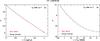 |
Fig. 4 Analysis fit to the effective recombination coefficients for the N ii V3 3p 3D3–3s 3P |
For the low-temperature regime, Te < 10 000 K, effective recombination coefficients are dominated by contribution from radiative recombination αrad, which has a relatively simple dependence on electron temperature, αrad ∝ Te−a, where a ~ 1. At low temperatures, dielectronic recombination through low-lying autoionizing states are also important for ions such as C ii, N ii, O ii, Ne ii (Storey 1981, 1983; Nussbaumer & Storey 1983, 1984, 1986, 1987). Considering the fact that direct radiative recombination rate is nearly a linear function of temperature in logarithm, and the deviation introduced by dielectronic recombination, we use a five-order polynomial expression to fit the effective recombination coefficient,  (3)where α = log 10 αeff + 15 and t = log 10 Te, and a0, a1, a2, a3, a4 and a5 are constants.
For the high-temperature regime, 10 000 ≤ Te ≤ 20 000 K, the contribution from dielectronic recombination, αDR, can significantly exceed that of direct radiative recombination (Burgess 1964). Dielectronic recombination coefficient αDR has a complex exponential dependence on Te (Seaton & Storey 1976; Storey 1981), αDR ∝  exp( − E/k Te), where E is the excitation energy of an autoionizing state, to which a free electron is captured, relative to the ground state of the recombining ion (N2+ in our case) and k is the Boltzmann constant. The expression adopted for this temperature regime is,
  (4)where α = log 10 αeff + 15 and t = Te [K] /104, the reduced electron temperature, and b0, b1, b2, b3, b4, b5 and b6 are constants.
In order to make the data fits accurate for the high-temperature regime, 10 000 ≤ Te ≤ 20 000 K, where the original calculations are carried out for only four temperature cases (log Te [K] = 4.0, 4.1, 4.2 and 4.3), nine more temperature cases are calculated. For the temperature region log Te [K] = 3.9 ~ 4.0, two more temperature cases are also calculated, so that the data fits near 10 000 K are accurate enough. Figure 4 is an example of the fit to the effective recombination coefficients of the N ii V3 2s22p3p 3D –2s22p3s 3P
 λ5679.56 transition.
By using different expressions for the two temperature regimes, we manage to control the maximum fitting errors to well within 0.5 per cent.
4.3. Relative intensities within N ii multiplets
As mentioned in the Sect. 3.4 above, the populations of the ground fine-structure levels 2P° 1/2,3/2 of the recombining ion N2+ vary with electron density under typical nebular conditions. The variations are reflected in the relative intensities of the resultant recombination lines of N ii, which arise from upper levels with the same orbital angular momentum quantum number l but of different parentage, i.e., 2P° 1/2 and 2P° 3/2 in the current case. A number of such recombination lines have been observed in photoionized gaseous nebulae including PNe and H ii regions, and their intensity ratios can thus be used for density diagnostics.
As the relative populations of 2P° 1/2,3/2 vary with Ne, so do the fractional intensities of individual fine-structure components within a given multiplet of N ii. The most prominent N ii multiplets in the optical include: V3 2s22p3p 3De–2s22p3s 3P°, V19 2s22p3d 3F°–2s22p3p 3De and V39 2s22p4f G[7/2,9/2]e–2s22p3d 3F°.
4.3.1. 2s22p3p 3De–2s22p3s 3P° (V3)
The fractional intensities of fine-structure components of Multiplet V3, 2s22p3p 3De–2s22p3s 3P°, are presented in Fig. 5. The strongest component is λ5679.56, which forms from core 2P° 3/2 capturing an electron plus cascades from higher states, while the second strongest component λ5666.63 can form, in addition, from recombination of core 2P° 1/2.
For the target N iii, the population of the fine-structure level 2P° 3/2 relative to 2P° 1/2 increases with electron density Ne due to collisional excitation, and consequently, so does the intensity of the λ5679.56 line relative to the λ5666.63 line. Their intensity ratio peaks around Ne = 2000 cm-3, the critical density Nc of the level 2P° 3/2, and then decreases as Ne increases further. The relative intensities of all components converge to constant values at high densities ( ≥ 105 − 106 cm-3), as the relative populations of the ground fine-structure levels of the target N iii approach the Boltzmann distribution.
The line ratio I(λ5679.56)/I(λ5666.63) thus serves as a density diagnostic for nebulae of low and intermediate densities, Ne ≤ 105 cm-3. At very low electron temperatures, where kTe is comparable to the 2P° 1/2–2P° 3/2 energy separation, the sensitivity to density in the components of V3 is reduced. This arises because, at very low temperatures, the states (2Po 3/2) nl are populated more significantly by dielectronic capture from the (2P° 1/2) κl continuum than by direct recombination on N2+ (2P° 3/2). The density dependence of the population distribution between the 2P° 1/2 and 2P° 3/2 is then of less importance.
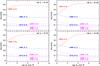 |
Fig. 5 Fractional intensities of components of Multiplet V3: 2s22p3p 3De–2s22p3s 3P°. The numbers in brackets following the wavelength labels are the total angular momentum quantum numbers J2 − J1 of the upper to lower levels of the transition. Components from upper levels of the same total angular momentum quantum number J are represented by same colour and line type. Four temperature cases, log 10Te = 2.5, 3.0, 3.5 and 4.0 K, are presented. |
4.3.2. 2s22p3d 3F°–2s22p3p 3De (V19)
The fractional intensities of fine-structure components of Multiplet V19, 2s22p3d 3F°–2s22p3p 3De, are presented in Fig. 6. The strongest component, λ5005.15, forms exclusively from recombination of target 2P° 3/2 plus cascades, while the second and third strongest components of almost identical wavelengths, λ5001.48 and λ5001.14, can form, in addition, from recombination of the ground target 2P° 1/2.
At very low densities of about 102 cm-3, 2P° 1/2 dominates the population of N iii, and this is manifested by the intensity of the λ5005.15 line being lower than the λ5001.48 line and than λ5001.14 by a further amount. As electron density increases, the intensity of the λ5005.15 line relative to the λ5005.48/15 lines increases and peaks around 2000 cm-3. At densities above 105 cm-3, the fractional populations of all components converge to constant values. The trends are similar to Multiplet V3 discussed above.
The intensity ratio I(λ5005.15)/I(λ5001.48 + λ5001.14) serves as another potential density diagnostic. In reality, however, given the closeness in wavelength of the λ5005.15 line to the [O iii] λ5007 nebular line, which is often several orders of magnitude (3 − 4) brighter, accurate measurement of λ5005.15 line is essentially impossible.
4.3.3. 2s22p4f G[7/2,9/2]e–2s22p3d 3F° (V39)
The fractional intensities of fine-structure components of Multiplet V39, 2s22p4f G[7/2,9/2]e–2s22p3d 3F°, are presented in Fig. 7. The strongest component λ4041.31 forms exclusively from recombination of target 2P° 3/2 plus cascades from higher states, while the second and third strongest components, λ4035.08 and λ4043.53, which have comparable intensities, can form, in addition, from recombination of target 2P° 1/2.
The behaviour of the intensity of the λ4041.31 line relative to those of the λ4035.08 and λ4043.53 lines as a function of electron density is quite similar to those of their counterparts of Multiplets V3 and V19 discussed above.
The line ratios I(λ4041.31)/I(λ4035.08) and I(λ4041.31)/ I(λ4043.53) can in principle serve as additional density diagnostics. There are however complications in their applications:
-
(1)
All fine-structure components of Multiplet V39 2s22p4f G[7/2,9/2]e–2s22p3d 3F° are extremely faint. The strongest component λ4041.31 is 2 − 3 times fainter than λ5679.56, the strongest component of V3, while the latter is typically one thousand times fainter than Hβ in a real nebula.
-
(2)
The λ4041.31 line is blended with the O ii recombination line λ4041.29 of Multiplet V50c 2p24f F[2]° 5/2–2p23d 4Fe 5/2, while the λ4035.08 line is blended with the O ii lines λ4035.07 of Multiplet V50b 2p24f F[3]° 5/2–2p23d 4Fe 5/2 and λ4035.49 of Multiplet V50b 2p24f F[3]° 7/2–2p23d 4Fe 5/2.
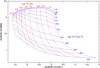 |
Fig. 8 Loci of the N ii recombination line ratios I(λ5679.56)/I(λ5666.63) and I(λ5679.56)/I(λ4041.31) for different Te’s and Ne’s. |
4.4. Plasma diagnostics
Unlike the UV and optical CELs, whose emissivities have an exponential dependence on Te (Osterbrock & Ferland 2006), emissivities of heavy element ORLs have only a relatively weak, power-law dependence on Te. The dependence varies for lines originating from levels of different orbital angular momentum quantum number l. Thus the relative intensities of ORLs can also be used to derive electron temperature, provided very accurate measurements can be secured (Liu 2003; Liu et al. 2004; Tsamis et al. 2004). In the case of N ii, the intensity ratio of λ5679.56 and λ4041.31 lines, the strongest components of Multiplets V3 3p 3De–3s 3P° and V39 4f G[9/2]e–3d 3F°, respectively, has a relatively strong temperature dependence, and thus can serve as a temperature diagnostic. As shown in Sect. 4.3 above, the N ii line ratio I(λ5679.56)/I(λ5666.63) is a good density diagnostic. Combining the two line ratios thus allows one to determine Te and Ne simultaneously. Figure 8 shows the loci of N ii recombination line ratios I(λ5679.56)/I(λ5666.63) and I(λ5679.56)/I(λ4041.31) for different electron temperatures and densities. With high quality measurements of the two line ratios, one can readout Te and Ne directly from the diagram.
Ions such as N ii and O ii have a rich optical recombination line spectrum. Rather than relying on specific line ratios, it is probably beneficial and more robust to determine Te and Ne by fitting all lines with a good measurement and free from blending simultaneously. Details about this approach and its application to photoionized gaseous nebulae will be the subject of a subsequent paper.
4.5. Population of excited states of N2+
In the current calculations of the effective recombination coefficients of N ii, we have assumed that only the ground fine-structure levels of the recombining ion, N2+ 2s22p 2P° 1/2,3/2, are populated. This is a good approximation under typical nebular conditions. The first excited spectral term of N2+, 2s2p2 4P, lies 57 161.7 cm-1 above the ground term (Eriksson 1983), and the population of this term is 1.75 × 10⁻⁶ relative to that of the ground term 2P° even at the highest temperature and density considered in the current work, Te = 20 000 K and Ne = 106 cm-3. Recombination from the 2s2p2 4P term is thus completely negligible.
4.6. Total recombination coefficients
Calculations presented in the current work are carried out in intermediate coupling in Case B, representing a significant improvement compared to Kisielius & Storey (2002), in which the calculations are entirely in LS-coupling. In our calculations, we have also considered the fact that the ground term of N2+ comprises two fine-structure levels, 2P° 1/2 and 2P° 3/2, and the populations of those two levels deviate from the Boltzmann distribution under typical nebular densities. We thus treat the recombination of the high-l states using the close-coupling photoionization data incorporating the population distribution among the 2P levels. The critical electron density, at which the rates of collisional de-excitation and radiative decay from 2P° 3/2 to 2P° 1/2 are equal, is approximately 2000 cm-3. At this density, our calculation shows that the populations of the 2P° 1/2 and 2P° 3/2 levels differ from their Boltzmann values by approximately 34% at Te = 10 000 K, The difference given by Kisielius & Storey (2002) at this density is 30%.
In Table 15, we compare our direct recombination coefficients with those calculated by Nahar (1995) and by Kisielius & Storey (2002). The calculations of Nahar (1995) and Kisielius & Storey (2002) are both in LS-coupling, and the N ii states are not J-resolved. Their direct recombination coefficients are all to spectral term  . Our present calculations are in intermediate coupling, and recombinations are all to J-resolved levels. In order to compare to their results, we sum the direct recombination coefficients to all the fine-structure levels belonging to individual spectral terms.
At 1000 K, the differences between the results of Kisielius & Storey (2002) and ours are less than 10% for most cases, except for the state 2s2p3 3S°. For this state, our direct recombination coefficient is 50% larger than that of Kisielius & Storey (2002).
At this temperature (1000 K is about 0.1 eV), we believe we have found out the exact energy positions for all the resonances below 0.1 Ryd above the ionization threshold of N iii 2p 2P° 1/2. This region contains most of the important resonances that dominate the total recombination rate. In our photoionization calculations, all resonances from those of widths as narrow as 10-9 Ryd to those of widths as wide as 10-4 Ryd, are properly resolved using a highly adaptive energy mesh. There are typically about 22 points sampling each resonance. In the calculation by Kisielius & Storey (2002), the number is about ten, while in Nahar (1995) a fixed interval of 0.0004 Ryd is used in this energy range.
The three low-lying resonances, 3P, 3D and 3F belonging to the 2s2p2(4P) 3d configuration, are situated between 0.075 and 0.085 Ryd above the ionization threshold of 2P° 1/2 (Kisielius & Storey 2002). For the state 2s2p3 3S°, one of the main sources of recombination is from the term 3P belonging to the 2s2p2(4P) 3d configuration. There are three fine-structure resonance levels of the 3P term with quantum numbers J = 0 − 2. The full widths of these three resonances are 1.02 × 10⁻⁴ Ryd for 3P , 1.35 × 10⁻⁵ Ryd for 3P
 and 1.42 × 10⁻⁵ Ryd for 3P
 . The steps of energy mesh adopted for the three resonances are: 4.64 × 10⁻⁶ Ryd for 3P, 6.14 × 10⁻⁷ Ryd for 3P and 6.46 × 10⁻⁷ Ryd for 3P.
Our calculations are carried out entirely in intermediate coupling. This leads to a high recombination rate to the 2s2p3 3S° state, produced by radiative intercombination transitions (transitions between levels of different total spins) from levels above the ionization threshold to the 2s2p3 3S° level. The widths of such intercombination transitions are usually much narrower than those of allowed transitions. For example, the resonance level 5Pe 1 belonging to the configuration 2s2p2(4P) 3d lies about 0.051 Ryd above the ionization threshold, and it can decay to the level 2s2p3 3S° 1 via an intercombination transition. The width of this resonance is 2.49 × 10⁻⁹ Ryd, and the energy interval of the photoionization mesh is set to 1.13 × 10⁻¹⁰ Ryd. Intercombination transitions were not considered in Kisielius & Storey (2002), given the calculations were in LS-coupling.
At 1000 K, the differences between the calculations of Nahar (1995) and ours are smaller than 10%, except for states belonging to the 2s2p3 configuration.
At 10 000 K, the differences between the calculations of Kisielius & Storey (2002) and ours are all better than 10%. The agreement for the state 2s2p3 3S° is particularly good.
At this temperature, the differences between the results of Nahar (1995) and ours are within 15%, except for states 3S°, 3P° and 3D° belonging to the configuration 2s2p3, where the differences are larger than 30%. The large discrepancies are likely to be caused by the coarse energy mesh adopted by Nahar (1995) for the photoionization calculations, leading to the recombination rates to states belonging to the 2s2p3 configuration being underestimated.
In Table 15, we compare our total direct recombination coefficients, which are the sum of all the direct recombination coefficients to individual atomic levels with n ≤ 35, with those of Nahar (1995) and Kisielius & Storey (2002). At 1000 K, our total recombination coefficient is 13 per cent lower than that of Kisielius & Storey (2002). That is probably because the sum only reaches up to n = 35. At 10 000 K, our total recombination coefficient is higher than the other two.
5. Conclusion
Effective recombination coefficients for the N+ recombination line spectrum have been calculated in Case B for a wide range of electron density and temperature. The results are fitted with analytical formulae as a function of electron temperature for different electron densities, to an accuracy of better than 0.5%.
The high quality basic atomic data adopted in the current work, including photoionization cross-sections, bound-bound transition probabilities, and bound state energy values, were obtained from R-matrix calculations for all bound states with n ≤ 11 in the intermediate coupling scheme. All major resonances near the ionization thresholds were properly resolved. In calculating the N ii level populations, we took into account the fact that the populations of the ground fine-structure levels of the recombining ion N2+ deviate from the Boltzmann distribution. Fine-structure dielectronic recombination, which occurs through high Rydberg states lying between the doublet 2P thresholds and is very effective at low temperatures ( ≤ 250 K), was also included in the current investigation. The calculations extend to l ≤ 4.
The effective recombination coefficients for the N ii recombination spectrum presented in the current work represent recombination processes under typical nebular conditions. The sensitivity of individual lines within a multiplet to the density and temperature of the emitting medium opens up the possibility of electron temperature and density diagnostics and abundance determinations which were not possible with earlier theory.
AUTOSTRUCTURE is developed by the Department of Physics at the University of Strathclyde, Glasgow, Scotland. The code is available from the website http://amdpp.phys.strath.ac.uk/autos
References
- Badnell, N. R. 1986, J. Phys. B, 19, 3827 [Google Scholar]
- Baker, J. G., & Menzel, D. H. 1938, ApJ, 88, 52 [NASA ADS] [CrossRef] [Google Scholar]
- Berrington, K. A., Burke, P. G., Butler, K., et al. 1987, J. Phys. B, 20, 6379 [Google Scholar]
- Burgess, A. 1964, ApJ, 139, 776 [NASA ADS] [CrossRef] [Google Scholar]
- Burgess, A., & Seaton, M. J. 1960, MNRAS, 120, 121 [NASA ADS] [Google Scholar]
- Cowan, R. D. 1981, The Theory of Atomic Structure and Spectra (Berkeley, CA: University of California Press) [Google Scholar]
- Eissner, W., Jones, M., & Nussbaumer, H. 1974, Comp. Phys. Commun., 8, 270 [Google Scholar]
- Eriksson, K. B. S. 1983, Phys. Scr., 28, 593 [NASA ADS] [CrossRef] [Google Scholar]
- Escalante, V., & Victor, G. A. 1990, ApJS, 73, 513 [NASA ADS] [CrossRef] [Google Scholar]
- Fang, Z., Kwong, V. H. S., & Parkinson, W. H. 1993, ApJ, 413, L141 [NASA ADS] [CrossRef] [Google Scholar]
- Gailitis, M. 1963, Sov. Phys. JETP, 17, 1328 [Google Scholar]
- Hirata, R., & Horaguchi, T. 1995, Atomic Spectral Line List, Kyoto University [Google Scholar]
- Hummer, D. G., & Storey, P. J. 1987, MNRAS, 224, 801 [NASA ADS] [CrossRef] [Google Scholar]
- Hummer, D. G., Berrington, K. A., Eissner, W., et al. 1993, A&A, 279, 298 [NASA ADS] [Google Scholar]
- Kisielius, R., & Storey, P. J. 1999, A&AS, 137, 157 [Google Scholar]
- Kisielius, R., & Storey, P. J. 2002, A&A, 387, 1135 [NASA ADS] [CrossRef] [EDP Sciences] [Google Scholar]
- Kisielius, R., Storey, P. J., Davey, A. R., & Neale, L. 1998, A&AS, 133, 257 [Google Scholar]
- Liu, X.-W. 2003, in Planetary Nebulae: Their evolution and Role in the Universe, ed. S. Kwok, M. Dopita, & R. Sutherland (San Francisco: ASP), IAU Symp., 209, 339 [Google Scholar]
- Liu, X.-W. 2006a, in Planetary Nebulae beyond the Milky Way, ed. J. Walsh, L. Stanghellini, & N. Douglas (Berlin: Springer-Verlag), 169 [Google Scholar]
- Liu, X.-W. 2006b, in Planetary Nebulae in our Galaxy and Beyond, Proc. IAU Symp., ed. M. J. Barlow, & R. H. Méndez (Cambridge: Cambridge University Press), IAU Symp., 234, 219 [Google Scholar]
- Liu, X.-W., Storey, P. J., Barlow, M. J., & Clegg, R. E. S. 1995, MNRAS, 272, 369 [NASA ADS] [CrossRef] [Google Scholar]
- Liu, X.-W., Storey, P. J., Barlow, M. J., et al. 2000, MNRAS, 312, 585 [NASA ADS] [CrossRef] [Google Scholar]
- Liu, X.-W., Luo, S.-G., Barlow, M. J., Danziger, I. J., & Storey, P. J. 2001, MNRAS, 327, 141 [NASA ADS] [CrossRef] [Google Scholar]
- Liu, Y., Liu, X.-W., Barlow, M. J., & Luo, S.-G. 2004, MNRAS, 353, 1251 [NASA ADS] [CrossRef] [Google Scholar]
- Liu, X.-W., Barlow, M. J., Zhang, Y., Bastin, R. J., & Storey, P. J. 2006, MNRAS, 368, 1959 [NASA ADS] [CrossRef] [Google Scholar]
- Luo, S.-G., Liu, X.-W., & Barlow, M. J. 2001, MNRAS, 326, 1049 [NASA ADS] [CrossRef] [Google Scholar]
- Nahar, S. N. 1995, ApJS, 101, 423 [NASA ADS] [CrossRef] [Google Scholar]
- Nussbaumer, H., & Storey, P. J. 1978, A&A, 64, 139 [NASA ADS] [Google Scholar]
- Nussbaumer, H., & Storey, P. J. 1979, A&A, 71, L5 [NASA ADS] [Google Scholar]
- Nussbaumer, H., & Storey, P. J. 1983, A&A, 126, 75 [NASA ADS] [Google Scholar]
- Nussbaumer, H., & Storey, P. J. 1984, A&AS, 56, 293 [NASA ADS] [Google Scholar]
- Nussbaumer, H., & Storey, P. J. 1986, A&AS, 64, 545 [NASA ADS] [Google Scholar]
- Nussbaumer, H., & Storey, P. J. 1987, A&AS, 69, 123 [NASA ADS] [Google Scholar]
- Osterbrock, D. E., & Ferland, G. J. 2006, Astrophysics of Gaseous Nebulae and Active Galactic Nuclei, 2nd ed. (Sausalito, California: University Science Books), Chap. 5, 108 [Google Scholar]
- Peach, G. 1967, Mem. R. Astron. Soc. 71, 1 [Google Scholar]
- Péquignot, D., Petitjean, P., & Boisson, C. 1991, A&A, 251, 680 [NASA ADS] [Google Scholar]
- Seaton, M. J. 1987, J. Phys. B, 20, 6363 [Google Scholar]
- Seaton, M. J., & Storey, P. J. 1976, Atomic Processes and Applications (Amsterdam: North-Holland Publishing Company), 134 [Google Scholar]
- Storey, P. J. 1981, A&A, 195, 27 [Google Scholar]
- Storey, P. J. 1983, Planetary nebulae, ed. D. R. Flower (Dordrecht: Reidel), IAU Symp., 103, 199 [Google Scholar]
- Storey, P. J. 1994, A&A, 282, 999 [NASA ADS] [Google Scholar]
- Storey, P. J., & Hummer, D. G. 1991, Comp. Phys. Commun., 66, 129 [Google Scholar]
- Storey, P. J., & Hummer, D. G. 1995, MNRAS, 272, 41 [NASA ADS] [CrossRef] [Google Scholar]
- Tsamis, Y. G., Barlow, M. J., Liu, X.-W., Storey, P. J., & Danziger, I. J. 2004, MNRAS, 353, 953 [NASA ADS] [CrossRef] [Google Scholar]
All Tables
All Figures
|
Fig. 1 The data calculated by different methods for the five energy regions have been joined together. The insert zooms in a particular energy area, and the mesh points used for the photoionization calculations are shown in the inset. |
| In the text | |
|
Fig. 2 Schematic figure showing the low-temperature ( ≤ 250 K) dielectronic recombination of N ii through the fine-structure autoionizing levels between the two lowest ionization thresholds of N iii 2P° 1/2 and 2P° 3/2. The electrons captured to the high-n autoionizing levels decay to low-n bound states through cascades and optical recombination lines (ORLs) are thus emitted. Here Multiplets V3, V19 and V39 are presented as examples. |
| In the text | |
|
Fig. 3 Fractional populations of the N2+ 2P |
| In the text | |
|
Fig. 4 Analysis fit to the effective recombination coefficients for the N ii V3 3p 3D3–3s 3P |
| In the text | |
|
Fig. 5 Fractional intensities of components of Multiplet V3: 2s22p3p 3De–2s22p3s 3P°. The numbers in brackets following the wavelength labels are the total angular momentum quantum numbers J2 − J1 of the upper to lower levels of the transition. Components from upper levels of the same total angular momentum quantum number J are represented by same colour and line type. Four temperature cases, log 10Te = 2.5, 3.0, 3.5 and 4.0 K, are presented. |
| In the text | |
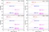 |
Fig. 6 Same as Fig. 5 but for Multiplet V19: 2s22p3d 3F°–2s22p3p 3De. |
| In the text | |
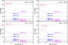 |
Fig. 7 Same as Fig. 5 but for Multiplet V39: 2s22p4f G[7/2,9/2]e–2s22p3d 3F°. |
| In the text | |
|
Fig. 8 Loci of the N ii recombination line ratios I(λ5679.56)/I(λ5666.63) and I(λ5679.56)/I(λ4041.31) for different Te’s and Ne’s. |
| In the text | |
Current usage metrics show cumulative count of Article Views (full-text article views including HTML views, PDF and ePub downloads, according to the available data) and Abstracts Views on Vision4Press platform.
Data correspond to usage on the plateform after 2015. The current usage metrics is available 48-96 hours after online publication and is updated daily on week days.
Initial download of the metrics may take a while.