| Issue |
A&A
Volume 530, June 2011
|
|
|---|---|---|
| Article Number | A17 | |
| Number of page(s) | 10 | |
| Section | Cosmology (including clusters of galaxies) | |
| DOI | https://doi.org/10.1051/0004-6361/201016040 | |
| Published online | 28 April 2011 | |
Comparison of an X-ray-selected sample of massive lensing clusters with the MareNostrum Universe ΛCDM simulation
1
INAF – Osservatorio Astronomico di Bologna, via Ranzani 1, 40127 Bologna, Italy
e-mail: This email address is being protected from spambots. You need JavaScript enabled to view it.
2
Dipartimento di Astronomia, Università di Bologna, via Ranzani 1, 40127 Bologna, Italy
3
INFN, Sezione di Bologna, Viale Berti Pichat 6/2, 40127 Bologna, Italy
4
Department of Astronomy, University of Florida, Bryant Space Science Center, Gainesville, FL, 32611, USA
5
The School of Physics and Astronomy, the Raymond and Beverly Sackler Faculty of Exact Sciences, Tel Aviv University, Tel Aviv 69978, Israel
6
Zentrum für Astronomie, Institut für Theoretische Astrophysik, Albert-Überle Str. 2, 69120 Heidelberg, Germany
7
Astrophysikalisches Institut Potsdam, An der Sternwarte 16, 14482 Potsdam, Germany
8
Grupo de Astrofísica, Universidad Autónoma de Madrid, Madrid 28049, Spain
9
Department of Theoretical Physics, University of Basque Country UPV/EHU, Leioa, Spain
10
IKERBASQUE, Basque Foundation for Science, 48011 Bilbao, Spain
Received: 2 November 2010
Accepted: 17 February 2011
Abstract
Context. A long-standing problem of strong-lensing by galaxy clusters is the observed high rate of giant gravitational arcs that are not predicted in the framework of the “standard” cosmological model. This is known as the “arc statistics problem”. Recently, several other inconsistencies between the theoretical expectations and observations have been claimed regarding the large size of the Einstein rings and the high concentrations of few clusters with strong-lensing features. All these problems consistently indicate that observed galaxy clusters may be stronger gravitational lenses than expected.
Aims. We aim at better understanding these problems by comparing the lensing properties of well defined cluster samples with those of a large set of numerically simulated objects.
Methods. We use clusters extracted from the MareNostrum Universe to build up mock catalogs of galaxy clusters selected through their X-ray flux. We use these objects to estimate the probability distributions of lensing cross sections, Einstein rings, and concentrations for a sample of 12 MACS clusters at z > 0.5 from the literature.
Results. We find that three clusters in the MACS sample have lensing cross sections and Einstein ring sizes larger than any simulated cluster in the MareNostrum Universe. We use the lensing cross sections of simulated and real clusters to estimate the number of giant arcs that should arise from lensed sources at z = 2. We find that simulated clusters produce ~50% less arcs than observed clusters do. The medians of the distributions of the Einstein ring sizes differ by ~25% between simulations and observations. We estimate that the concentrations of the individual MACS clusters inferred from the lensing analysis should be up to a factor of ~2 larger than expected from the ΛCDM model because of cluster triaxiality and orientation biases that affect the lenses with the largest cross sections. In particular, we predict that for ~20% of the clusters in the MACS sample the lensing-derived concentrations should be higher than expected by more than ~40%.
Conclusions. The arc statistics, the Einstein ring, and the concentration problems in strong lensing clusters are mitigated but not solved on the basis of our analysis. Nevertheless, owing to the lack of redshifts for most of the multiple image systems used for modeling the MACS clusters, the results of this work will need to be verified with additional data. The upcoming CLASH program will provide an ideal sample for extending our comparison.
Key words: gravitational lensing: strong / hydrodynamics / galaxies: clusters: general / dark matter
© ESO, 2011
1. Introduction
Strong lensing is a widely used method for investigating the inner structure of galaxy clusters (see Kovner 1989; Bergmann et al. 1990; Kneib et al. 2003; Broadhurst et al. 2005; Cacciato et al. 2006; Liesenborgs et al. 2009; Coe et al. 2010, for some examples). Moreover, the statistical analysis of strong lensing events in clusters was also proposed as a tool for cosmology (e.g. Bartelmann et al. 1998). The abundance of strong lensing events, such as gravitational arcs and multiple images, is expected to be higher in cosmological models where the growth of the cosmic structures is faster at earlier epochs, such as models where some dynamical dark energy starts dominating the expansion of the universe at earlier epochs (Bartelmann et al. 2003; Macciò 2005; Meneghetti et al. 2005a,b). Thus, in these models a larger number of potential lenses populates the universe up to high redshift (z > 0.5). The cluster concentrations are found in numerical simulations to reflect the density of the universe at the cluster epoch of formation. Clusters forming earlier have higher concentrations (Dolag et al. 2004) and are expected to be more efficient lenses.
In the era of precision cosmology, strong-lensing statistics cannot be as competitive as other cosmological probes for constraining cosmological parameters. These are all supporting the “concordance model” ΛCDM model, which became the standard scenario of structure formation (Komatsu et al. 2009; Riess et al. 1998, 2004; Perlmutter et al. 1999; Eisenstein et al. 2005; Percival et al. 2007). However, previous attempts of using strong-lensing statistics as a cosmological tool have produced controversial results. In particular, Bartelmann et al. (1998), studying the lensing properties of a set of numerically simulated galaxy clusters, argued that the ΛCDM cosmological model fails at reproducing the observed abundance of giant gravitational arcs by almost an order of magnitude. This inconsistency between strong-lensing and other observational data is known as the “arc statistics problem”. Its nature is still under debate. A long series of papers have tried to falsify the theoretical predictions of Bartelmann et al. (1998). Although several limits where found in their simulations, which could not properly capture several important features of both the lenses and the sources (e.g. Dalal et al. 2004; Wambsganss et al. 2004; Meneghetti et al. 2003; Torri et al. 2004; Puchwein et al. 2005; Meneghetti et al. 2007; Wambsganss et al. 2008; Mead et al. 2010), the controversy is not yet solved. Indeed, it was recently enforced by several other observations of strong lensing clusters, which seem to indicate that 1) some galaxy clusters have very extended Einstein rings (i.e. critical lines) whose abundances can hardly be reproduced by cluster models in the framework of a ΛCDM cosmology (Broadhurst & Barkana 2008; Tasitsiomi et al. 2004); and 2) several clusters, for which high-quality strong- and weak-lensing data became available, have concentrations that are far too high compared to the expectations (Broadhurst et al. 2008; Zitrin et al. 2009b). These evidences push in the same direction of the “arc statistics” problem, in the sense that they both suggest that observed galaxy clusters are strong lenses that are too effective compared to numerically simulated clusters.
Understanding the origin of these mismatches between theoretical predictions and observations is fundamental, because they may show a lack of understanding of the cluster physics, which may be not well implemented in the simulations, or, conversely, highlight some inconsistencies between the ΛCDM scenario and the properties of the universe on small scales. So far a comparison between theoretical predictions and observations has been complicated by the lack of systematic arc surveys, but also by the fact that different approaches were used to analyze simulations and observations (Meneghetti et al. 2008). In this paper, we propose a novel approach, whose principal aim is to eliminate most of the assumptions used in the previous works. It consists of analyzing observed galaxy clusters, for which detailed mass models are available through strong-, and possibly also weak-lensing observations that are fully consistent with numerical simulations. The deflection angle maps provided by the lens models are used for performing ray-tracing simulations and for lensing the same source population used in numerical simulations. We attempt a comparison between the properties of simulated clusters in the MareNostrum Universe and those of a complete sample of X-ray-luminous MACS clusters for which strong-lensing models were recently derived by Zitrin et al. (2011).
The plan of the paper is as follows. In Sects. 2 and 3 we describe the numerical and the observed cluster samples used in this study. In Sect. 4 we illustrate the analysis performed to measure the lensing cross sections and the Einstein ring sizes. In Sect. 5 we discuss the comparison between simulations and observations, describing how we construct mock cluster catalogs to simulate a MACS-like survey, and showing the statistical distributions of cross sections and Einstein rings. Finally, we use the simulated clusters for estimating the concentration bias expected for the MACS sample. Section 6 is dedicated to the discussion and the conclusions.
2. The MareNostrum Universe
Our theoretical expectations are based on the analysis of the simulated clusters contained in the MareNostrum Universe. A detailed description of the analysis performed on these objects can be found in Meneghetti et al. (2010a) and in Fedeli et al. (2010). We briefly summarize the most relevant aspects of the analysis here.
The MareNostrum Universe (Gottlöber & Yepes 2007) is a large-scale cosmological non-radiative SPH (Smooth-Particle-Hydrodynamics) simulation performed with the Gadget2 code (Springel 2005). It was performed assuming a ΛCDM cosmological background with WMAP1 normalization, namely Ωm,0 = 0.3, ΩΛ,0 = 0.7 and σ8 = 0.9 with a scale-invariant primordial power spectrum. The simulation consists of a comoving box size of 500 h-1 Mpc containing 10243 dark matter particles and 10243 gas particles. The mass of each dark matter particle equals 8.24 × 10⁹ M⊙ h-1, and that of each gas particle for which only adiabatic physics is implemented, is 1.45 × 10⁹ M⊙ h-1. The baryon density parameter is set to Ωb,0 = 0.045. The spatial force resolution is set to an equivalent Plummer gravitational softening of 15 h-1 kpc, and the SPH smoothing length was set to the 40th neighbor of each particle.
As described in Meneghetti et al. (2010a), we extracted from the cosmological box all cluster-sized halos, which were subsequently analyzed using ray-tracing techniques. Each halo was used to produce three different lens planes, obtained by projecting the cluster mass distribution along three orthogonal lines of sight. These planes of matter were used to lens a population of elliptical sources of a fixed equivalent radius of 0.5′′ placed on a source plane at redshift zs = 2. This analysis was performed on all halos found between zl = 0 and zl = 2. The strong-lensing clusters were classified into three main categories, namely 1) clusters with resolved critical lines, i.e. which can produce strong lensing features such as multiple images of the same background source; 2) clusters with a non-zero cross section for giant arcs, i.e. clusters which are potentially able to distort the images of background galaxies to form arcs with length-to-width (L/W) ratios in a way higher than 7.5; 3) what we called “super-lenses”, i.e. clusters whose lensing cross section for giant arcs is larger than 10-3 h-2 Mpc2. This definition is based on simulations including observational noises performed with the SkyLens code (Meneghetti et al. 2008, 2010b), which show that observing a cluster of galaxies with this cross section using ~3 orbits with the Hubble-Space-Telescope (HST) in the i-band, the expected number of giant arcs in the cluster field is ~1. Taking advantage of the large size of the cluster sample, we could characterize statistically the strong-lensing cluster population in the MareNostrum Universe, correlating the lensing strength to several cluster properties, such as their mass, shape, orientation, concentration, dynamical state, and X-ray emission. With ~50 000 strong-lensing clusters found in the MareNostrum Universe, this sample is the largest ever used for strong-lensing studies.
3. Strong-lensing analysis of the MACS high-redshift cluster sample
In a recent paper, Zitrin et al. (2010) showed the results of the strong-lensing analysis of a sample of 12 very luminous X-ray galaxy clusters at z > 0.5 using HST/ACS images. This is a complete sample of clusters with X-ray flux fX > 1 × 10-12 erg s-1 cm-2 in the 0.1 − 2.4 keV band, which was defined by Ebeling et al. (2007). Later, it was targeted in several follow-up studies, including deep X-ray, SZ, and HST imaging. For example, the detection of a large-scale filament has been reported for MACS J0717.5+3745 by Ebeling et al. (2004), for which many multiply-lensed images have been recently identified by Zitrin et al. (2009a), revealing this object to be the largest known lens with an Einstein radius equivalent to 55″ (for a source at z ~ 2.5). For MACS J1149.5+2223 (Zitrin & Broadhurst 2009), a background spiral galaxy at z = 1.49 (Smith et al. 2009) has been shown to be multiply-lensed into several very large images, with a total magnification factor of ~200. Another large multiply-lensed sub-mm source at a redshift of z ≃ 2.9 has been identified in MACS J0454.1-0300 (also referred to as MS 0451.6-0305; Takata et al. 2003; Borys et al. 2004; Berciano Alba et al. 2007, 2010), MACS J0025.4-1222 was found to be a “bullet cluster”-like (Bradač et al. 2008), and other MACS clusters have been recently used for an extensive arc statistics study (Horesh et al. 2010). The X-ray data available for this sample (see Ebeling et al. 2007) along with the high-resolution HST/ACS imaging and additional SZ data (e.g. LaRoque et al. 2003) make these 12 high-redshift MACS targets particularly useful for understanding the nature of the most massive clusters.
The strong-lensing modeling of this sample, published in full in Zitrin et al. (2010) and summarized briefly here, is motivated by the successful minimalistic approach of Broadhurst et al. (2005) to lens modeling, simplified further by Zitrin et al. (2009b). This simple modeling method relies on the assumption that mass traces light so that the galaxy distribution is the starting point of the mass model, and additional flexibility between the dark matter and galaxies is allowed through the implementation of external shears. Still, the method involves only six free parameters, enabling easier constraints on the mass model because the number of constraints has to be equal to or larger than the number of parameters to get a reliable fit. Two of these parameters are primarily set to reasonable values which means that only four of these parameters have to be constrained initially, which sets a very reliable starting-point using obvious systems. Recently we have further tested this assumption with Abell 1703 (Zitrin et al. 2010), where we also applied the non-parametric technique of Liesenborgs et al. (2006) for comparison. This latter technique employs an adaptive grid inversion method and does not make any prior assumptions of the mass distribution. It yields a very similar mass distribution to our parametric technique and hence confirms the assumption that mass generally traces light. In addition, it has been found independently that strong-lensing methods based on parametric modeling are accurate at the level of few percents at predicting the projected inner mass (Meneghetti et al. 2010b).
The mass distribution is therefore primarily well constrained, uncovering many multiple images which can be then iteratively incorporated into the model by using their redshift estimation and location in the image-plane (e.g., Abell 1689; Broadhurst et al. 2005, Cl0024; Zitrin et al. 2009a). In the particular case of the 12 high-z MACS clusters, in most of the clusters the multiple-images found or used in Zitrin et al. (2011) currently lack redshift information, so that the mass profiles of most of these clusters could not be well constrained but only roughly estimated by assuming crude photometric redshifts. This still allows an accurate determination of the critical curves for any given multiply-lensed source however, because the critical curves (and the mass enclosed within them) are not dependent on the mass profile and are relatively independent of the model parameters, which enables us to securely compare these properties to simulations, as done here. In addition, note that we compare the Einstein radius for sources at zs ≃ 2. Because of the lensing-distance ratios, an over-estimate of the source redshift by Δz ~ 0.5 would only increase the projected mass and the observed Einstein radius for a source at zs = 2, thus resulting only in a growth of the discrepancy between observations and the ΛCDM simulations presented here. On the other hand, underestimating a source redshift would in practice decrease the observed Einstein radius and projected mass for a source at zs = 2 by less than 10%, thus insignificantly influencing the results.
4. Analysis
4.1. Lensing cross sections
The efficiency of a galaxy cluster to produce arcs with a given property can be quantified by means of its lensing cross section. This is the area on the source plane where a source must be placed to be imaged as an arc with that property.
As explained in Meneghetti et al. (2010a) and in Meneghetti et al. (2003), the lensing cross sections are derived from the deflection angle maps, which are in turn calculated by means of ray-tracing methods (see also Meneghetti et al. 2005a,b; Fedeli et al. 2006). Bundles of light rays are traced from the observer position back to the source plane. This is populated with an adaptive grid of elliptical sources, whose spatial resolution increases toward the caustics, to artificially increase the number of highly magnified images. In the following analysis, a statistical weight, wi, which is related to the spatial resolution of the source grid at the source position, is assigned to each source. If a is the area of one pixel of the highest resolution source grid, then the area on the source plane of which the i-th source is representative is given by Ai = awi. The images are analyzed individually by measuring their lengths and widths using the method outlined in Bartelmann et al. (1998) and in Meneghetti et al. (2000).
We define the lensing cross section for giant arcs, σ, as  (1)where the sum is extended to all sources that produce at least one image with L/W > 7.5.
4.2. Einstein rings
While the lensing cross section is defined on the source plane, the Einstein ring is defined on the lens plane. Although the word “ring” is appropriate only in the case of axially symmetric lenses, several authors have used it to indicate the tangential critical line of lenses with arbitrary shapes. This is the line θt defined by the condition  (2)where λt is the inverse tangential magnification,
  . The magnification is related to the lens convergence, κ, and shear, γ, via the equation
  (3)For axially symmetric lenses the following relation holds between κ and γ:
  (4)where
  indicates the mean convergence within a circle of radius θ. Using the above formulas, the Einstein ring of an axially symmetric lens is defined as the distance θE from the lens center where
  (5)i.e. as the radius of a circle enclosing a mean convergence of 1. We remind that the convergence is related to the lens surface density Σ and to the critical surface density for lensing Σcr via the equation
  (6)Thus, the mean surface density within the Einstein ring of an axially symmetric lens is
  (7)where the Ds, Dl, and Dls denote the angular diameter distances between the observer and the source plane, between the observer and the lens plane, and between the lens and the source planes, respectively.
This is strictly applicable only to axially symmetric lenses, but this definition of Einstein ring has been exported to arbitrary lenses by several authors (see e.g. Zitrin et al. 2011; Richard et al. 2010), which define the equivalent Einstein ring size, θE,eqv, via Eq. (5). In this paper, we follow a different approach. We define a median Einstein ring size, θE,med, which is the median distance of the tangential critical points from the cluster center1:  (8)This definition better captures the significant effect of shear caused by the cluster substructures, whose effect is that of elongating the tangential critical lines along preferred directions, which pushes the critical points to distances where κ is well below unity (see also Bartelmann et al. 1995). For example, an axially symmetric lens embedded in an external shear has a larger θE,med compared to an isolated axially symmetric lens. The same argument applies to lenses whose lensing potential is elliptical rather than spherical. This is shown in Fig. 1, where we display the tangential critical lines of a lens with a Navarro-Frenk-White (NFW) density profile whose iso-potential contours have ellipticities
  equal to 0. 0.1, and 0.2. The solid, dotted, and dashed lines show the respective median Einstein rings, whose radius is derived from Eq. (8).
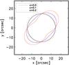 |
Fig. 1 Median Einstein rings of a lens with increasingly larger ellipticity of the lensing potential. Black, blue, and red solid lines show the tangential critical lines of lenses with ellipticity 0, 0.1, and 0.2, respectively. The corresponding median Einstein rings are given by the solid, dotted, and dashed lines of the same colors. |
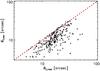 |
Fig. 2 Comparison between equivalent and median Einstein ring sizes for a sample of clusters with mass M > 5 × 10¹⁴ h-1 M⊙ at z > 0.5 extracted from the MareNostrum Universe. Each cross represents a cluster projection. The dashed red line indicates the bisector of the θE,med − θE,eqv plane. |
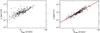 |
Fig. 3 Lensing cross section for giant arcs vs. Einstein ring size for a sample of clusters with mass M > 5 × 10¹⁴ h-1 M⊙ at z > 0.5 extracted from the MareNostrum Universe. The two panels refer to the two different definitions of the Einstein ring radius. On the left, we use the equivalent Einstein radius, while on the right we use the median Einstein radius. The red solid line in the right panel indicates the best linear fit relation between log (σ) and log (θE,med). |
In Fig. 2 we show a comparison between the two definitions of Einstein ring size when they are applied to a sample of massive clusters (M > 5 × 10¹⁴ h-1 M⊙) at redshift z > 0.5 taken from the MareNostrum Universe. Each cross represents a cluster projection in the θE,med − θE,eqv plane. Clearly, almost all points lie in the bottom-right part of the diagram, below the bisector shown by the dashed red line. Thus, θE,med ≳ θE,eqv for the vast majority of the clusters. This indicates that these systems are typically non-axially symmetric and contain many substructures that enhance their shear fields. Meneghetti et al. (2007) showed that asymmetries and substructures contribute significantly to the lensing cross section for giant arcs. Therefore, we expect that θE,med correlates much better with σ than θE,eqv does. This is shown in Fig. 3. In the left and in the right panels we plot the lensing cross section vs. the equivalent and the median Einstein ring size for the same clusters as used in Fig. 2. The figure shows that when the median Einstein radius is used, all data points lie very close to a line in the log (σ) − log (θE,med) plane, whose equation is  (9)The Pearson correlation coefficient is r = 0.94, which confirms that the correlation between the two plotted quantities is very strong.
As shown in the left panel, using the equivalent Einstein radius, the scatter is substantially larger and the correlation in much worse. The Pearson coefficient is r = 0.75 in this case. For this reason, in the following analysis we prefer to use the median, instead of the equivalent Einstein radius.
The tight correlation that exists between σ and θE,med highlights the strong connection between the arc statistics and the Einstein ring problems. If the Einstein ring sizes were too large for the ΛCDM model, we would also observe an excess of giant arcs compared to the expectations.
4.3. Analysis of the MACS sample
As we pointed out in Sect. 1, our purpose is to perform a consistent comparison between real and simulated galaxy clusters. For this reason, we use the deflection angle maps obtained for the MACS cluster reconstructions of Zitrin et al. (2011) and we use them to perform lensing simulations with the same methods as we used to analyze the clusters in the MareNostrum Universe. For each cluster, we measure the lensing cross section and the Einstein radius. Table 1 summarizes the results found for the 12 MACS clusters used in this paper. For each cluster in the sample, we also list the redshift in the second column. Note that all but two clusters have lensing cross sections for giant arcs σ > 10-3 h-2 Mpc2. On the basis of the classification proposed in Meneghetti et al. (2010a), these clusters could be classified as super-lenses.
Lensing cross sections, the median and the equivalent Einstein radii of the 12 MACS clusters used in this work.
It is very interesting to note that the θE,med − σ relation found for the MACS clusters is consistent with that measured in the MareNostrum Universe. This is shown in Fig. 4. Each diamond indicates the position of a MACS cluster in the θE,med − σ plane. The red solid line shows the best-fit relation given in Eq. (9), derived from the clusters in the MareNostrum Universe. The MACS clusters nicely follow the same relation as the one found in the simulations.
5. Comparison between simulations and observations
We now proceed to compare statistically the strong lensing properties of the MACS clusters with those of the clusters in the MareNostrum Universe.
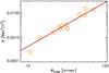 |
Fig. 4 σ − θE,med relation for the 12 MACS clusters used in this work. Each diamond indicates a cluster, while the red line is the best-fit relation found for the clusters in the MareNostrum Universe and given in Eq. (9). |
5.1. Correction of the X-ray luminosities
The MACS sample is an X-ray-flux selected sample. The selection method is discussed in Ebeling et al. (2007) and summarized later in this paper. As explained in Meneghetti et al. (2010a) we measured the X-ray emission of all clusters in the MareNostrum Universe, which, in principle, would allow us to apply the same selection function used for the MACS sample to the simulated clusters. However, the MareNostrum Universe is a non-radiative simulation, and it is well known that the X-ray properties of galaxy clusters can be reproduced only by means of a more sophisticated description of the gas physics. In particular, the X-ray luminosity of low mass clusters is known to be over-predicted in adiabatic simulations, which results in a much shallower M − LX relation than observed. A discussion about how the M − LX relation changes depending on the different gas physics can be found in Short et al. (2010). The authors of this paper show that only by including cooling and some mechanism like pre-heating or AGN feedback to heat the gas and prevent it from reaching high central densities, can the simulation match the slope of the observed M − LX relation at low redshift, as derived from the REXCESS data (Pratt et al. 2009). They also provide analytic formulas for describing the redshift evolution of the X-ray scaling relations in different kinds of simulations. In particular, the M − LX relation is parametrized as follows 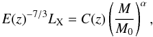 (10)where
  (11)for a spatially flat ΛCDM cosmological model, and
  (12)The parameters C0, α, and β are estimated by fitting the scaling relations of the simulated clusters. The best-fit values are reported in Tables 2 and 3 of Short et al. (2010) for different gas physics implemented in the simulations. The mass M0 is 5 × 10¹⁴ h-1 M⊙.
Using an high redshift sample of X-ray clusters from Maughan et al. (2008), the authors find that the scaling relations derived by including an AGN feedback model (FO run) evolve broadly consistently with the observational data. From Eq. (10) and the best-fit values found by Short et al. (2010) for their adiabatic (GO) and FO runs, we derive the correction we should apply to the X-ray luminosities of our simulated clusters to facilitate a comparison with the observations. This correction is estimated as 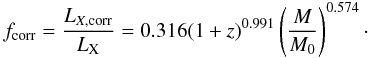 (13)
(13)
5.2. Simulating MACS-like surveys
We used the MareNostrum Universe as a reference to build up mock catalogs of MACS-like clusters. The simulated clusters are distributed on the sky within a spherical shell between z = 0.5 and z = 0.7. This volume is subdivided into seven sub-shells, which are populated with objects taken from the snapshots at z = 0.5,0.53,0.56,0.59,0.63,0.66 and 0.68 of the simulation. When necessary, we replicate the clusters in the cosmological box in a way to reproduce the expected number of halos in each shell. The number of replicates is determined by the ratio between the shell volume and the simulation volume. For the lensing analysis, each cluster is projected along three different lines of sight. Every time we replicate a cluster, we randomly choose the line of sight along which it is observed.
The sample of MACS clusters used in this work was constructed with the following selection criteria
-
the X-ray flux in the band [0.1−2.4] keV isfX > 1 × 10-12 erg s-1 cm-2;
-
the clusters are observable from Mauna Kea: |b| ≥ 20°, −40° ≤ δ ≤ 80°;
-
the redshift is z > 0.5 (the most distant cluster is at z = 0.698, as shown in Table 1).
Applying the cuts to our mock cluster catalogs, we finally define a MACS-like sample for our comparison. We repeat the procedure to generate the cluster catalogs 10 times to partially account for the cosmic variance.
5.3. Distributions of lensing cross sections
A comparison between the distributions of the lensing cross sections for giant arcs in the simulated and in the observed MACS samples is shown in Fig. 5. The histograms were normalized to the number of clusters in the observed MACS sample (12). A two-sided Kolmogorov-Smirnov test returns a probability of ~12% that the observed and simulated data are drawn from the same distribution. The most remarkable difference between the two samples is the excess of clusters with a large lensing cross section among the MACS clusters. Three clusters, namely MACS J0717.5+3745, MACS J0025.4-1222, and MACS J2129.4-0741, have lensing cross sections that exceed those of any other cluster in the MareNostrum Universe. The medians of the two distributions are σmed,MACS = 3.07 × 10⁻³ h-2 Mpc2 and σmed,MNU = 2.7 × 10⁻³ h-2 Mpc2 for the observed and for the simulated MACS samples, respectively. The lensing cross section of cluster MACS J0911.2+1746 is a factor of ~2 smaller than the smallest cross section among the simulated clusters. As shown in Fig. 4, this cluster lays below the predicted log σ − log θE,med scaling relation, i.e. the lensing cross section is small given the size of the Einstein ring.
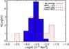 |
Fig. 5 Distributions of the strong-lensing cross sections. The blue filled histogram shows the results for the simulated MACS sample constructed with clusters taken from the MareNostrum Universe. The red shaded histogram shows the same distribution, but for the observed MACS sample. The vertical dot-dashed lines indicate the medians of the two distributions. |
The distributions can be used to estimate the differences between the expected number of giant arcs produced by the two cluster samples (when they lens sources at redshift zs = 2). The number of arcs given by  (14)where ns is the number density of sources in the background of the clusters, σi is the lensing cross section of the i-th cluster in the sample, and the sum is extended to all clusters in the sample. Using Eq. (14), we estimate that about a factor ~2 less arcs are expected from the MareNostrum clusters compared to what is expected from the MACS clusters. This is far from the order-of-magnitude difference found by Bartelmann et al. (1998) between clusters simulated in the framework of the ΛCDM cosmological model and observations and substantially reduces the size of the arc-statistics problem. This is not surprising because our simulations include the effects of mergers (Torri et al. 2004; Fedeli et al. 2006), which could not be properly taken into account by Bartelmann et al. (1998) owing to the limited number of clusters in their sample and to the coarse time resolution in their simulations. Analyzing the MareNostrum Universe, we showed in Fedeli et al. (2010) that unrelaxed clusters contribute to ~70% of the optical depth for clusters at z > 0.5.
5.4. Distributions of Einstein ring sizes
In Fig. 6 we compare the distributions of the Einstein ring sizes for the simulated and the observed MACS samples. As found for the lensing cross sections, the distribution derived for the observed cluster sample is also characterized by an excess of clusters toward the high values of θE. The same clusters that have larger cross sections compared to any simulated cluster also have Einstein radii exceeding the maximum value found in the simulations. The Kolmogorov-Smirnov test returns a probability of ~30% that the two datasets are drawn from the same statistical distribution. The Einstein ring medians of the observed and of the simulated samples differ by ~25%, while Zitrin et al. (2011) report a difference of ~40% between the observed and the theoretical distributions of Einstein radii. However, their theoretical estimates are based on analytic models of galaxy clusters that are described by means of axially symmetric lenses with NFW density profiles. Meneghetti et al. (2003) showed that these simple lens models underestimate the lensing cross sections for giant arcs of numerically simulated clusters, mainly because they miss several important features like asymmetries and substructures, which significantly enhance the lensing efficiency of galaxy clusters (see also Meneghetti et al. 2007). Given the strong correlation between lensing cross section and Einstein radius, shown in Fig. 3, it is not surprising that our numerically simulated galaxy clusters have larger Einstein radii. Thus, as with the arc statistics problem, also the Einstein ring problem is alleviated on the basis of our results, although three clusters still do not have a counterpart in our ΛCDM simulation.
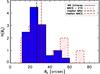 |
Fig. 6 Distributions of the Einstein ring sizes. The blue filled histogram shows the results for the simulated MACS sample constructed with clusters taken from the MareNostrum Universe. The red shaded histogram shows the same distribution, but for the observed MACS sample. The vertical dot-dashed lines indicate the medians of the two distributions. |
5.5. Expected concentration bias
Meneghetti et al. (2010a) showed that, owing to the cluster triaxiality and to the orientation bias that affects the strong lensing cluster population, we should expect to measure substantially higher concentrations than expected in clusters that show many strong lensing features (see also Oguri et al. 2005, 2009). Indeed, the amplitude of this bias is a growing function of the lensing cross section. It is rewarding (and easy) to estimate the bias that is expected to affect a MACS-like sample of clusters. For each of the clusters in the simulated sample we measure the concentration inferred from both the projected and the three-dimensional mass distributions, c2D and c3D. These are measured by the surface mass density and the three-dimensional mass density with the NFW models. The concentration bias is quantified by means of the ratio between the two-dimensional and the three-dimensional concentrations.
The distribution of c2D/c3D derived from the simulated MACS sample is shown in Fig. 7. As expected, a median bias on the order of ~11% is found. However, the distribution is skewed toward the high values. On the basis of our simulations we expect that the concentration may be biased by up to 100% for some of the clusters. The dashed line shows the cumulative probability distribution. For about ~20% of the clusters in the simulated sample we measure a two-dimensional concentration that is >40% higher than the three-dimensional concentration.
In Fig. 8 we show how the concentration bias depends on the lensing cross section. While the bias is very small, on the order of a few percent for clusters with σ < 10-3 h-2 Mpc2, it becomes increasingly higher for the clusters with larger cross sections. This is a very important result for interpreting the high concentrations recently measured in clusters like A1689 or CL0024 (Broadhurst et al. 2008; Zitrin et al. 2009b).
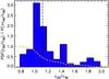 |
Fig. 7 Probability density function of the ratios between two-dimensional and three-dimensional concentrations for clusters with the same properties as those in the MACS sample. The vertical dot-dashed line indicates the median of the distribution. The dashed line shows the cumulative distribution. |
 |
Fig. 8 Concentration bias vs. the strong-lensing cross section. Each square represents a simulated cluster from a mock MACS catalog. The solid line is the median relation, while the error-bars indicate the inter-quartile ranges in each bin. |
6. Discussion and conclusions
We used a large set of numerically simulated clusters for which the X-ray and the lensing properties were previously investigated, and compared their Einstein ring sizes and strong-lensing cross sections to those of clusters in an X-ray selected sample at redshift z > 0.5 (MACS). We also used the numerical simulations to estimate the expected bias in the lensing-inferred concentrations of the same MACS sample. Our aim was to investigate whether some previously claimed discrepancies between the strong-lensing properties of real and analytically modeled clusters in the framework of ΛCDM cosmology were confirmed by adopting more sophisticated and realistic cluster mass distributions. These discrepancies between theory and observations regard 1) the large observed number of gravitational arcs behind the cores of galaxy clusters; 2) the large size of the Einstein rings reconstructed through lensing-based observations; and 3) the large mass concentrations determined by fitting the two-dimensional mass distribution of strong lensing clusters. Our main results can be summarized as follows:
-
the comparison between the numerical and the observationalcluster sample shows that some real clusters have lensing crosssections and Einstein rings that are too large compared to theexpectations in a ΛCDM cosmological model. However, the discrepancy between observations and simulations is now significantly reduced compared to previous studies based on analytical estimates. Using N-body and hydrodynamical simulations allows one to better capture several important properties of the strong-lensing clusters, such as their triaxiality, asymmetries, concentration scatter, and dynamical activity, all of which were proven to boost the lensing efficiency;
-
using numerically simulated clusters we can predict the lensing concentration bias expected for the MACS sample. This estimate is based on the assumption that the numerical models are representative of the real cluster population. As shown by our results on the lensing cross sections and on the size of the Einstein rings, this may not be the case. Measuring a larger-than-expected concentration bias in real clusters may be a further indication that some substantial difference exists between the inner structure of observed and simulated clusters.
We believe that these results are important because they suggest that our simplified models of the physical processes that affect the matter distribution in the cores of galaxy clusters must be improved. First of all this improvement concerns the description of gas-dynamical processes in clusters. On the other hand, our results may also indicate that some fundamental assumption in the ΛCDM model is incorrect and leads to wrong predictions of the matter distribution on scales probed by galaxy clusters. In this case, alternative cosmologies that involve dynamical dark-energy, modified gravity, or primordial non-Gaussianity may better explain the differences between the strong lensing properties of simulated and observed galaxy clusters.
However, a few aspects of our work deserve some further discussion and deeper investigation. The simulations used in this study are performed in the framework of a WMAP-1 normalized cosmology. The value of σ8 used in this study is higher than measured in the WMAP-7 data release. If the WMAP-7 normalization were adopted, the differences between simulations and observations would be significantly amplified. Fedeli et al. (2008) show that if one decreases σ8 from 0.9 to 0.8, the average lensing optical depth drops by at least a factor of three. The cluster efficiency for strong lensing would be strongly dimmed at z > 0.5, as a result of the delayed structure formation caused by a lower normalization of the CDM power-spectrum. Duffy et al. (2008) showed that the typical concentration of clusters simulated in a WMAP-5 cosmological framework is lower than in the case of a WMAP-1 normalized cosmology (~16% lower at the cluster mass scale).
Our simulations suffer of two important limitations. The first is certainly given by the size of the cosmological box. Owing to the relatively small box size, we may be underpredicting the number of very high-mass clusters in the sample. Moreover, we may be missing some systems that are particularly dynamically active. Consequently, our numerical sample may miss some of the most powerful lenses. We will investigate this problem by using a sample of massive clusters extracted from a larger cosmological box. The second limitation is due to the simple description of the gas physics in the simulation, where no radiative and feedback processes are considered. On the basis of the recent results of Mead et al. (2010), we are confident that this does not significantly affect the lensing properties of the clusters. It has been shown that the energy feedback from AGNs and supernovae counteract and compensate the effects of cooling on the strong lensing cross sections. However, as we explained earlier, the X-ray scaling relations are strongly affected by these physical processes. We introduced a correction to the X-ray fluxes based on the comparison between simulations and observations for accounting for this poor description of the gas physics. Without more sophisticated cluster models, this was the only viable approach, which is based on several approximation however. Gas physics also influence the cluster concentrations, as shown by Duffy et al. (2010), who found that the actions of the supernovae and AGN are to remove so much gas (in order to match observed stellar fractions in these systems) that the concentration is reduced by up to 20%.
As mentioned in Sect. 3, most of the multiple image systems detected behind the MACS clusters do not have spectroscopically confirmed redshifts. This lack of information makes these cluster mass reconstructions uncertain, although we believe that our conclusions would not be dramatically affected (see the discussion in the Appendix A). This situation will be soon improved thanks to the upcoming Hubble Multi-Cycle-Treasury-Program CLASH2, which will dedicate 524 new HST orbits to observe 25 galaxy clusters in 16 different bands, spanning the near-UV to near-IR (P.I. Postman). These observations, combined with already existing data for some of the targets, are expected to deliver ~40 new multiple image systems per cluster with a photometric redshift determined with an accuracy Δz ~ 0.02(1 + z). Half of the clusters in the MACS sample used in this paper are also in the CLASH target list. As shown by Meneghetti et al. (2010b), these observations will allow us to constrain the Einstein ring sizes and the projected mass distributions in the inner regions of clusters with accuracies at the percent level. We look forward to improving our comparison between observations and simulations using this new dataset as well as improved cosmological simulations.
While our paper was in the process of being refereed, Horesh et al. (2011) posted a paper were a comparison between the lensed ac statistics by simulated halos taken from the Millennium simulation (Springel et al. 2005) and by a sample of X-ray selected clusters is shown. Their results for z > 0.5 agree with ours, being the simulated arc production efficiency lower by a factor of 3 than observed in the MACS cluster sample. Instead, at lower redshift (z ~ 0.4), they find a very good agreement between the observed and the simulated arc statistics, in terms of the mean number of arcs per cluster, the distribution of number of arcs per clusters, and the angular separation distribution. At even lower redshift, (z ~ 0.2) they again find an excess of arcs in the observations compared to simulations. Clearly, this emphasises that we need much larger samples before we arrive at a firm conclusion.
When dealing with mass distributions characterized by asymmetries and substructures, the cluster center may not be easily defined. In this work, the cluster center is determined by smoothing the projected cluster mass distribution with a Gaussian kernel with a FWHM of 30 kpc. This is meant to erase the local peaks that are related to the presence of galaxy-scale halos. The center of the cluster is then defined as the location of the maximum of the smoothed projected mass distribution. This is only one of the possible choices for the cluster center. Of course, the same definition holds for simulated and real clusters.
Acknowledgments
M.M. thanks Elena Rasia and Pasquale Mazzotta for their useful comments on this work. We are grateful to M. Limousin for carefully revising our paper and for providing us the models of some some of the MACS clusters. We acknowledge financial contributions from contracts ASI-INAF I/023/05/0, ASI-INAF I/088/06/0, ASI-INAF I/009/10/0, and PRIN INAF 2009. The MareNostrum Universe simulation was made at the BSC-CNS (Spain) and analyzed at NIC Jülich (Germany). S.G. acknowledges the support of the European Science Foundation through the ASTROSIM Exchange Visits Program. G.Y. acknowledges support of MICINN (Spain) through research grants FPA2009-08958 and AYA2009-13875-C03-02.
References
- Bartelmann, M., Steinmetz, M., & Weiss, A. 1995, A&A, 297, 1 [NASA ADS] [Google Scholar]
- Bartelmann, M., Huss, A., Colberg, J., Jenkins, A., & Pearce, F. 1998, A&A, 330, 1 [NASA ADS] [Google Scholar]
- Bartelmann, M., Meneghetti, M., Perrotta, F., Baccigalupi, C., & Moscardini, L. 2003, A&A, 409, 449 [NASA ADS] [CrossRef] [EDP Sciences] [Google Scholar]
- Berciano Alba, A., Garrett, M. A., Koopmans, L. V. E., & Wucknitz, O. 2007, A&A, 462, 903 [NASA ADS] [CrossRef] [EDP Sciences] [Google Scholar]
- Berciano Alba, A., Koopmans, L. V. E., Garrett, M. A., Wucknitz, O., & Limousin, M. 2010, A&A, 509, A54 [NASA ADS] [CrossRef] [EDP Sciences] [Google Scholar]
- Bergmann, A. G., Petrosian, V., & Lynds, R. 1990, ApJ, 350, 23 [NASA ADS] [CrossRef] [Google Scholar]
- Borys, C., Chapman, S., Donahue, M., et al. 2004, MNRAS, 352, 759 [NASA ADS] [CrossRef] [Google Scholar]
- Bradač, M., Allen, S. W., Treu, T., et al. 2008, ApJ, 687, 959 [NASA ADS] [CrossRef] [Google Scholar]
- Broadhurst, T. J., & Barkana, R. 2008, MNRAS, 390, 1647 [NASA ADS] [Google Scholar]
- Broadhurst, T., Benítez, N., Coe, D., et al. 2005, ApJ, 621, 53 [NASA ADS] [CrossRef] [Google Scholar]
- Broadhurst, T., Umetsu, K., Medezinski, E., Oguri, M., & Rephaeli, Y. 2008, ApJ, 685, L9 [NASA ADS] [CrossRef] [Google Scholar]
- Cacciato, M., Bartelmann, M., Meneghetti, M., & Moscardini, L. 2006, A&A, 458, 349 [NASA ADS] [CrossRef] [EDP Sciences] [Google Scholar]
- Coe, D., Benitez, N., Broadhurst, T., Moustakas, L., & Ford, H. 2010, ApJ, 723, 1678 [NASA ADS] [CrossRef] [Google Scholar]
- Dalal, N., Holder, G., & Hennawi, J. F. 2004, ApJ, 609, 50 [NASA ADS] [CrossRef] [Google Scholar]
- Dolag, K., Bartelmann, M., Perrotta, F., et al. 2004, A&A, 416, 853 [NASA ADS] [CrossRef] [EDP Sciences] [Google Scholar]
- Duffy, A. R., Schaye, J., Kay, S. T., & Dalla Vecchia, C. 2008, MNRAS, 390, L64 [NASA ADS] [CrossRef] [Google Scholar]
- Duffy, A. R., Schaye, J., Kay, S. T., et al. 2010, MNRAS, 405, 2161 [NASA ADS] [Google Scholar]
- Ebeling, H., Barrett, E., & Donovan, D. 2004, ApJ, 609, L49 [Google Scholar]
- Ebeling, H., Barrett, E., Donovan, D., et al. 2007, ApJ, 661, L33 [NASA ADS] [CrossRef] [Google Scholar]
- Eisenstein, D. J., Zehavi, I., Hogg, D. W., et al. 2005, ApJ, 633, 560 [NASA ADS] [CrossRef] [Google Scholar]
- Fedeli, C., Meneghetti, M., Bartelmann, M., Dolag, K., & Moscardini, L. 2006, A&A, 447, 419 [NASA ADS] [CrossRef] [EDP Sciences] [Google Scholar]
- Fedeli, C., Bartelmann, M., Meneghetti, M., & Moscardini, L. 2008, A&A, 486, 35 [NASA ADS] [CrossRef] [EDP Sciences] [Google Scholar]
- Fedeli, C., Meneghetti, M., Gottloeber, S., & Yepes, G. 2010, A&A, 519, A91 [NASA ADS] [CrossRef] [EDP Sciences] [Google Scholar]
- Gottlöber, S., & Yepes, G. 2007, ApJ, 664, 117 [NASA ADS] [CrossRef] [Google Scholar]
- Horesh, A., Maoz, D., Ebeling, H., Seidel, G., & Bartelmann, M. 2010, MNRAS, 406, 1318 [NASA ADS] [Google Scholar]
- Horesh, A., Maoz, D., Hilbert, S., & Bartelmann, M. 2011, MNRAS, submitted [arXiv:1101.4653] [Google Scholar]
- Kneib, J., Hudelot, P., Ellis, R. S., et al. 2003, ApJ, 598, 804 [NASA ADS] [CrossRef] [Google Scholar]
- Komatsu, E., Dunkley, J., Nolta, M. R., et al. 2009, ApJS, 180, 330 [NASA ADS] [CrossRef] [Google Scholar]
- Kovner, I. 1989, ApJ, 337, 621 [NASA ADS] [CrossRef] [Google Scholar]
- LaRoque, S. J., Joy, M., Carlstrom, J. E., et al. 2003, ApJ, 583, 559 [NASA ADS] [CrossRef] [Google Scholar]
- Liesenborgs, J., De Rijcke, S., & Dejonghe, H. 2006, MNRAS, 367, 1209 [NASA ADS] [CrossRef] [Google Scholar]
- Liesenborgs, J., de Rijcke, S., Dejonghe, H., & Bekaert, P. 2009, MNRAS, 397, 341 [NASA ADS] [CrossRef] [Google Scholar]
- Limousin, M., Ebeling, H., Ma, C., et al. 2010, MNRAS, 405, 777 [NASA ADS] [Google Scholar]
- Macciò, A. V. 2005, MNRAS, 361, 1250 [NASA ADS] [CrossRef] [Google Scholar]
- Maughan, B. J., Jones, C., Forman, W., & Van Speybroeck, L. 2008, ApJS, 174, 117 [NASA ADS] [CrossRef] [Google Scholar]
- Mead, J. M. G., King, L. J., Sijacki, D., et al. 2010, MNRAS, 406, 434 [NASA ADS] [CrossRef] [Google Scholar]
- Meneghetti, M., Bolzonella, M., Bartelmann, M., Moscardini, L., & Tormen, G. 2000, MNRAS, 314, 338 [NASA ADS] [CrossRef] [Google Scholar]
- Meneghetti, M., Bartelmann, M., & Moscardini, L. 2003, MNRAS, 340, 105 [NASA ADS] [CrossRef] [Google Scholar]
- Meneghetti, M., Bartelmann, M., Dolag, K., et al. 2005a, A&A, 442, 413 [NASA ADS] [CrossRef] [EDP Sciences] [Google Scholar]
- Meneghetti, M., Jain, B., Bartelmann, M., & Dolag, K. 2005b, MNRAS, 362, 1301 [NASA ADS] [CrossRef] [Google Scholar]
- Meneghetti, M., Argazzi, R., Pace, F., et al. 2007, A&A, 461, 25 [NASA ADS] [CrossRef] [EDP Sciences] [Google Scholar]
- Meneghetti, M., Melchior, P., Grazian, A., et al. 2008, A&A, 482, 403 [NASA ADS] [CrossRef] [EDP Sciences] [Google Scholar]
- Meneghetti, M., Fedeli, C., Pace, F., Gottloeber, S., & Yepes, G. 2010a, A&A, 519, A90 [NASA ADS] [CrossRef] [EDP Sciences] [Google Scholar]
- Meneghetti, M., Rasia, E., Merten, J., et al. 2010b, A&A, 514, A93 [NASA ADS] [CrossRef] [EDP Sciences] [Google Scholar]
- Oguri, M., Takada, M., Umetsu, K., & Broadhurst, T. 2005, ApJ, 632, 841 [NASA ADS] [CrossRef] [Google Scholar]
- Oguri, M., Hennawi, J. F., Gladders, M. D., et al. 2009, ApJ, 699, 1038 [NASA ADS] [CrossRef] [Google Scholar]
- Percival, W. J., Cole, S., Eisenstein, D. J., et al. 2007, MNRAS, 381, 1053 [NASA ADS] [CrossRef] [MathSciNet] [Google Scholar]
- Perlmutter, S., Aldering, G., Goldhaber, G., et al. 1999, ApJ, 517, 565 [NASA ADS] [CrossRef] [Google Scholar]
- Pratt, G. W., Croston, J. H., Arnaud, M., & Böhringer, H. 2009, A&A, 498, 361 [NASA ADS] [CrossRef] [EDP Sciences] [Google Scholar]
- Puchwein, E., Bartelmann, M., Dolag, K., & Meneghetti, M. 2005, A&A, 442, 405 [Google Scholar]
- Richard, J., Smith, G. P., Kneib, J., et al. 2010, MNRAS, 404, 325 [NASA ADS] [Google Scholar]
- Riess, A. G., Filippenko, A. V., Challis, P., et al. 1998, AJ, 116, 1009 [NASA ADS] [CrossRef] [Google Scholar]
- Riess, A., Strolger, L.-G., Tonry, J., et al. 2004, ApJ, 607, 665 [NASA ADS] [CrossRef] [Google Scholar]
- Short, C. J., Thomas, P. A., Young, O. E., et al. 2010, MNRAS, 408, 2213 [NASA ADS] [CrossRef] [Google Scholar]
- Smith, G. P., Ebeling, H., Limousin, M., et al. 2009, ApJ, 707, L163 [NASA ADS] [CrossRef] [Google Scholar]
- Springel, V. 2005, MNRAS, 364, 1105 [NASA ADS] [CrossRef] [Google Scholar]
- Springel, V., White, S. D. M., Jenkins, A., et al. 2005, Nature, 435, 629 [NASA ADS] [CrossRef] [PubMed] [Google Scholar]
- Takata, T., Kashikawa, N., Nakanishi, K., et al. 2003, PASJ, 55, 789 [NASA ADS] [Google Scholar]
- Tasitsiomi, A., Kravtsov, A. V., Gottlöber, S., & Klypin, A. A. 2004, ApJ, 607, 125 [Google Scholar]
- Torri, E., Meneghetti, M., Bartelmann, M., et al. 2004, MNRAS, 349, 476 [NASA ADS] [CrossRef] [Google Scholar]
- Wambsganss, J., Bode, P., & Ostriker, J. 2004, ApJ, 606, L93 [NASA ADS] [CrossRef] [Google Scholar]
- Wambsganss, J., Ostriker, J. P., & Bode, P. 2008, ApJ, 676, 753 [NASA ADS] [CrossRef] [Google Scholar]
- Zitrin, A., & Broadhurst, T. 2009, ApJ, 703, L132 [NASA ADS] [CrossRef] [Google Scholar]
- Zitrin, A., Broadhurst, T., Rephaeli, Y., & Sadeh, S. 2009a, ApJ, 707, L102 [NASA ADS] [CrossRef] [Google Scholar]
- Zitrin, A., Broadhurst, T., Umetsu, K., et al. 2009b, MNRAS, 396, 1985 [NASA ADS] [CrossRef] [Google Scholar]
- Zitrin, A., Broadhurst, T., Umetsu, K., et al. 2010, MNRAS, 408, 1916 [NASA ADS] [CrossRef] [Google Scholar]
- Zitrin, A., Broadhurst, T., Barkana, R., Rephaeli, Y., & Benitez, N. 2011, MNRAS, 410, 1939 [NASA ADS] [Google Scholar]
Appendix A: How stable are the MACS lens models?
As we pointed out earlier, the major source of uncertainty in the mass models of the MACS clusters used in this study is the lack of spectroscopic redshifts available for most of the multiple image systems. Indeed, for several of these systems the redshifts are estimated photometrically. Other groups who performed a strong-lensing analysis on some of the clusters used in this study did not agree on the identification of several strong-lensing systems. To appraise how stable the models are with respect to the assumptions made, we here compare some of the models of Zitrin et al. (2011) (Z models in the following) with alternative models kindly provided by Marceu Limousin. It is important to note that 1) these models are obtained with a completely different mass reconstruction code, the public software lenstool3, which follows a completely different approach compared to Zitrin et al. (2011); and 2) in some cases the associations and the number of multiple image systems differ significantly.
The lenstool models (L models hereafter) were provided for four of the MACS clusters under investigation. These are the clusters MACS J0717.5+3745 (Limousin et al., in prep.), MACS J1149.5+2223 (see details in Smith et al. 2009), MACS J0454.1-0300 (Berciano Alba et al. 2007, 2010), and MACS J1423.8+2404 (Limousin et al. 2010). We use these models fully consistently with the analysis made on the Z reconstructions, to derive measurements of the Einstein rings and of the lensing cross sections.
The L model of MACS J0717 is based on a set of 15 multiple image systems, the vast majority of which agree with the systems identified and used by Zitrin et al. (2011). Recently Limousin and collaborators gathered spectroscopic redshifts for two of these systems, which have been used to calibrate their model. The resulting reconstruction has an Einstein ring θmed = 61′′ and a lensing cross section σ = 1.24 × 10² h-2 Mpc-2. These values are only ~15% lower than those of the corresponding Z model.
In MACS J1149, the most spectacular lensed system is a spiral galaxy whose total magnification is estimated to be ~200. According to Zitrin & Broadhurst (2009) and Zitrin et al. (2011) (Z model), this galaxy is lensed into five images, while Smith et al. (2009) refer to the fifth image as part of the fourth image. This of course is a matter of interpretation. The calibration of the Z model is based on the assumption that the redshift of the above mentioned spiral galaxy is ~1.5, which was then spectroscopically confirmed by Smith et al. (2009). Additionally, the Z lens model itself has allowed us to identify six additional multiple-image candidate systems, which are not used in the construction of the L model nor are plausible in this model. The mass reconstructions derived from the constraints used by the two groups differ correspondingly. In particular, the Z model has a shallower projected density profile than the L model. Despite this, the two models result to be almost identical in terms of both Einstein ring and lensing cross section, with differences on the order of only a few percent.
Using the L model of MACS J1423 we find an Einstein ring and a cross section that are respectively ~30% and ~25% smaller than those derived from the Z model. Strangely, for this cluster spectroscopic redshifts exist for two sets of multiple images which are used to build both the L and the Z models, thus this mismatch between the models was quite unexpected. However, by visually inspecting the critical lines of the two reconstructions, we notice that the Z model predicts a northward extension of the tangential critical line, which surrounds a bright elliptical galaxy (see Fig. 19 of Zitrin et al. 2011). This extension is not present in the L model and contributes to increasing both θE and σ. It may be an artifact or not, depending on the still unknown weight of this galaxy, because there are no lensing constraints in that region of the lens plane that probe this portion of the critical curve.
MACS J0454 shows the largest discrepancy between L and Z models. In this case, the Einstein ring size and the lensing cross section derived from the L model far exceed those derived from the Z model (a factor of two and a factor of five, respectively). We do not fully understand the origin of this mismatch. The Z model is built with the same lensing constraints as the L model, including also the spectroscopic redshift of one system at zs = 2.9. The Z model is also validated by an additional two systems of multiply-lensed images, which were identified thanks to the model itself. Therefore, we are confident that the Z model used in the analysis is better constrained than the L model.
To summarize, we find a good agreement between Z and L models in three out of four of the MACS clusters used in this comparison, while for the fourth cluster, we think that the Z model is better constrained, which supports our results. Therefore, we are confident that out results are robust. In the σ − θE plane, even the L models do not significantly depart from the relation fitted to the simulations. This is shown in Fig. A.1, which shows with sticks and diamonds the new locations of the four MACS clusters when they are modeled with lenstool, and their shift with respect to the corresponding Z models. These are overlaid to Fig. 4 for comparison.
 |
Fig. A.1 Shift of the some of the MACS clusters in the σ − θE, when alternative models obtained with lenstool are used to derive the Einstein rings and the lensing cross sections. |
All Tables
Lensing cross sections, the median and the equivalent Einstein radii of the 12 MACS clusters used in this work.
All Figures
|
Fig. 1 Median Einstein rings of a lens with increasingly larger ellipticity of the lensing potential. Black, blue, and red solid lines show the tangential critical lines of lenses with ellipticity 0, 0.1, and 0.2, respectively. The corresponding median Einstein rings are given by the solid, dotted, and dashed lines of the same colors. |
| In the text | |
|
Fig. 2 Comparison between equivalent and median Einstein ring sizes for a sample of clusters with mass M > 5 × 10¹⁴ h-1 M⊙ at z > 0.5 extracted from the MareNostrum Universe. Each cross represents a cluster projection. The dashed red line indicates the bisector of the θE,med − θE,eqv plane. |
| In the text | |
|
Fig. 3 Lensing cross section for giant arcs vs. Einstein ring size for a sample of clusters with mass M > 5 × 10¹⁴ h-1 M⊙ at z > 0.5 extracted from the MareNostrum Universe. The two panels refer to the two different definitions of the Einstein ring radius. On the left, we use the equivalent Einstein radius, while on the right we use the median Einstein radius. The red solid line in the right panel indicates the best linear fit relation between log (σ) and log (θE,med). |
| In the text | |
|
Fig. 4 σ − θE,med relation for the 12 MACS clusters used in this work. Each diamond indicates a cluster, while the red line is the best-fit relation found for the clusters in the MareNostrum Universe and given in Eq. (9). |
| In the text | |
|
Fig. 5 Distributions of the strong-lensing cross sections. The blue filled histogram shows the results for the simulated MACS sample constructed with clusters taken from the MareNostrum Universe. The red shaded histogram shows the same distribution, but for the observed MACS sample. The vertical dot-dashed lines indicate the medians of the two distributions. |
| In the text | |
|
Fig. 6 Distributions of the Einstein ring sizes. The blue filled histogram shows the results for the simulated MACS sample constructed with clusters taken from the MareNostrum Universe. The red shaded histogram shows the same distribution, but for the observed MACS sample. The vertical dot-dashed lines indicate the medians of the two distributions. |
| In the text | |
|
Fig. 7 Probability density function of the ratios between two-dimensional and three-dimensional concentrations for clusters with the same properties as those in the MACS sample. The vertical dot-dashed line indicates the median of the distribution. The dashed line shows the cumulative distribution. |
| In the text | |
|
Fig. 8 Concentration bias vs. the strong-lensing cross section. Each square represents a simulated cluster from a mock MACS catalog. The solid line is the median relation, while the error-bars indicate the inter-quartile ranges in each bin. |
| In the text | |
|
Fig. A.1 Shift of the some of the MACS clusters in the σ − θE, when alternative models obtained with lenstool are used to derive the Einstein rings and the lensing cross sections. |
| In the text | |
Current usage metrics show cumulative count of Article Views (full-text article views including HTML views, PDF and ePub downloads, according to the available data) and Abstracts Views on Vision4Press platform.
Data correspond to usage on the plateform after 2015. The current usage metrics is available 48-96 hours after online publication and is updated daily on week days.
Initial download of the metrics may take a while.