| Issue |
A&A
Volume 529, May 2011
|
|
|---|---|---|
| Article Number | A162 | |
| Number of page(s) | 10 | |
| Section | Extragalactic astronomy | |
| DOI | https://doi.org/10.1051/0004-6361/201116541 | |
| Published online | 25 April 2011 | |
Polarimetry of optically selected BL Lacertae candidates from the SDSS⋆,⋆⋆,⋆⋆⋆,†
1
ZAH, Landessternwarte Heidelberg, Königstuhl,
69117
Heidelberg,
Germany
e-mail: This email address is being protected from spambots. You need JavaScript enabled to view it.
2
Finnish Centre for Astronomy with ESO (FINCA), University of
Turku, Väisäläntie
20, 21500
Piikkiö,
Finland
Received: 18 January 2011
Accepted: 18 February 2011
Abstract
We present and discuss polarimetric observations of 182 targets drawn from an optically selected sample of 240 probable BL Lac candidates out of the SDSS compiled by Collinge et al. (2005, AJ, 129, 2542). In contrast to most other BL Lac candidate samples extracted from the SDSS, its radio- and/or X-ray properties have not been taken into account for its derivation. Thus, because its selection is based on optical properties alone, it may be less prone to selection effects inherent in other samples derived at different frequencies, so it offers a unique opportunity to extract the first unbiased BL Lac luminosity function that is suitably large in size.
We found 124 out of 182 targets (68%) to be polarized, 95 of the polarized targets (77%) to be highly polarized (>4%). The low-frequency peaked BL Lac candidates in the sample are on average only slightly more polarized than the high-frequency peaked ones. Compared to earlier studies, we found a high duty cycle in high polarization ( to be >4% polarized) in high-frequency peaked BL Lac candidates. This may come from our polarization analysis, which minimizes the contamination by host galaxy light.
No evidence of radio-quiet BL Lac objects in the sample was found.
Our observations show that the probable sample of BL Lac candidates of Collinge et al. (2005) indeed contains a large number of bona fide BL Lac objects. High S/N spectroscopy and deep X-ray observations are required to construct the first luminosity function of optically selected BL Lac objects and to test more stringently for any radio-quiet BL Lac objects in the sample.
Key words: polarization / techniques: polarimetric / BL Lacertae objects: general / galaxies: active
Based on observations collected with the NTT on La Silla (Chile) operated by the European Southern Observatory in the course of the observing proposal 082.B-0133.
Based on observations collected at the Centro Astronómico Hispano Alemán (CAHA), operated jointly by the Max-Planck-Institut für Astronomie and the Instituto de Astrofisica de Andalucia (CSIC).
Based on observations made with the Nordic Optical Telescope, operated on the island of La Palma jointly by Denmark, Finland, Iceland, Norway, and Sweden, in the Spanish Observatorio del Roque de los Muchachos of the Instituto de Astrofisica de Canarias.
Table 1 is only available in electronic form at the CDS via anonymous ftp to cdsarc.u-strasbg.fr (130.79.128.5) or via http://cdsarc.u-strasbg.fr/viz-bin/qcat?J/A+A/529/A162
© ESO, 2011
1. Introduction
BL Lac objects are characterized by large variability from radio to TeV frequencies, nearly featureless optical spectra, high and variable polarization, and in many cases superluminal motion. They reside in the nuclei of giant elliptical galaxies, where according to the current paradigm, a supermassive black hole is accreting material from its surroundings and collimating two relativistic jets in opposite directions. According to the so-called “Unified Scheme” (Urry & Padovani 1995), BL Lac objects are FR I radio galaxies with one of the jets nearly pointing towards us. Relativistic effects can boost the jet emission to a level where it almost completely outshines the host galaxy.
Due to their extreme properties it is not surprising that BL Lacs form <1% of the entire AGN population known today. More than 100 000 confirmed QSO’s (Schneider et al. 2010) and more than 106 QSO candidates (Richards et al. 2009) have been published, but the number of BL Lac (candidates) hardly exceeds 1000 (Véron-Cetty & Véron 2010).
BL Lac objects are classically detected in radio- or X-ray surveys and have traditionally been divided into two groups according to the location of the peak of their synchrotron emission: the low-energy-peaked BL Lacs (LBL) and high-energy-peaked BL Lacs (HBL). Until now, the resulting samples based on single surveys alone only contain a few dozen objects, irrespective of whether they have been compiled from radio (e.g. the 1Jy sample by Stickel et al. 1991) or from X-ray observations (e.g. the Einstein Slew Survey sample by Perlman et al. 1996). Samples compiled from a combination of both, e.g., the ROSAT All-Sky Survey-Green Bank sample by Laurent-Muehleisen et al. (1999, RGB) and the Sedentary Survey by Giommi et al. (2005) contain a much larger number of objects (100−200). Most important is that they contain BL Lac objects midway between LBL and HBL. Regardless of the selection criteria, all samples suffer from a relatively high number of up to 50% of sources with unknown or highly uncertain redshift and are subject to various biases by their selection criteria. BL Lacs detected in radio surveys are typically more core-dominated than those detected in X-rays, and the surveys in different wavelength regimes have different depths.
Claims have been made that HBL and LBL may evolve differently (Stickel et al. 1991; Morris et al. 1991), but these claims are subject to low number statistics and to the biases mentioned above, which cannot be easily corrected for. Likewise, the general trend in the cosmic evolution of BL Lacs is not constrained, with claims of negative, positive, or no evolution (see e.g. Beckmann et al. 2003; Padovani et al. 2007). As a consequence, attempts to construct, say, a luminosity function for BL Lacs and/or their hosts were limited by small numbers (Padovani et al. 2007). The former is especially important since it allows a test of the Unified Scheme and can constrain models for jet opening angles as a function of luminosity by comparing it with the luminosity functions of other radio-loud AGN.
A viable alternative would be to construct a suitable optically selected sample of BL Lac objects. Since the optical region lies between the HBL and LBL peak frequencies, optically selected samples are representative of the whole BL Lac population and may be subject to biases that are easier to control. However, besides the obvious advantage of optically selected BL Lac samples over the ones selected from radio and/or X-ray surveys, only a few attempts have been made to extract an optically selected sample of BL Lacs. Exactly because BL Lac objects share optical properties with other sources (e.g. featureless spectra, variability, and linear polarization as in the case of magnetic DC white dwarfs, Angel 1978), it is very difficult to select and to confirm candidates from optical data alone.
Early attempts to detect BL Lac objects via optical properties (e.g. Impey & Brand 1982; Borra & Corriveau 1984; Jannuzi et al. 1993a) have only been moderately successful. Even with the more sophisticated approach by Londish et al. (2002), who extracted a sample of 56 featureless blue continuum sources with absent proper motion from the 2-degree field QSO redshift survey (2QZ, Croom et al. 2004), only few a BL Lac objects have been detected. Follow-up spectroscopy and NIR-imaging has revealed that most of the sources are either stellar or extragalactic with faint, but broad emission features. Only a very few good BL Lac candidates remain (Nesci et al. 2005; Londish et al. 2007). On the other hand, Londish et al. (2004) have found an intriguing object within their sample, which could potentially be a radio-quiet BL Lac object, a class of objects not believed to exist (e.g. Stocke et al. 1990). This demonstrates the new discovery space among optically selected samples.
The Sloan Digital Sky Survey (SDSS) offers a unique database for constructing such a sample. It is a multi-institutional effort to image 10 000 deg2 on the sky of the north galactic cap in 5 optical filters covering 3800−10 000 Å with follow-up moderate-resolution (λ/Δλ ~ 1800) multi-object spectroscopy of about 106 galaxies, 105 quasars, and a similar number of unusual objects (see, e.g. York et al. 2000). The SDSS uses a dedicated 2.5 m telescope at Apache Point Observatory with a mosaic of 30 CCD cameras providing a 2 5 field of view (Gunn et al. 1998) as well as two multi-object fiber-fed spectrographs allowing 640 spectra to be taken simultaneously across a 7° field of view (see, e.g. Stoughton et al. 2002).
Compilations have already been presented by Anderson et al. (2003), Anderson et al. (2007, A07 hereafter), and Plotkin et al. (2008) but here a cross-correlation with radio- and/or X-ray properties have been considered for their derivation. Collinge et al. (2005, C05 hereafter) were the first to present an optically selected sample of 386 BL Lac candidates out of the SDSS, where radio- or X-ray properties were a priori not taken into account1. The compilation is divided into a set of 240 probable and 146 possible candidates each. Recently, Plotkin et al. (2010a, P10a hereafter) have presented an optically selected compilation of 723 BL Lac candidates from the SDSS data release 7. His approach was similar to the one by C05 (and in fact, P10a “recovered” 226 of the 240 probable BL Lac candidates from C05).
In order to extract the “bona fide” BL Lac objects in the probable sample of C05, we carried out an extensive program to search for the two main characteristic properties of BL Lac objects among the sample, namely variability and polarization. In a first study of a subset of the sample, Smith et al. (2007, S07 hereafter) found 24 out of 42 sources to be polarized. In this paper, we enlarge the study by S07, present our data set and describe the polarization properties of 182 out of 240 targets of the probable sample of BL Lac candidates of C05. In combination with the variability characteristics and host galaxy properties derived from our data, and broad-band optical-NIR SEDs (using data from the United Kingdom Infrared Telescope Infrared Deep Sky Survey UKIDSS, Lawrence et al. 2007) all of which will be determined in a forthcoming paper (Nilsson et al., in prep.), we will be moving towards the first well-defined optically selected sample of BL Lac objects unbiased with respect to its radio- or X-ray properties.
In the following sections, we present our observations and describe the data reduction, followed by analysis and a summary of the results. We finally end with a discussion, some conclusions and further prospects. Throughout this paper we use SDSS-magnitudes (which are very close to AB magnitudes) and a standard cosmology with H0 = 70 km s-1 Mpc-1, ΩM = 0.3, and ΩΛ = 0.7.
2. Sample selection, observations, and data reduction
C05 extracted his sources from a set of over 345 000 individual SDSS spectra covering 2860 deg2 on the sky (roughly the area covered by the SDSS Data Release Two, see Abazajian et al. 2004).
For the derivation of the sample, C05 selected quasi-featureless spectra with the requirement of an S/N of at least >100 in one of three spectral regions centered at 4750, 6250, and 7750 Å. To get rid of as many likely stellar contaminants as possible (mainly weak-featured white dwarfs), candidates with significant proper motion were removed. This resulted in a catalog of 386 BL Lacertae candidates, which were separated into two subsets with 240 probable and 146 possible candidates based on their optical colors and other properties, respectively. “Probable” signifies a probable extragalactic nature (g − r ≥ 0.35 or r − i ≥ 0.13, or X-ray or radio counterpart, or measured redshift), while “possible” signifies a likely stellar nature (g − r ≤ 0.35 and r − i ≤ 0.13 and no indication of extragalactic nature). There are therefore good reasons to believe that the contamination by stars in the “probable” list is very low, while stars are expected to dominate in the “possible” list.
For our project, we selected the catalog containing the 240 probable BL Lacs of C05 since a) most objects for which radio- and X-ray information is available cover the region in αro − αox space typical of BL Lacs; b) it contains a large enough number of candidates for deriving a clean, optically selected sample, on one hand, but manageable in terms of telescope time for our polarimetric observations, on the other; c) it contains a suitable number of radio-weak BL Lac candidates; and d) only 84 out of the 240 targets in the probable catalog were listed as BL Lac in NED before C05 published their sample2. Redshifts are available for >50% of the sources (with the majority of them between z = 0 and 1.2).
The observations were carried out during 16 nights spread over 4 runs with the ESO-NTT (NTT), the Calar Alto 2.2 m (CA), and Nordic Optical Telescope (NOT) telescopes. The goal was to observe all 240 sources of the C05 sample, but since not all nights could be used, we had to prioritize our observations. Since the observations were scheduled on fixed dates, the selection of the targets was primarily driven by RA constraints. Whenever possible, highest priority was given to sources not listed in NED at a given RA-range before moving to targets without polarization measurements in the literature. A couple of sources were observed with two different telescopes to check the reliability of our analysis.
The observations at the NTT were split into two separate runs, four nights each, from Oct. 2−6, 2008 and from Mar. 28–April 1, 2009, respectively. Data could be acquired during 2 1/2 photometric nights in October and during all four nights (3 of them photometric) in March/April. Seeing was mostly good (0 6−12) during both runs. We used EFOSC2 attached to the NTT. The observations were taken through a Gunn-r filter (#786), which matched the r′-filter used for the SDSS closest. For the polarimetric observations, we used the Wollaston prism with a beam separation of 10″ and a half-wave plate. A 2k Loral-CCD with binning = 2 was employed, which gave us a field of view of 4′ × 4′ (024/pixel). This allowed a suitable number of stars in the field to be observed at the same time for characterizing interstellar polarization along the line of sight. As in all runs, we took care to place the target at the center of the field of view. For each target, we took from one to four sequences at PA = 0, 22.5, 45, and 67.5°. Exposure times ranged from 10−1000 s per PA depending on the brightness of the source. As in all runs, the goal was to obtain an S/N of ≥100 to reach an accuracy of 1% or better. Since EFOSC2 was mounted at the Nasmyth focus of the NTT, instrumental polarization varying as a function of the position of the telescope on the sky was expected. Thus, five to six times per night an unpolarized standard star from Fossati et al. (2007) and three to four times per night a polarized standard star provided at the ESO-WEB was observed. The observations of the standard stars were spread homogeneously across the night.
The observations on CA were carried out in service mode using CAFOS attached to the 2.2 m telescope during five photometric nights with good seeing (≤15) on Feb. 18−24, 2009. Again, a Wollaston prism with a beam separation of 19″ and a rotatable λ/2 plate was used, the observations were taken through a Gunn-r filter. To save readout time, we only used the central 1000 × 1000 pixel of the Site-CCD, which gave us a field of view of 7′ × 7′ (051/pixel). The layout of the observations was similar to the one employed at the NTT, except that here only one or two polarized and unpolarized standards from Turnshek et al. (1990) or Schmidt et al. (1992) were observed during each of the nights.
We finally acquired observations of another set of targets using ALFOSC attached to the NOT, La Palma during three clear nights with mostly good seeing (07−15) from April 1−4, 2009. Here a calcite plate and a λ/2 retarder plate were used. The data were taken through an SDSS-r′ filter (NOT Nr. 84). The two beams were separated by 15″. The observations were carried out with an E2V-CCD. Due to technical constraints only the central 1500 × 650 pixel providing a field of view of 4 7 × 2′ (019/pixel) could be used. Since both our NTT and CA observations suffered from substantial instrumental polarization (see Sect. 3) we re-observed 13 sources that had been observed at the NTT and CA as a “sanity check”. We again used the same observing layout as at the NTT and CA. Here, one or two polarized and unpolarized standards were observed during each of the nights.
The data reduction was similar in all cases. First, the images were corrected for their bias, and the dark current was proven to be negligible in all cases. Then we corrected for the pixel-to-pixel variations across the CCD using either flatfields taken during twilight (NTT and NOT) or images taken of a homogeneously illuminated screen inside the dome (CA).
The observing log for each source (telescope used, integration times) is given in Table 1. Table 1, available at the CDS, contains the following information. Column 1 lists the J2000 coordinates of the source, Col. 2 its redshift, Col. 3 whether a source is listed in NED, and Col. 4 the SDSS r-mag. The entries listed in Cols. 2−4 are from C05. Column 5 gives the telescope for the observations used, Col. 6 the date of the observations and Col. 7 the exposure time for an individual exposure per position angle. Columns 8 and 9 give the measured degree of polarization, as well as the position angle. Finally in Col. 10 we give references to previous measurements of the sources.
3. Analysis
The normalized Stokes parameters PQ and PU were computed in the same way for all three datasets (NTT, Calar Alto, and NOT). We first used aperture photometry to measure the fluxes in the ordinary and extraordinary beams in each of the four positions of the Wollaston prism/calcite. The measurements were made with aperture radii of 13−35 (but mostly between 15 and 20) depending on seeing and object brightness. In addition to the BL Lac candidate, these measurements also included any sufficiently bright stars present on the CCD frame, where “sufficiently bright” means that the errors of both PQ and PU are smaller than 0.5%. In this paper we express PQ, PU and P in percentage, so a 0.5% error does not imply an S/N = 200. We then computed PQ and PU using standard formulae (e.g. Villforth et al. 2009). In this phase, we checked that there were no spurious objects inside the measurement aperture. In the few cases where such an object was detected, the contaminating flux was measured and subtracted. From PQ and PU, the degree of polarization P and polarization position angle PA were then calculated from  and PA = 1/2tan-1(PU/PQ).
The errors of PQ and PU were computed by propagating the flux measurement errors through the formulae. Typical errors are ~0.8% for PQ, PU and P and ~4° for PA. In addition, small systematic errors are present owing to the correction of instrumental polarization and a mismatch between the filters used in this study and the ones used in the literature. As discussed below, the systematic errors are expected to be smaller than typical error bars (<0.3% in PQ and PU and <2° in PA).
Since especially NTT/EFOSC2 was expected to exhibit high instrumental polarization, we took special care to characterize possible instrumental effects at all three telescopes. At the NTT we made observations of zero polarization standards in Fossati et al. (2007) at 62 positions on the sky to map how the instrumental polarization depends on telescope orientation. In these measurements the object was placed near the center of the CCD. In addition, we mapped the instrumental polarization as a function of position on the CCD by observing three zero polarization standards in a 5 × 5 grid over the whole field of view.
Figure 1 shows PQ and PU as a function of parallactic angle of the CCD as measured from zero polarization stars at the NTT. There is a high instrumental polarization present with an amplitude of (4.31 ± 0.02)%, modulated by the parallactic angle. We fitted the functions  to the observed data where θ is the parallactic angle and A and θ0 are the fitting variables. The fits are shown as in Fig. 1. Subtracting this fit leaves no significant residuals (Fig. 1, lower panel).
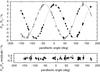 |
Fig. 1 Upper panel: dependence of NTT/EFOSC2 instrumental polarization on parallactic angle. Open and closed symbols refer to the normalized Stokes parameters PQ and PU, respectively. The solid and dashed lines are fits to the PQ and PU data, respectively (Eqs. (1) and (2)). Lower panel: residuals after subtracting the fit. |
After removing the dependence on parallactic angle, we found the instrumental polarization to also depend on the position on the CCD. The instrumental polarization was zero at the center of the CCD and increased to ~0.5% in the corners. The field dependence was modeled by fitting two-dimensional polynomials up to second degree to PQ and PU and removed. After this no significant residuals above the error bars (0.1−0.2%) were seen.
At Calar Alto we examined the polarization of 360 field stars present in the CCD frames. These stars are not necessarily unpolarized, but since they are not at low galactic latitudes, their polarization is expected to be low, below, or close to our error bars (0.05−0.5%). There is a clear dependence of polarization on the position on the CCD (Fig. 2) reaching 3−4% near the corners. As with the NTT data, we fitted up to second-order, two-dimensional polynomials to PQ and PU and subtracted the fit from the data. After subtraction no residuals above the rms noise in PQ and PU (0.2%) were seen.
Statistics of the observed sample.
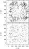 |
Fig. 2 Degree of polarization of field stars with the Calar Alto 2.2 m telescope/CAFOS as a function of position on the CCD before (upper panel) and after (lower panel) applying the corrections. An arrow with a length of 100 units corresponds to 1% polarization. |
The NOT data show no instrumental effects above the rms noise (0.3%) of 26 field stars. We can thus say that any remaining instrumental effects in our whole data set are below 0.2−0.3% in PQ and PU, considerably less than typical error bars in BL Lac candidates (~0.8%).
To determine whether a target is polarized, we computed the 95% confidence limits of the observed degree of polarization P using the formalism in Simmons & Stewart (1985). If the lower confidence limit of P is >0, we denote the target as polarized. In this case the unbiased degree of polarization was computed using the maximum likelihood estimator in Simmons & Stewart (1985); i.e.,  where σP = (σPQ + σPU)/2. If the target was unpolarized (i.e. the lower 95% confidence limit = 0), we used the upper 95% confidence limit as the upper limit for the degree of polarization.
The polarization position angle was calibrated by making 21 observations of six highly polarized stars in Schmidt et al. (1992) and Fossati et al. (2007). We used the quoted R-band values to determine the position angle zero point. The derived zero points have an rms scatter of ~1° internally for each instrument. Since we used filters that are slightly different from the R-band and since the polarization position angle in high polarization standards is typically wavelength-dependent, though not strongly, a small systematic error in our PA calibration was expected. We compared the derived r-band zero points to the ones derived in Villforth et al. (2010) for the R-band and found the two to differ by 1.4 ± 1.3 and by 1.8 ± 1.1 degrees for the CA and NOT data, respectively. As a result, any PA offsets due to filter mismatch are likely to be smaller than 2 degrees.
4. Results
The results for each object individually are presented in Table 1, while we give a breakdown of our results in Table 2 as discussed below.
In total, we have 195 measurements (123 NTT, 47 CA, 25 NOT) of 182 targets. According to C05, 135 out of 182 targets were not reported in NED before they published their sample. Thirteen of our 182 targets were observed twice using the NOT and NTT or CA, and 10 out of 13 were not listed in NED when C05 published their catalog.
Out of our 182 targets 124 (68%) have been found to be polarized and 95 out of the 124 (77%) polarized objects have been found to be highly polarized with P > 4%3. The average polarization is 7%, with a substantial tail of 27 targets whose polarization exceeds 10% and a maximum polarization of 22%. Figure 3 shows the distribution of the polarization degree of our targets. There is basically no difference in the distribution of the “already known” and really new BL Lac candidates. Indeed, a K-S test confirmed that the null hypothesis that the two p distributions are drawn from the same parent population cannot be rejected (significance 0.204). We also inspected the distribution of the polarization angles. As expected we do not find any preferred polarization angle.
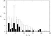 |
Fig. 3 Distribution of the degree of polarization of our targets. The candidates with entries in NED are indicated in black. |
Only 44 out of 124 (35%) of our polarized sources have a reliable redshift, 33 have lower limits and/or uncertain redshifts while for 47 targets no redshift is available at all. The redshifts are taken from the catalog of C05. Their reliable redshifts are based on at least two spectral features (mostly but not always from the host galaxy absorption features), lower limits are derived from intervening absorption systems (typically Mg II), while uncertain redshifts are based on one single spectral feature. Our results clearly indicate the need for deep follow-up spectroscopy.
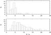 |
Fig. 4 Distribution of the degree of polarization of our 44 targets with reliable redshifts (upper panel) and of our 80 targets with either lower limits, uncertain, or no redshifts at all (lower panel). |
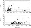 |
Fig. 5 Polarization versus redshift of our targets with reliable redshifts (black dots), lower limits to the redshift (right arrows), and upper limits to the polarization (down arrows). The dashed line marks 4% polarization. The upper panel displays the results for the full data set, while the lower panel shows our results for redshifts up to z = 1 only. |
Figure 4 shows the distribution of the degree of polarization for the 44 BL Lac candidates with reliable redshift and the 80 remaining ones in separate panels. Obviously, the two distributions differ in the sense that the targets with reliable z tend to be less polarized. The median polarization for the targets with reliable redshift is 3.8% and for the remaining ones 7.8%, respectively. A KS-test shows that the two distributions are not different at a < 0.01% level. This results can best be explained by contamination of our polarization measurements by host galaxy light for the sources with reliable redshifts (see above and discussion in Sect. 5.2).
In Fig. 5 we show the behavior of our sources in the polarization-redshift plane. There seems to be a trend toward sources with higher redshifts to be more polarized roughly up to z ~ 1. This would indicate a bias, since at higher redshift only the more beamed sources can be detected and the dilution by host galaxy light is much lower. (Our polarization measurements have not yet been corrected for host galaxy contamination.) Above z ~ 1, the polarization of the sources seems to drop. There is one weakly polarized source at a redshift >3 and a few more sources where we could derive only upper limits. These may be high-redshift weak-line QSOs (see discussion in Sect. 5.3). However, there are potentially five more highly and two more weakly polarized sources above z = 1 in our sample, but their redshifts are marked as uncertain in C05. To test for a correlation of polarization with redshift, we calculated the Spearman rank correlation coefficient for all 43 sources with reliable redshifts up to z = 1. We only find ρ = 0.284. A Student’s T-test confirmed that ρ is not significantly different from 0 (τρ = 1.90). We also tested whether the polarization properties of the 22 low-z (z < 0.35) and the 21 high-z (z > 0.35) sources differ. According to a KS-test, the polarization properties of the two subsamples are not significantly different. The expected bias is not as pronounced as one may expect. This could come from the small apertures for our polarimetry used (see discussion in Sect. 5.2).
All of our 124 polarized sources have a radio detection in either FIRST (faint images of the radio sky at twenty centimeters, Becker et al. 1995) or NVSS (NRAO VLA Sky Survey, Condon et al. 1998), or have recently been detected in deep VLA observations by Plotkin et al. (2010b, P10b hereafter). Only 44 (35%) of our 124 sources are detected in both the radio and X-ray regime. This is not surprising since the X-ray measurements were taken from the RASS (ROSAT All-Sky Survey, e.g. Truemper 1993), which is generally much shallover than the radio surveys used for cross-correlation. Upcoming deep X-ray surveys like the one planned by eRosita will certainly detect a major fraction of the sources discussed here. Nevertheless, most targets that have been found to be polarized are true new “bona fide” BL Lac objects. Only 84 out of 240 sources were listed as BL Lac in NED at the time when C05 published his sample. In the meantime, the number of NED entries is much larger, but this is exclusively due to newly presented samples by A07 and P10a.
Remarkable is the breakdown of our 58 unpolarized sources. Thirtynine of them (67%) have either a radio counterpart (25 sources, with one recently been detected by P10b; SDSS J21155288+000115.5, but still radio-quiet) or a X-ray detection (1 source), or they have been detected in radio and X-rays (13 sources). About 60% (23 out of 39) of them have a reliable redshift.
The 19 unpolarized sources that have been detected neither at radio nor at X-ray frequencies all belong to the potential radio-weak BL Lac candidates presented by C05. Reliable redshifts are available for 42% (8 out of 19) of these sources.
Our data set allows us to inspect some of our targets for polarization variability. Six targets have been observed with a separation of a couple of days (NTT and NOT), seven targets with a separation of about six weeks (CA and NOT), and 21 more targets with a separation of three to four years (our data and S07). A comparison of the polarization measurements taken at different epochs is provided in Fig. 6. As can be seen, a large fraction (~1/3) of our BL Lac candidates show polarization variability indeed. Polarization measurements are available in the literature for six more of our sources. These are the two 1Jy BL Lacs SDSS J005041.31-092905.1 and SDSS J014125.83-092843.7 observed by Brindle et al. (1986) and Mead et al. (1990), the two EMSS BL Lacs SDSS J020106.18+003400.2 and SDSS J140450.91+040202.2 observed by Jannuzi et al. (1994), SDSS J105829.62+013358.8 observed by Impey & Tapia (1988), and SDSS J121834.93-011954.3 observed by Sluse et al. (2005). For all sources polarization between 5% and 30% was detected. Comparing the measurements to ours, all six sources have shown polarization variability on timescales of years.
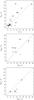 |
Fig. 6 Polarization measurements of S07 compared to ours (top), NOT vs. CA (center) and NOT vs. NTT (bottom). The diagonal line gives the 1:1 correspondence. The arrows indicate upper limits. Polarization variability for a number of objects is apparent in particular at larger baselines. |
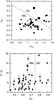 |
Fig. 7 Upper panel: positions of our sources with polarization in the αox − αro plane. The area of the symbol is proportional to the degree of polarization. The division line between HBL and LBL is also indicated. Only the 45 targets with radio and X-ray counterparts are included here. Lower panel: the degree of polarizarion P as a function of αrx. |
5. Discussion and conclusions
5.1. General comments
Although BL Lac objects are by definition polarized, have a duty cycle of at least 40% to be highly polarized (Jannuzi et al. 1993b, 1994), and their polarization properties can be used to probe radiation processes in their central engines (e.g. Valtonen et al. 2008; Villforth et al. 2010; Fermi-Lat Collaboration et al. 2010), polarization measurements have rarely been used to verify them. So far, only Impey & Brand (1982), Borra & Corriveau (1984), Impey & Tapia (1988), Fugmann & Meisenheimer (1988), Kuehr & Schmidt (1990), Jannuzi et al. (1993a), Kock et al. (1996), Marcha et al. (1996), and S07 used polarization measurements as a diagnostic tool for detecting or confirming BL Lac candidates.
About 124 of the 182 targets observed by us were found to be polarized, and 95 were highly polarized. S07 observed 21 more sources not observed by us. All of them were found to be polarized, 15 out of 21 were highly polarized. Since S07 and we concentrated on sources without an entry in NED, it is not a surprise that the majority of the remaining sources are already known BL Lacs, e.g., from the RGB sample by Laurent-Muehleisen et al. (1999). Polarization measurements are published for only eight more sources4, all of which were found to be polarized and five to be highly polarized. In sum, polarization measurements are available for 211 of 240 targets (88%) from the C05 sample of probable BL Lac candidates, 153 (64%) of them were found to be polarized at least once, and 115 (48%) to be highly polarized.
5.2. HBL versus LBL
Figure 7 shows the location of our polarized sources with both radio and X-ray detection in the αox − αro plane as well as the degree of polarizarion P as a function of αrx. As in C05, we use αrx = 0.75 as the dividing line between LBL and HBL. Obviously, more HBL than LBL are in this figure, which may be because the radio surveys (NVSS, FIRST) are much deeper than the X-ray survey (RASS). Although we are limited by low number statistics here, it seems that the HBL are only slightly less polarized on average than LBLs. The average polarization for our eight LBL in the diagram is 8.7 ± 1.9% (mode 6.2%), while it is 5.6 ± 0.6% (mode 5.0%) for the 37 HBL. As “errors” we quote the standard error of the mean. A K-S test confirmed that our LBL and HBL do not show a significantly different polarization (significance 0.0758).
The two most highly polarized LBL are the 1 Jy BL Lac SDSS J005041.31-092905.1 and SDSS J105829.62+013358.8, both of which were found to be highly polarized before. On the other hand, a number of strongly (>10%) polarized sources are HBL, most of them without any entry in NED. The object with the highest polarization in our entire data set (22%, SDSS J121348.81+642520.2), does not enter the plot here since only upper limits to its X-ray flux are available. With αox > 1.07 and αro = 0.43 it is very much in the center of the HBL region. To move it into the LBL region (αox ~ 1.4 for αro = 0.43), its X-ray flux must be a factor 7 below the upper limit in C05.
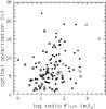 |
Fig. 8 Radio flux versus optical polarization of our SDSS BL Lac candidates. Open squares denote LBL, crossed squares HBL, and dots candidates, where only upper limits to X-ray fluxes exist. Only a weak correlation is apparent. |
Interestingly, 25 of the 37 (68%) HBL that enter Fig. 7 were found to be >4% polarized (and all eight LBL). This seems to be different from the results obtained by Jannuzi et al. (1994), who find a duty cycle (fraction of time spent with P > 4% and assuming that the temporal distribution of polarization is equivalent to the distribution of polarization measured in all objects of its class) for HBL to be only about 44%. Since LBL are stronger radio emitters than HBL, one would not expect any strong correlation between optical polarization and radio flux. As Fig. 8 shows, this is indeed not the case. The Spearman rank-order correlation coefficient rs = 0.31; i.e., the two sets of data only show a weak positive correlation. On the other hand, if we compute an “error” for the duty cycle such that we count the number of objects that could, within their 1σ errors, move above and below the 4% border as in Jannuzi et al. (1994), we find a duty cycle for our HBL of  %. We note that the average redshift of our 15 HBL with reliable redshift is z = 0.37 ± 0.17, which is very similar to the ones obtained for the EMSS or Exosat samples; i.e., there are good reasons to assume that we are dealing with the same class of HBL.
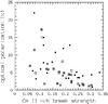 |
Fig. 9 Ca II H/K break strength versus optical polarization for 50 of our BL Lac candidates. The symbols represent the same type of targets as in Fig. 8. The dependence of the degree of polarization on break strength is obvious. HBLs are distributed across the entire break strength range. |
Even within the “error”, we find a higher duty cycle than Jannuzi et al. (1994). There could be several reasons for that. It might be simply a chance coincidence, but could also be an effect of large errors in the derivation of the spectral radio – optical and optical – X-ray indices because the data are not taken simultaneously. Most likely, however, it stems from a combination of the choice of the aperture for measuring the polarimetric fluxes and of the seeing effects. Jannuzi et al. (1994) modeled the change in the measured polarization with respect to the intrinsic polarization as a function of the Ca II H/K break strength in the spectra of BL Lac objects. For a reasonable range of break strengths, they predicted a “depolarization” of up to 20%. In Fig. 9 we show the Ca II H/K break strength versus optical polarization for the 50 targets of our sample (5 LBL, 25 HBL and 20 targets where only upper limits to their X-ray fluxes are available) with the break strengths published in P10a. Obviously, highly polarized sources (P > 4%) can be detected at all break strengths, but the lower the break strength, the higher the measured polarization can be. The diagram basically confirms the prediction by Jannuzi et al. (1994). It shows also that HBL do not necessarily populate the righthand side of the diagram.
Carini et al. (1991), Cellone et al. (2000), and Nilsson et al. (2007) have shown that the choice of the aperture may have a dramatic effect on variability measurements of BL Lac objects due to the presence of the host galaxy. In addition, varying seeing while the apterture is kept constant adds further uncertainties. For their observations Jannuzi et al. (1994) used mostly a two-holer polarimeter/photometer with aperture diameters of 5″or larger (see Table 4 in Jannuzi et al. 1993b). For the majority of our sources, we instead used apertures with a diameter of 4″ or smaller (see Sect. 3). Although our procedure does not completely remove the host galaxy light (see Fig. 9), we expect that the contamination by stellar light is much less in our case. Thus one could expect a higher duty cycle for HBL as the one found by Jannuzi et al. (1994).
To test this, we redid our polarization analysis with a fixed aperture diameter of 5″ similar to the one used by Jannuzi et al. (1994). Compared to our previous analysis, the general result did not change much. Now 116 instead 124 out of 182 sources are polarized (64% instead of 68%), while 88 out of 116 (76%) instead of 95 out of 124 (77%) are highly polarized. Some stronger differences can be seen when we compare the polarization properties of our 8 LBL and 36 HBL. Even with a larger aperture, all LBL are highly polarized. However, of 36 only 29 HBL are polarized and 22 (61%) are highly polarized. When we again compute an “error” for the duty cycle as described above, we now find a duty cycle for our HBL of  %. This is within the “error” very close to the value derived by Jannuzi et al. (1994). We are right now in the process of deblending the polarization measurements of our BL Lac candidates into the contribution of the AGN and host galaxy. Potentially, the polarimetry of “host galaxy free” LBL and HBL will show that their duty cycles do not differ. This will be included in a forthcoming paper.
5.3. Radio-quiet BL Lacs
The existence of radio-quiet BL Lac objects has a long and controversial history. While e.g. Stocke et al. (1990) did not found any in the sample of EMSS BL Lac objects, Londish et al. (2004) potentially found a candidate from the 2QZ BL Lac surcey (Londish et al. 2002). However, as P10b argued, the investigated samples were simply too small to find subsets of rarely radio-quiet BL Lac objects. Alternatively, radio-quiet BL Lac candidates could be low-redshift counterparts of the (also rare) weak-line QSOs (WLQ), first detected by Fan et al. (1999). These objects have several properties similar to BL Lac objects, but they do not show strong radio emission and show very low variability and polarization (Diamond-Stanic et al. 2009). They apparently have an intrinsically weak or absent broad emission line region rather than being diluted by the beamed emission from a relativistic jet (e.g. Shemmer et al. 2009, 2010).
C05 extracted a set of 27 radio-quiet BL Lac candidates out of his probable sample of 240 BL Lac objects (a new set of 86 weak-featured radio-quiet objects has more recently been presented by P10a). We have polarization measurements for 25 out of 27 of them, which are summarized in Table 3. For comparison, the results from S07 are given using our 95% criterion of whether a source is polarized or not and from P10b, who presented new target identifications.
Properties of radio-quiet BL Lac candidates.
All except SDSS J024156.38+004351.6 (weakly polarized with P = 2.6%) and SDSS J024157.37+000944.1 (highly polarized with P = 4.0%, respectively) were found to be unpolarized by us. S07 observed 11 out of 27 candidates and found that three are weakly polarized (SDSS J165806.77+611858.9 with P = 1.0%, SDSS J224749.55+134248.2 with P = 0.8% and SDSS J232428.43+144324.4 with P = 0.9%, respectively) according to our 95% criterion. S07 and we have nine targets in common. Except SDSS J165806.77+611858.9, which S07 found to be polarized, while we could only derive upper limits, the remaining ones did not show any polarization in either case. Altogether S07 and we observed all 27 radio-quiet BL Lac candidates and found four to be weakly polarized and one to be highly polarized. Recently, P10b has examined 20 candidates from C05 via variability measurements using SDSS data, new spectral classifications, proper motions, and new radio and X-ray measurements. They classified three targets as low-redshift WLQ, two as absorbed AGNs, four as stars, two as galaxies, eight as unknown, and only one as radio-loud BL Lac. Our observations confirm that the number of reliable radio-quiet BL Lac objects in the C05 sample must be low. The only highly polarized radio-quiet BL Lac candidate (SDSS J024157.37+000944.1) was classified as radio-loud BL Lac by P10b based on new VLA measurements, while the remaining four weakly polarized radio-quiet BL Lac candidates were classfied as unknown, absorbed AGN or WLQ. As already stated by P10b and a few times in the present paper, besides the lack of reliable spectroscopic redshifts for many targets, deep X-ray observations would be very useful for properly evaluating the contents of the C05 sample.
5.4. Final comments
In summary, we have found that
-
124 out of 182 (68%) of our targets were polarized, and 95 out of the 124 polarized targets (77%) to be highly polarized (>4%).
-
Only 44 out of 124 (35%) of our polarized sources have a reliable redshift. There is a clear need for follow-up high S/N spectroscopy.
-
LBL are on average only slighly more strongly polarized than HBL. We found a higher duty cycle of polarization in HBL (~66% have polarization >4%) than in Jannuzi et al. (1994). This may be due to the different apertures used in the analysis.
-
Our data do not give any evidence for the presence of radio-quiet BL Lac objects in the sample of C05.
By just using our (and S07) polarization measurements, we find strong evidence that the sample selected by C05 indeed contains a large number of bona fide BL Lacs. At least 70% of the sources were found to be polarized. Since even very prominent BL Lacs like OJ 287 are unpolarized from time to time (e.g. Villforth et al. 2010), the number of bona fide BL Lac objects in the sample is presumably even higher. We have further options for testing this result. First of all, BL Lac objects are variable, with LBL and HBL having duty cycles of ~40 and 80%, respectively (Heidt & Wagner 1996, 1998). Since our data were taken through filters similar to the one used by the SDSS, we can look for variability in our targets on timescales of years. In addition, we can use our data to analyze the images for the presence of a core repesenting an AGN and a host galaxy. This would demonstrate that these targets where a host galaxy has been found are extragalactic in nature. Finally, we can use the SDSS and UKIDSS to construct broad-band SEDs of our targets and to elegantly identify stars, which may still contaminate the sample, by their blackbody continuum radiation. All three of the above are in progress. Along with our polarization analysis, we have four diagnostic tools at hand to identify the BL Lac content of the sample of C05. This will be the scope of a forthcoming paper (Nilsson et al., in prep.).
Like all BL Lac samples, the C05 sample seriously suffers from the lack of reliable redshifts, which are a prerequisite for the construction of a lumnosity function of BL Lacs, among other possibilities. It is thus no surprise that BL Lac luminosity functions still suffers from low number statistics (e.g. Padovani et al. 2007). The C05 targets were selected with the requirement of having S/N > 100 over at least one of three 500 Å wide spectral bands in the SDSS spectra. The S/N per resolution element is thus much lower than 100 for many targets. Sbarufatti et al. (2006) has shown that S/N > 100 per resolution element is required for detecting the very faint emission lines and/or host galaxy absorption features. We are now in the process of collecting high S/N spectra for all C05 sources that we found to be polarized and whose redshift is uncertain or unknown. In combination with the results from our analysis, we will then be able to derive the necessary steps towards constructing the first luminosity function of an optically selected sample of BL Lac objects.
“A priori” refers to C05 not cross-correlating his targets with X-ray or radio data bases before he extracted the catalog. In fact, 55 of the C05 BL Lac candidates were spectroscopically targeted by the SDSS due to their radio/X-ray properties. The remaining ones are mainly included in the SDSS spectroscopic database because of their UV excess (see discussion in C05, Sect. 5.5; and Smith et al. 2007, Sect. 2), so the C05 sample is not completely free of biases.
In the following, “listed in NED” refers to “listed as BL Lac in NED” when C05 published their sample.
Following Jannuzi et al. (1993b) we set the border line to distinguish between weakly and highly polarized objects to 4%.
SDSS J081815.99+422245.2 (Kuehr & Schmidt 1990), SDSS J083223.22+491321.0 (Kuehr & Schmidt 1990), SDSS J105837.74+562811.2 (Marcha et al. 1996), SDSS J123131.40+641418.2 (Jannuzi et al. 1993b), SDSS J123739.07+625842.8 (Jannuzi et al. 1993b), SDSS J140923.50+593940.7 (Jannuzi et al. 1993b), SDSS J150947.97+555617.3 (Kock et al. 1996), SDSS J164419.98+454644.4 (Kock et al. 1996).
Acknowledgments
We would like to thank the anonymous referee for constructive and detailed suggestions, that improved the presentation of our results. We would also like to thank the staff at Calar Alto for collecting the excellent data in Service Mode, as well as the staff at the NTT and the NOT for their superb support during the observations. J.H. acknowledges support by the Deutsche Forschungsgemeinschaft (DFG) through grant HE 2712/4-1.
References
- Abazajian, K., Adelman-McCarthy, J. K., Agüeros, M. A., et al. 2004, AJ, 128, 502 [Google Scholar]
- Anderson, S. F., Voges, W., Margon, B., et al. 2003, AJ, 126, 2209 [NASA ADS] [CrossRef] [Google Scholar]
- Anderson, S. F., Margon, B., Voges, W., et al. 2007, AJ, 133, 313 [NASA ADS] [CrossRef] [Google Scholar]
- Angel, J. R. P. 1978, ARA&A, 16, 487 [NASA ADS] [CrossRef] [Google Scholar]
- Becker, R. H., White, R. L., & Helfand, D. J. 1995, ApJ, 450, 559 [NASA ADS] [CrossRef] [Google Scholar]
- Beckmann, V., Engels, D., Bade, N., & Wucknitz, O. 2003, A&A, 401, 927 [NASA ADS] [CrossRef] [EDP Sciences] [Google Scholar]
- Borra, E. F., & Corriveau, G. 1984, ApJ, 276, 449 [NASA ADS] [CrossRef] [Google Scholar]
- Brindle, C., Hough, J. H., Bailey, J. A., Axon, D. J., & Hyland, A. R. 1986, MNRAS, 221, 739 [NASA ADS] [CrossRef] [Google Scholar]
- Carini, M. T., Miller, H. R., Noble, J. C., & Sadun, A. C. 1991, AJ, 101, 1196 [NASA ADS] [CrossRef] [Google Scholar]
- Cellone, S. A., Romero, G. E., & Combi, J. A. 2000, AJ, 119, 1534 [NASA ADS] [CrossRef] [Google Scholar]
- Collinge, M. J., Strauss, M. A., Hall, P. B., et al. 2005, AJ, 129, 2542 [NASA ADS] [CrossRef] [Google Scholar]
- Condon, J. J., Cotton, W. D., Greisen, E. W., et al. 1998, AJ, 115, 1693 [NASA ADS] [CrossRef] [Google Scholar]
- Croom, S. M., Smith, R. J., Boyle, B. J., et al. 2004, MNRAS, 349, 1397 [NASA ADS] [CrossRef] [Google Scholar]
- Diamond-Stanic, A. M., Fan, X., Brandt, W. N., et al. 2009, ApJ, 699, 782 [NASA ADS] [CrossRef] [Google Scholar]
- Fan, X., Strauss, M. A., Gunn, J. E., et al. 1999, ApJ, 526, L57 [NASA ADS] [CrossRef] [PubMed] [Google Scholar]
- Fermi-Lat Collaboration, Members of the 3C 279 Multi-Band Campaign, Abdo, A. A., Ackermann, M., Ajello, M., et al. 2010, Nature, 463, 919 [NASA ADS] [CrossRef] [PubMed] [Google Scholar]
- Fossati, L., Bagnulo, S., Mason, E., & Landi Degl’ Innocenti, E. 2007, in The Future of Photometric, Spectrophotometric and Polarimetric Standardization, ed. C. Sterken, ASP Conf. Ser., 364, 503 [NASA ADS] [Google Scholar]
- Fugmann, W., & Meisenheimer, K. 1988, A&AS, 76, 145 [NASA ADS] [Google Scholar]
- Giommi, P., Piranomonte, S., Perri, M., & Padovani, P. 2005, A&A, 434, 385 [NASA ADS] [CrossRef] [EDP Sciences] [Google Scholar]
- Gunn, J. E., Carr, M., Rockosi, C., et al. 1998, AJ, 116, 3040 [NASA ADS] [CrossRef] [Google Scholar]
- Heidt, J., & Wagner, S. J. 1996, A&A, 305, 42 [NASA ADS] [Google Scholar]
- Heidt, J., & Wagner, S. J. 1998, A&A, 329, 853 [NASA ADS] [Google Scholar]
- Impey, C. D., & Brand, P. W. J. L. 1982, MNRAS, 201, 849 [NASA ADS] [Google Scholar]
- Impey, C. D., & Tapia, S. 1988, ApJ, 333, 666 [NASA ADS] [CrossRef] [Google Scholar]
- Jannuzi, B. T., Green, R. F., & French, H. 1993a, ApJ, 404, 100 [NASA ADS] [CrossRef] [Google Scholar]
- Jannuzi, B. T., Smith, P. S., & Elston, R. 1993b, ApJS, 85, 265 [NASA ADS] [CrossRef] [Google Scholar]
- Jannuzi, B. T., Smith, P. S., & Elston, R. 1994, ApJ, 428, 130 [NASA ADS] [CrossRef] [Google Scholar]
- Kock, A., Meisenheimer, K., Brinkmann, W., Neumann, M., & Siebert, J. 1996, A&A, 307, 745 [NASA ADS] [Google Scholar]
- Kuehr, H., & Schmidt, G. D. 1990, AJ, 99, 1 [NASA ADS] [CrossRef] [Google Scholar]
- Laurent-Muehleisen, S. A., Kollgaard, R. I., Feigelson, E. D., Brinkmann, W., & Siebert, J. 1999, ApJ, 525, 127 [NASA ADS] [CrossRef] [Google Scholar]
- Lawrence, A., Warren, S. J., Almaini, O., et al. 2007, MNRAS, 379, 1599 [NASA ADS] [CrossRef] [MathSciNet] [Google Scholar]
- Londish, D., Croom, S. M., Boyle, B. J., et al. 2002, MNRAS, 334, 941 [NASA ADS] [CrossRef] [Google Scholar]
- Londish, D., Heidt, J., Boyle, B. J., Croom, S. M., & Kedziora-Chudczer, L. 2004, MNRAS, 352, 903 [NASA ADS] [CrossRef] [Google Scholar]
- Londish, D., Croom, S. M., Heidt, J., et al. 2007, MNRAS, 374, 556 [NASA ADS] [CrossRef] [Google Scholar]
- Marcha, M. J. M., Browne, I. W. A., Impey, C. D., & Smith, P. S. 1996, MNRAS, 281, 425 [NASA ADS] [CrossRef] [Google Scholar]
- Mead, A. R. G., Ballard, K. R., Brand, P. W. J. L., et al. 1990, A&AS, 83, 183 [Google Scholar]
- Morris, S. L., Stocke, J. T., Gioia, I. M., et al. 1991, ApJ, 380, 49 [NASA ADS] [CrossRef] [Google Scholar]
- Nesci, R., Sclavi, S., & Massaro, E. 2005, A&A, 434, 895 [NASA ADS] [CrossRef] [EDP Sciences] [Google Scholar]
- Nilsson, K., Pasanen, M., Takalo, L. O., et al. 2007, A&A, 475, 199 [NASA ADS] [CrossRef] [EDP Sciences] [Google Scholar]
- Padovani, P., Giommi, P., Landt, H., & Perlman, E. S. 2007, ApJ, 662, 182 [NASA ADS] [CrossRef] [Google Scholar]
- Perlman, E. S., Stocke, J. T., Schachter, J. F., et al. 1996, ApJS, 104, 251 [NASA ADS] [CrossRef] [Google Scholar]
- Plotkin, R. M., Anderson, S. F., Hall, P. B., et al. 2008, AJ, 135, 2453 [NASA ADS] [CrossRef] [Google Scholar]
- Plotkin, R. M., Anderson, S. F., Brandt, W. N., et al. 2010a, AJ, 139, 390 [NASA ADS] [CrossRef] [Google Scholar]
- Plotkin, R. M., Anderson, S. F., Brandt, W. N., et al. 2010b, ApJ, 721, 562 [NASA ADS] [CrossRef] [Google Scholar]
- Richards, G. T., Myers, A. D., Gray, A. G., et al. 2009, ApJS, 180, 67 [NASA ADS] [CrossRef] [Google Scholar]
- Sbarufatti, B., Treves, A., Falomo, R., et al. 2006, AJ, 132, 1 [NASA ADS] [CrossRef] [Google Scholar]
- Schmidt, G. D., Elston, R., & Lupie, O. L. 1992, AJ, 104, 1563 [NASA ADS] [CrossRef] [Google Scholar]
- Schneider, D. P., Richards, G. T., Hall, P. B., et al. 2010, AJ, 139, 2360 [NASA ADS] [CrossRef] [Google Scholar]
- Shemmer, O., Brandt, W. N., Anderson, S. F., et al. 2009, ApJ, 696, 580 [NASA ADS] [CrossRef] [Google Scholar]
- Shemmer, O., Trakhtenbrot, B., Anderson, S. F., et al. 2010, ApJ, 722, L152 [NASA ADS] [CrossRef] [Google Scholar]
- Simmons, J. F. L., & Stewart, B. G. 1985, A&A, 142, 100 [NASA ADS] [Google Scholar]
- Sluse, D., Hutsemékers, D., Lamy, H., Cabanac, R., & Quintana, H. 2005, A&A, 433, 757 [NASA ADS] [CrossRef] [EDP Sciences] [Google Scholar]
- Smith, P. S., Williams, G. G., Schmidt, G. D., Diamond-Stanic, A. M., & Means, D. L. 2007, ApJ, 663, 118 [NASA ADS] [CrossRef] [Google Scholar]
- Stickel, M., Padovani, P., Urry, C. M., Fried, J. W., & Kuehr, H. 1991, ApJ, 374, 431 [NASA ADS] [CrossRef] [Google Scholar]
- Stocke, J. T., Morris, S. L., Gioia, I., et al. 1990, ApJ, 348, 141 [NASA ADS] [CrossRef] [Google Scholar]
- Stoughton, C., Lupton, R. H., Bernardi, M., et al. 2002, AJ, 123, 485 [NASA ADS] [CrossRef] [Google Scholar]
- Truemper, J. 1993, Science, 260, 1769 [NASA ADS] [CrossRef] [PubMed] [Google Scholar]
- Turnshek, D. A., Bohlin, R. C., Williamson, II, R. L., et al. 1990, AJ, 99, 1243 [NASA ADS] [CrossRef] [Google Scholar]
- Urry, C. M., & Padovani, P. 1995, PASP, 107, 803 [NASA ADS] [CrossRef] [Google Scholar]
- Valtonen, M. J., Lehto, H. J., Nilsson, K., et al. 2008, Nature, 452, 851 [NASA ADS] [CrossRef] [PubMed] [Google Scholar]
- Véron-Cetty, M., & Véron, P. 2010, A&A, 518, A10 [NASA ADS] [CrossRef] [EDP Sciences] [Google Scholar]
- Villforth, C., Nilsson, K., Østensen, R., et al. 2009, MNRAS, 397, 1893 [NASA ADS] [CrossRef] [Google Scholar]
- Villforth, C., Nilsson, K., Heidt, J., et al. 2010, MNRAS, 402, 2087 [NASA ADS] [CrossRef] [Google Scholar]
- York, D. G., Adelman, J., Anderson, Jr., J. E., et al. 2000, AJ, 120, 1579 [Google Scholar]
All Tables
All Figures
|
Fig. 1 Upper panel: dependence of NTT/EFOSC2 instrumental polarization on parallactic angle. Open and closed symbols refer to the normalized Stokes parameters PQ and PU, respectively. The solid and dashed lines are fits to the PQ and PU data, respectively (Eqs. (1) and (2)). Lower panel: residuals after subtracting the fit. |
| In the text | |
|
Fig. 2 Degree of polarization of field stars with the Calar Alto 2.2 m telescope/CAFOS as a function of position on the CCD before (upper panel) and after (lower panel) applying the corrections. An arrow with a length of 100 units corresponds to 1% polarization. |
| In the text | |
|
Fig. 3 Distribution of the degree of polarization of our targets. The candidates with entries in NED are indicated in black. |
| In the text | |
|
Fig. 4 Distribution of the degree of polarization of our 44 targets with reliable redshifts (upper panel) and of our 80 targets with either lower limits, uncertain, or no redshifts at all (lower panel). |
| In the text | |
|
Fig. 5 Polarization versus redshift of our targets with reliable redshifts (black dots), lower limits to the redshift (right arrows), and upper limits to the polarization (down arrows). The dashed line marks 4% polarization. The upper panel displays the results for the full data set, while the lower panel shows our results for redshifts up to z = 1 only. |
| In the text | |
|
Fig. 6 Polarization measurements of S07 compared to ours (top), NOT vs. CA (center) and NOT vs. NTT (bottom). The diagonal line gives the 1:1 correspondence. The arrows indicate upper limits. Polarization variability for a number of objects is apparent in particular at larger baselines. |
| In the text | |
|
Fig. 7 Upper panel: positions of our sources with polarization in the αox − αro plane. The area of the symbol is proportional to the degree of polarization. The division line between HBL and LBL is also indicated. Only the 45 targets with radio and X-ray counterparts are included here. Lower panel: the degree of polarizarion P as a function of αrx. |
| In the text | |
|
Fig. 8 Radio flux versus optical polarization of our SDSS BL Lac candidates. Open squares denote LBL, crossed squares HBL, and dots candidates, where only upper limits to X-ray fluxes exist. Only a weak correlation is apparent. |
| In the text | |
|
Fig. 9 Ca II H/K break strength versus optical polarization for 50 of our BL Lac candidates. The symbols represent the same type of targets as in Fig. 8. The dependence of the degree of polarization on break strength is obvious. HBLs are distributed across the entire break strength range. |
| In the text | |
Current usage metrics show cumulative count of Article Views (full-text article views including HTML views, PDF and ePub downloads, according to the available data) and Abstracts Views on Vision4Press platform.
Data correspond to usage on the plateform after 2015. The current usage metrics is available 48-96 hours after online publication and is updated daily on week days.
Initial download of the metrics may take a while.