| Issue |
A&A
Volume 529, May 2011
|
|
|---|---|---|
| Article Number | A82 | |
| Number of page(s) | 9 | |
| Section | The Sun | |
| DOI | https://doi.org/10.1051/0004-6361/201016326 | |
| Published online | 07 April 2011 | |
Magnetohydrodynamic waves in solar partially ionized plasmas: two-fluid approach
1
Space Research Institute, Austrian Academy of Sciences,
Schmiedlstrasse 6,
8042
Graz,
Austria
e-mail: This email address is being protected from spambots. You need JavaScript enabled to view it.
; This email address is being protected from spambots. You need JavaScript enabled to view it.
; This email address is being protected from spambots. You need JavaScript enabled to view it.
2 Abastumani Astrophysical Observatory at Ilia State
University, Kazbegi ave. 2a, Tbilisi, Georgia
Received:
15
December
2010
Accepted:
5
February
2011
Abstract
Context. Partially ionized plasma is usually described by a single-fluid approach, where the ion-neutral collision effects are expressed by Cowling conductivity in the induction equation. However, the single-fluid approach is not valid for time-scales less than ion-neutral collision time. For these time-scales the two-fluid description is the better approximation.
Aims. We aim to derive the dynamics of magnetohydrodynamic (MHD) waves in two-fluid partially ionized plasmas and to compare the results with those obtained under single-fluid description.
Methods. Two-fluid equations are used, where ion-electron plasma and neutral particles are considered as separate fluids. Dispersion relations of linear waves are derived for the simplest case of homogeneous medium. Frequencies and damping rates of waves are obtained for different parameters of background plasma.
Results. We found that two- and single-fluid descriptions give similar results for low-frequency waves. However, the dynamics of MHD waves in the two-fluid approach is significantly changed when the wave frequency becomes comparable with or higher than the ion-neutral collision frequency. Alfvén and fast magneto-acoustic waves attain their maximum damping rate at particular frequencies (for example, the peak frequency equals 2.5 times the ion-neutral collision frequency for 50% of neutral hydrogen) in the wave spectrum. The damping rates are reduced for the higher frequency waves. The new mode of slow magneto-acoustic wave appears for higher frequency branch, which is connected to neutral hydrogen fluid.
Conclusions. The single-fluid approach perfectly deals with slow processes in partially ionized plasmas, but fails for time-scales shorter than ion-neutral collision time. Therefore, the two-fluid approximation should be used for the description of relatively fast processes. Some results of the single-fluid description should be revised in future such as the damping of high-frequency Alfvén waves in the solar chromosphere due to ion-neutral collisions.
Key words: Sun: atmosphere / Sun: oscillations
© ESO, 2011
1. Introduction
Astrophysical plasmas often are partially ionized. Neutral atoms may change the plasma dynamics through collisions with charged particles. The ion-neutral collisions may lead to different new phenomena in the plasma, for example the damping of magnetohydrodynamic (MHD) waves (Khodachenko et al. 2004; Forteza et al. 2007). The solar photosphere, the chromosphere, and the prominences contain a significant amount of neutral atoms, therefore the complete description of plasma processes requires the consideration of partial ionization effects.
Braginskii (1965) gave the basic principles of transport processes in plasma including the effects of partial ionization. Since this review, numerous papers addressed the problem of partial ionization in the different regions of solar atmosphere. Khodachenko & Zaitsev (2002) studied the formation of the magnetic flux tube in a converging flow of the solar photosphere, while Vranjes et al. (2008) studied the Alfvén waves in weakly ionized photospheric plasma. Leake & Arber (2005) and Arber et al. (2007) studied the effect of partially ionized plasma on emerging magnetic flux tubes and concluded that the chromospheric neutrals may transform the magnetic tube into force-free configuration. Haerendel (1992), De Pontieu & Haerendel (1998), James & Erdélyi (2002), and James et al. (2004) considered the damping of Alfvén waves through ion-neutral collision as a mechanism of spicule formation. Khodachenko el al. (2004) and Leake et al. (2006) studied the importance of ion-neutral collisions in the damping of MHD waves in the chromosphere and prominences. Forteza et al. (2007; 2008), Soler et al. (2009a; 2009b; 2010), and Carbonell et al. (2010) studied the damping of MHD waves in partially ionized prominence plasma with and without plasma flow.
All these papers considered the single-fluid MHD approach when the inertial terms in the momentum equation of the relative velocity between ions and neutrals are neglected. The partially ionized plasma effects are described by a generalized Ohm’s law with Cowling conductivity, which leads to the modified induction equation (Khodachenko el al. 2004). Ambipolar diffusion is more pronounced during the transverse motion of plasma with regard to the magnetic field, therefore the Alfvén and fast magneto-acoustic waves are more efficiently damped. The slow magneto-acoustic waves are weakly damped in the low plasma beta case. Moreover, Forteza et al. (2007) found that the damping rate of slow magneto-acoustic waves derived through a normal mode analysis is different from that estimated by Braginskii (1965). The cause of the discrepancy between the normal mode analysis (Forteza et al. 2007) and the energy consideration (Braginskii 1965) is still an open question, and the present study attempts to shed light on it.
The single-fluid approach has been shown to be valid for the time-scales that are longer than the ion-neutral collision time. However, the approximation fails for the shorter time-scales, therefore the two-fluid approximation, which means the treatment of ion-electron and neutral gases as separate fluids, should be considered. The two-fluid approximation is valid for time-scales longer than the ion-electron collision time, which is significantly shorter because of the Coulomb collision between ions and electrons.
In this paper, we study MHD waves in two-fluid partially ionized plasma. We pay particular attention to the wave damping through ion-neutral collisions and compare the wave dynamics in single and two-fluid approximations. We derive the two-fluid MHD equations from initial three-fluid equations and solve the linearized equations in the simplest case of a homogeneous plasma.
2. Main equations
We aim to study partially ionized plasma, which consists of electrons, ions, and neutral atoms. We assume that each species has a Maxwell velocity distribution, therefore they can be described as separate fluids. Below we first write the equations in three-fluid description and then perform the consequent transition to two-fluid and single-fluid approaches.
2.1. Three-fluid equations
The fluid equations for each species can be derived from Boltzmann kinetic equations,
which have the forms (Braginskii 1965; Goedbloed
& Poedts 2004)![Mathematical equation: \begin{eqnarray} \label{ne3} &&{{\partial n_{\rm e}}\over {\partial t}}+\nabla \cdot (n_{\rm e} \vec V_{\rm e})=0, \\[1.5mm]\label{ni3} &&{{\partial n_{\rm i}}\over {\partial t}}+\nabla \cdot (n_{\rm i} \vec V_{\rm i})=0, \\[1.5mm]\label{nn3} &&{{\partial n_{\rm n}}\over {\partial t}}+\nabla \cdot (n_{\rm n} \vec V_{\rm n})=0, \\ &&m_{\rm e}n_{\rm e}\left ({{\partial \vec V_{\rm e}}\over {\partial t}}+({\vec V_{\rm e}}\cdot \nabla)\vec V_{\rm e}\right )=-\nabla p_{\rm e}-\nabla \cdot \pi_{\rm e} \notag\\\label{Ve3}&&\qquad-en_{\rm e}\left (\vec E +{1\over c}\vec V_{\rm e} \times \vec B \right) +\vec R_{\rm e}, \\[1.5mm] &&m_{\rm i}n_{\rm i}\left ({{\partial \vec V_{\rm i}}\over {\partial t}}+({\vec V_{\rm i}}\cdot \nabla)\vec V_{\rm i}\right )=-\nabla p_{\rm i}-\nabla \cdot \pi_{\rm i}\notag\\\label{Vi3}&&\qquad+Zen_{\rm i}\left (\vec E +{1\over c}\vec V_{\rm i} \times \vec B \right) +\vec R_{\rm i}, \\[1.5mm]\label{Vn3} &&m_{\rm n}n_{\rm n}\left ({{\partial \vec V_{\rm n}}\over {\partial t}}+({\vec V_{\rm n}}\cdot \nabla)\vec V_{\rm n}\right )=-\nabla p_{\rm n}-\nabla \cdot \pi_{\rm n}+\vec R_{\rm n}, \\[1.5mm]\label{Te3} &&{3\over 2}n_{\rm e} k \left ({{\partial T_{\rm e}}\over {\partial t}}\!+\!({\vec V_{\rm e}}\cdot \nabla)T_{\rm e}\right )\!+\!p_{\rm e}\nabla \cdot \vec V_{\rm e}+\pi_{\rm e} \!:\! \nabla \vec V_{\rm e}\!=\!-\nabla \cdot \vec q_{\rm e}+Q_{\rm e}\quad\quad\quad \\[1.5mm]\label{Ti3} &&{3\over 2}n_{\rm i} k \left ({{\partial T_{\rm i}}\over {\partial t}} +({\vec V_{\rm i}}\cdot \nabla)T_{\rm i}\right )+p_{\rm i}\nabla \cdot \vec V_{\rm i}+\pi_{\rm i} : \nabla \vec V_{\rm i}\!=\!-\nabla \cdot \vec q_{\rm i}+Q_{\rm i}\quad\quad\quad \\[1.5mm]\label{Tn3} &&{3\over 2}n_{\rm n} k \left ({{\partial T_{\rm n}}\over {\partial t}} \!+\!({\vec V_{\rm n}}\cdot \nabla)T_{\rm n}\right )\!+\!p_{\rm n}\nabla \cdot \vec V_{\rm n}\!+\!\pi_{\rm n} \!:\! \nabla \vec V_{\rm n}\!=\!-\nabla \cdot \vec q_{\rm n}\!+\!Q_{\rm n}\quad\quad\quad \\[1.5mm]\label{p3} &&p_{\rm e}=n_{\rm e}kT_{\rm e},\,\,p_{\rm i}=n_{\rm i}kT_{\rm i},\,\,p_{\rm n}=n_{\rm n}kT_{\rm n}, \end{eqnarray}](/articles/aa/full_html/2011/05/aa16326-10/aa16326-10-eq2.png) where
ma,
na,
pa,
Ta,
Va are the mass, the
density, the pressure, the temperature and the velocity of particles a,
E is the electric field, B
is the magnetic field strength,
qa is the heat flux density of
particles a, Ra
is the change of impulse of particles a through collisions with other
sort of particles, Qa is the heat production
through collisions of particles a with other sort of particles,
πa is the off-diagonal pressure tensor of
particles a, e = 4.8 × 10⁻¹⁰ statcoul is the
electron charge, c = 2.9979 × 1010 cm s-1 is the
speed of light and k = 1.38 × 10⁻¹⁶ erg K-1 is the
Boltzmann constant. The double dot indicates that a double sum over the Cartesian
components is to be taken. The plasma is supposed to be quasi-neutral, which means
ne = Zni. Below
we consider hydrogen ions and hydrogen neutral atoms that imply Z = 1.
The description of the system is completed by Maxwell equations, which have the forms
(without displacement current)
where
ma,
na,
pa,
Ta,
Va are the mass, the
density, the pressure, the temperature and the velocity of particles a,
E is the electric field, B
is the magnetic field strength,
qa is the heat flux density of
particles a, Ra
is the change of impulse of particles a through collisions with other
sort of particles, Qa is the heat production
through collisions of particles a with other sort of particles,
πa is the off-diagonal pressure tensor of
particles a, e = 4.8 × 10⁻¹⁰ statcoul is the
electron charge, c = 2.9979 × 1010 cm s-1 is the
speed of light and k = 1.38 × 10⁻¹⁶ erg K-1 is the
Boltzmann constant. The double dot indicates that a double sum over the Cartesian
components is to be taken. The plasma is supposed to be quasi-neutral, which means
ne = Zni. Below
we consider hydrogen ions and hydrogen neutral atoms that imply Z = 1.
The description of the system is completed by Maxwell equations, which have the forms
(without displacement current) ![Mathematical equation: \begin{eqnarray} \label{e} &&\nabla \times \vec E=-{1\over c}{{\partial \vec B}\over {\partial t}}, \\[2.2mm]\label{B} &&\nabla \times \vec B={{4 \pi} \over c}{\vec j}, \end{eqnarray}](/articles/aa/full_html/2011/05/aa16326-10/aa16326-10-eq21.png) where
where
 (13)is the
current density.
(13)is the
current density.
For a Maxwell distribution in each species,
Ra and
Qa are expressed as (Braginskii 1965): ![Mathematical equation: \begin{eqnarray} \label{Re} &&\vec R_{\rm e}=-\alpha_{\rm ei}(\vec V_{\rm e}-\vec V_{\rm i})-\alpha_{\rm en}(\vec V_{\rm e}-\vec V_{\rm n}), \\[2.5mm]\label{Ri} &&\vec R_{\rm i}=-\alpha_{\rm ie}(\vec V_{\rm i}-\vec V_{\rm e})-\alpha_{\rm in}(\vec V_{\rm i}-\vec V_{\rm n}), \\[2.5mm]\label{Rn} &&\vec R_{\rm n}=-\alpha_{\rm ne}(\vec V_{\rm n}-\vec V_{\rm e})-\alpha_{\rm ni}(\vec V_{\rm n}-\vec V_{\rm i}), \\[2.5mm]\label{Qe} &&Q_{\rm e}=\alpha_{\rm ei}(\vec V_{\rm e}-\vec V_{\rm i})\vec V_{\rm e}+\alpha_{\rm en}(\vec V_{\rm e}-\vec V_{\rm n})\vec V_{\rm e}, \\[2.5mm]\label{Qi} &&Q_{\rm i}=\alpha_{\rm ie}(\vec V_{\rm i}-\vec V_{\rm e})\vec V_{\rm i}+\alpha_{\rm in}(\vec V_{\rm i}-\vec V_{\rm n})\vec V_{\rm i}, \\[2.5mm]\label{Qn} &&Q_{\rm n}=\alpha_{\rm ne}(\vec V_{\rm n}-\vec V_{\rm e})\vec V_{\rm n}+\alpha_{\rm ni}(\vec V_{\rm n}-\vec V_{\rm i})\vec V_{\rm n}, \end{eqnarray}](/articles/aa/full_html/2011/05/aa16326-10/aa16326-10-eq23.png) where
αab = αba
are the coefficients of friction between particles a and
b.
where
αab = αba
are the coefficients of friction between particles a and
b.
For time-scales longer than the ion-electron collision time, the electron and ion gases can be considered as a single fluid. This significantly simplifies the equations, taking into account the smallness of electron mass with regard to the masses of ion and neutral atoms. Then the three-fluid description can be changed to the two-fluid description, where one component is the ion-electron gas and the second component is the gas of neutral atoms.
2.2. Two-fluid equations
Summing of Eqs. (4) and (5), Eqs. (7) and (8), and first
two equations of Eq. (10), we obtain (after
neglecting the electron inertia and the viscosity effect expressed by the off-diagonal
pressure tensor πa) 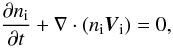 (20)
(20) where
pie = pi + pe
is the pressure of ion-electron gas and
γ = Cp/Cv = 5/3
is the ratio of specific heats.
where
pie = pi + pe
is the pressure of ion-electron gas and
γ = Cp/Cv = 5/3
is the ratio of specific heats.
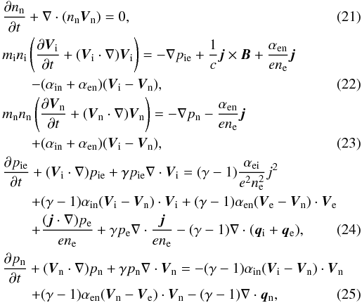
Ohm’s law is obtained from the electron equation (Eq. (4)) after neglecting the electron inertia (i.e. the left-hand side
terms) and it has the form 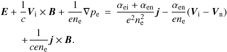 (26)The
Maxwell equation (Eq. (11)) and Ohm’s law
(Eq. (26)) lead to the induction equation
(26)The
Maxwell equation (Eq. (11)) and Ohm’s law
(Eq. (26)) lead to the induction equation
 (27)where
 (28)is
the coefficient of the magnetic diffusion.
(28)is
the coefficient of the magnetic diffusion.
The coefficient of friction between ions and neutrals (if they have the same temperature)
is calculated as (Braginskii 1965)  (29)where
min = mimn/(mi + mn)
is the reduced mass and
(29)where
min = mimn/(mi + mn)
is the reduced mass and  is the
collision cross section between ions and neutrals.
is the
collision cross section between ions and neutrals.
The collision frequency between ions and neutrals is then 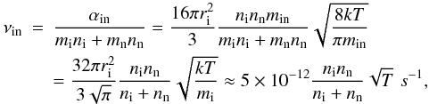 (30)where
the atomic cross section
(30)where
the atomic cross section  cm2
is used and T is normalized by 1 K. The chromospheric
temperature of 104 K and hydrogen ion and neutral number densities of
2.3 × 1010 cm-3 and 1.2 × 1010 cm-3
(Fontenla et al. 1990, model FAL-3) give the
collision frequency as 4 s-1.
cm2
is used and T is normalized by 1 K. The chromospheric
temperature of 104 K and hydrogen ion and neutral number densities of
2.3 × 1010 cm-3 and 1.2 × 1010 cm-3
(Fontenla et al. 1990, model FAL-3) give the
collision frequency as 4 s-1.
For time-scales longer than ion-neutral collision time (1/νin), the system can be considered as a single fluid (the full equations of single-fluid MHD including neutral hydrogen are presented in Appendix A). However, when the time-scales are near to or shorter than the ion-neutral collision time, the single-fluid description is not valid and the two-fluid equations should be considered. Below, in what follows we study the linear MHD waves in a two-fluid description.
3. Linear MHD waves
We consider the simplest case of static and homogeneous plasma with a homogeneous
unperturbed magnetic field. Then the linearized two-fluid equations following from Eqs.
(20)–(25) and (27) are
(neglecting the Hall term and the collision between neutrals and electrons i.e.
αen ≪ αin)  where
where
 (
( ) are perturbations of
the ion (neutral) density, vi
(vn) are the perturbations of ion (neutral)
velocity,
) are perturbations of
the ion (neutral) density, vi
(vn) are the perturbations of ion (neutral)
velocity,  (
( ) are the
perturbations of ion-electron (neutral) gas pressure, b is the
perturbation of the magnetic field, and
ρi0 = mini0,ρn0 = mnnn0,pie,pn,B0
are their unperturbed values, respectively. Equations (31)–(32) and Eqs. (36)–(37) lead to the expressions
) are the
perturbations of ion-electron (neutral) gas pressure, b is the
perturbation of the magnetic field, and
ρi0 = mini0,ρn0 = mnnn0,pie,pn,B0
are their unperturbed values, respectively. Equations (31)–(32) and Eqs. (36)–(37) lead to the expressions  (38)where
 and
and  are the sound speeds of ion-electron and neutral gases, respectively.
Below we consider the unperturbed magnetic field, Bz, directed along the z axis and the wave propagation in xz plane i.e. ∂/∂y = 0. Then Eqs. (31)–(37) can be split into Alfvén and magneto-acoustic waves.
3.1. Alfvén waves
Let us assume that the Alfvén waves are polarized along y axis. We
intend to study the damping of Alfvén waves through the collision between ions and
neutrals. Therefore, we neglect the magnetic diffusion for simplicity. Then, Eqs. (31)–(37) give 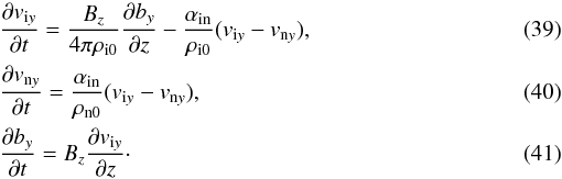
Fourier analyses assuming disturbances to be proportional to exp [i(kzz − ωt)] give the dispersion relation
 (42)where
 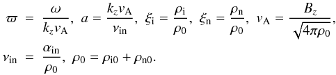 (43)The
same dispersion relation can be obtained from linear single-fluid equations by retaining
the inertial term in Eq. (A.6). The
dispersion relation of the Alfvén waves in linear single-fluid equations without the
inertial term can be easily derived as
(43)The
same dispersion relation can be obtained from linear single-fluid equations by retaining
the inertial term in Eq. (A.6). The
dispersion relation of the Alfvén waves in linear single-fluid equations without the
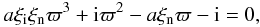
inertial term can be easily derived as 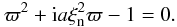 (44)The solution of
Eq. (44) is
(44)The solution of
Eq. (44) is 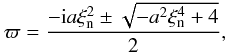 (45)which for
 gives the damping rate
 (46)in full
coincidence with Braginskii (1965). In contrast, the
condition
(46)in full
coincidence with Braginskii (1965). In contrast, the
condition  in Eq. (46) retains only the imaginary part, which
gives the cut-off wave number
in Eq. (46) retains only the imaginary part, which
gives the cut-off wave number  (47)The value of the cut-off
wave number has been obtained recently by Barcélo et al. (2010). Hence, the waves with a higher wave number than
kc are evanescent. However, it might be an incomplete
conclusion because the complete treatment requires the inclusion of inertial terms, and
therefore dealing with Eq. (42) instead of
Eq. (44). The first term in Eq. (42) is important for the high-frequency part
of the wave spectrum and could not be neglected. We demonstrate it by the solutions of
Eqs. (44) and (42).
(47)The value of the cut-off
wave number has been obtained recently by Barcélo et al. (2010). Hence, the waves with a higher wave number than
kc are evanescent. However, it might be an incomplete
conclusion because the complete treatment requires the inclusion of inertial terms, and
therefore dealing with Eq. (42) instead of
Eq. (44). The first term in Eq. (42) is important for the high-frequency part
of the wave spectrum and could not be neglected. We demonstrate it by the solutions of
Eqs. (44) and (42).
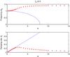 |
Fig. 1 Alfvén wave frequency vs. normalized wave number. The top (bottom) panel shows the real (imaginary) part of the normalized frequency ϖ = ω/kzvA vs. the normalized wavenumber a = kzvA/νin. The blue line corresponds to the solution of the single-fluid dispersion relation, i.e. Eq. (44) and red asterisks are the solutions of the two-fluid dispersion relation, Eq. (42). The values are calculated for 50% of neutral hydrogen, ξn = 0.5. |
Figure 1 displays the solutions of the single-fluid (Eq. (44), blue lines) and two-fluid (Eq. (42), red asterisks) dispersion relations for ξn = 0.5. We see that the frequencies and damping rates of Alfvén waves are the same in the single-fluid and two-fluid approaches for the low-frequency branch of the spectrum (small a). But the behavior is dramatically changed when the wave frequency becomes comparable with or higher than the ion-neutral collision frequency, νin, i.e. for a > 1. The damping time linearly increases with a and the wave frequency becomes zero at some point in the single-fluid case (blue lines). The point where the wave frequency becomes zero corresponds to the cut-off wave number kc of Barcélo et al. (2010). However, there is no cut-off wave number in solutions of two-fluid dispersion relation (red asterisks): Eq. (42) always has a solution with a real part. Therefore, the occurrence of the cut-off wave number in the single-fluid description is the result of neglecting the inertial terms in the momentum equation of relative velocity between ions and neutrals. Therefore, Eq. (42) is the correct dispersion relation for the whole spectrum of waves. But the dispersion relation (44) is still a good approximation for the lower frequency part of spectrum. Another interesting point of the two-fluid approach is that the damping rate (i.e. ωI) attains its maximal value at some wave-lengths for which a ≈ 2.5. The damping rate decreases for smaller and larger a. This means that the waves, which have the frequency in the interval νin < ω < 10 νin, have stronger damping than other harmonics of the spectrum. This is totally different from the single-fluid solutions, which show the linear increase of damping rate with increasing wave number (lower panel, blue line).
Figure 2 displays the same solutions as in the Fig. 1, but for ξn = 0.1. The solutions have basically the same properties as those with ξn = 0.5. However, the wave length with the maximal damping rate is now shifted to a ≈ 10.
3.2. Magneto-acoustic waves
Now let us turn to magneto-acoustic waves. We consider the waves and wave vectors
polarized in xz plane. Then Eqs. (31)–(37) are written
as (magnetic diffusion is again neglected) 
A Fourier analysis with
exp [i(kxx + kzz − ωt)]
and some algebra give the dispersion relation ![Mathematical equation: \begin{eqnarray} &&\nu^2_{\rm in} \omega\left [\omega^4-k^2 (c^2_{\rm si} \xi_{\rm i} + c^2_{\rm sn} \xi_{\rm n} + V^2_{\rm A}) \omega^2+(c^2_{\rm si}\xi_{\rm i} + c^2_{\rm sn} \xi_{\rm n}) k^2 k^2_z V^2_{\rm A} \right ] \notag\\ &&-\xi_{\rm i} \xi^2_{\rm n} \omega (\omega^2-c^2_{\rm sn} k^2) \left [\xi_{\rm i} \omega^4-k^2 V^2_{\rm A} \omega^2 +c^2_{\rm si} k^2 (k^2_z V^2_{\rm A} - \xi_{\rm i} \omega^2)\right ] \notag\\ &&-{\rm i} \nu_{\rm in} \xi_{\rm n} [(\xi_{\rm n}-2) k^2 V^2_{\rm A} \omega^4 +2 \xi_{\rm i} \omega^6 +c^2_{\rm sn} k^2 \omega^2 \left (k^2 V^2_{\rm A} + (\xi^2_{\rm n}-1)\omega^2 \right ) \notag\\\label{disp-mhd} &&+c^2_{\rm si} \xi_{\rm i} k^2 \left (2 k^2_z V^2_{\rm A} \omega^2 + (\xi_{\rm n}-2) \omega^4 + c^2_{\rm sn} k^2 (\omega^2-k^2_z V^2_{\rm A}) \right )]=0, \arraycolsep1.75pt \end{eqnarray}](/articles/aa/full_html/2011/05/aa16326-10/aa16326-10-eq89.png) (57)where
(57)where
 .
.
The dispersion relation (57) is a seventh
order equation with ω, therefore it has seven different solutions. For
smaller wave numbers (or lower frequencies) four of the solutions represent the usual
magneto-acoustic waves, while three other solutions are purely imaginary and are probably
connected to the vortex modes (with Re(ω) = 0) that damped through ion
neutral collisions. The vortex modes are solutions of fluid equations and they correspond
to the fluid vorticity. The vortex modes have zero frequency in the ideal fluid, but may
gain a purely imaginary frequency if dissipative processes are evolved. The two vortex
modes are transformed into oscillatory modes for shorter wavelengths (see the next
paragraph). Then we have two fast magneto-acoustic modes, four slow magneto-acoustic
modes, and one vortex solution with a purely imaginary part. Below we consider that the
temperatures of all three species are equal i.e.
Ti = Te = Tn,
which gives  .
.
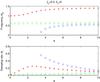 |
Fig. 3 Frequency and damping rate of different wave modes in two-fluid MHD vs. the normalized wavenumber a = kzvA/νin. Frequencies and damping rates are normalized by kvA. Red asterisks correspond to the fast magneto-acoustic mode and green diamonds correspond to the usual slow magneto-acoustic mode. The mode with the blue squares is the new sort of slow magneto-acoustic wave (“neutral” slow mode), which arises for larger wave numbers. This mode has only an imaginary frequency for small wave numbers, which is not shown in this figure. Frequencies and damping rates are calculated for the waves propagating along the magnetic field. The neutral hydrogen is taken to be 50% (ξn = 0.5). Here we consider csn/vA = 0.5. |
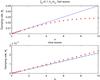 |
Fig. 4 Damping rate of the fast (upper panel) and slow (lower panel) magneto-acoustic waves, i.e. with the imaginary part of ω normalized by kvA, vs. the normalized wavenumber a = kzvA/νin. The blue solid lines correspond to the solution of the single-fluid dispersion relation and the dashed line corresponds to the slow magneto-acoustic damping rate of Braginskii (the expressions used are from Forteza et al. 2007). Red asterisks are the solutions of the two-fluid dispersion relation, Eq. (57). The values are calculated for 10% of neutral hydrogen, ξn = 0.1, and for csn/vA = 0.1. The damping rates are calculated for waves propagating with a 45° angle with regard to the magnetic field. |
Figure 3 displays all oscillatory solutions of the two-fluid dispersion relation for ξn = 0.5 (only the modes with positive frequencies are shown). The wave propagation is parallel to the magnetic field and we use csn/vA = 0.5, where csn is the sound speed of neutral hydrogen. For smaller wave numbers, k < 3.5 νin/vA, there are two normal magneto-acoustic modes, fast (red asterisks) and slow (green diamonds). However, for larger wave-numbers, k > 3.5 νin/vA one additional sort of slow magneto-acoustic mode with a strong damping rate (blue squares) arises. The “neutral” slow mode is connected with neutral atoms. For the higher frequency range, i.e. for a higher than ion-neutral collision frequency, the neutral gas does not feel the ions, therefore it supports the propagation of the additional oscillatory wave mode. This mode obviously disappears for lower frequencies because the collisions couple ions and neutrals and they behave as a single fluid. In other words, for lower frequencies (or small wave numbers) this mode has a zero real part, but a non-zero imaginary part (not shown in the figure). Therefore, the more correct statement is that the oscillatory mode transforms into non-oscillatory vortex mode for smaller wave numbers. The fast magneto-acoustic modes decouple from the slow waves for the parallel propagation and show the same behavior as Alfvén waves. Therefore, the plot of fast magneto-acoustic waves is similar to that of Alfvén waves (see Fig. 1).
It is useful to compare the solutions of two-fluid dispersion relation with those obtained in the single-fluid approach. The damping of fast and slow magneto-acoustic waves has been derived from the energy equation by Braginskii (1965), Khodachenko et al. (2004), Khodachenko & Rucker (2005), and through a normal mode analysis by Forteza et al. (2007). Damping rates are the same in both considerations for fast magneto-acoustic waves, but they disagree for slow magneto-acoustic waves (Forteza et al. 2007). Namely, slow magneto-acoustic waves show damping for purely parallel propagation in the case of Braginskii, while the damping is absent in Forteza et al. (2007). Our Figs. 4 and 5 show the damping rates of fast and slow magneto-acoustic waves vs. a (i.e. k) for the propagation angles of 45° and 0°, respectively. Red asterisks are the solutions of the two-fluid dispersion relation – Eq. (57). The blue solid lines correspond to the solutions of the single-fluid dispersion relation from Forteza et al. (2007). The dashed line corresponds to the slow magneto-acoustic damping rate of Braginskii (1965). Here we use csn/vA = 0.1 so the plasma β is small enough. The neutral hydrogen concentration is taken to be 10%. The fast magneto-acoustic waves have essentially the same dynamics as the Alfvén waves. For the smaller wave numbers (or lower frequencies) the two-fluid and single-fluid approaches give the same results, but for the larger wave numbers the damping rate is decreased in the two-fluid description as in the case of Alfvén waves. In contrast, the slow magneto-acoustic waves have similar damping rates in both approaches. There is a small discrepancy between the damping rates for the waves propagating with 45° degree about the magnetic field, but all three cases (two-fluid waves, single-fluid waves, and energy consideration) yield similar results. The parallel propagation reveals an interesting result: the two-fluid solutions are exactly the same as those obtained by Braginskii (the damping rate obtained by Forteza et al. 2007 is zero for the parallel propagation). Therefore, the discrepancy between the damping rates of the slow magneto-acoustic waves obtained by Forteza et al. 2007) and Braginskii (1965) is again caused by neglecting the inertial terms in the momentum equation of relative velocity (Eq. (A.6)). Braginskii (1965) used the energy equation to calculate the damping rate, therefore his solution agrees with that obtained in our two-fluid approach.
Figure 6 shows the comparison of the damping rates in the two-fluid approach and those obtained by Braginskii (1965) for ξn = 0.5, csn/vA = 0.1 and parallel propagation. The fast magneto-acoustic waves have the same behavior as the Alfvén waves (see lower panel of Fig. 1), which is significantly different from Braginskii (1965) and Forteza et al. (2007). But the slow magneto-acoustic waves have the same damping rate as those of Braginskii (1965). On the other hand, the damping rate of slow magneto-acoustic waves becomes different from the solution of Braginskii (1965) for higher plasma β. Figure 7 shows the same as Fig. 6, but for csn/vA = 0.5. The damping rate of the slow magneto-acoustic waves now begins to deviate from the solution of Braginskii for higher wave numbers. The behavior of fast magneto-acoustic waves remains the same.
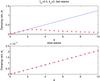 |
Fig. 6 Damping rate (the imaginary part of the normalized frequency ϖ = ω/kzvA) of fast (upper panel) and slow (lower panel) magneto-acoustic waves vs. the normalized wavenumber a = kzvA/νin. Red asterisks are the solutions of the two-fluid dispersion relation. Blue lines correspond to the solutions of Braginskii. The values are calculated for 50% of neutral hydrogen and csn/vA = 0.1. The damping rates are calculated for the waves that propagate along the magnetic field. |
4. Discussion
Some parts of the solar atmosphere contain a large number of neutral atoms: most of the atoms are neutral at the photospheric level, but the ionization degree rapidly increases with height owing to the increased temperature. Solar prominences also contain neutral atoms. Neutral atoms may change the dynamics of the plasma through collision with charged particles. For time-scales longer than the ion-neutral collision time, the partially ionized plasma can be considered as one fluid, because collisions between neutrals and charged particles lead to the rapid coupling of the two fluids. Then the equation of motion is written for the center-of-mass velocity, and the motion of the species is considered as diffusion with a low velocity compared with the velocity of the center-of-mass. The corresponding collision terms appear in the equation of motion for the relative velocity (between ions and neutrals) and in the generalized Ohm’s law. Neglecting the inertial term in the equation of motion for the relative velocity, one simplifies the equations, and a traditional induction equation with Cowling conductivity is obtained (Braginskii 1965; Khodachenko et al. 2004). The inertial terms (left-hand side terms in Eq. (A.6)) are smaller than the collision term (the last term in the same equation), but become comparable for time-scales near the ion-neutral collision time. Therefore, it can be neglected only for longer time-scales.
But for the time-scales of less than the ion-neutral collision time, both fluids may behave independently and the single-fluid approximation is not valid any more. Accordingly the two-fluid approximation, when ion-electron and neutral atom gases are treated as separate fluids, should be considered when one tries to model the processes in partially ionized plasmas.
The normal mode analysis of the two-fluid partially ionized plasma shows that frequencies and damping rates of low-frequency MHD waves agree well with those found in the single-fluid approach. However, the waves with higher frequency than the ion-neutral collision frequency show a significantly different behavior. Alfvén and fast magneto-acoustic waves have maximal damping rates in a particular frequency interval, which peaks, for example, at the frequency ω = 2.5 νin, (νin is the ion-neutral collision frequency) for ξn = 0.5 and at the frequency ω = 10 νin for ξn = 0.1. The damping rates are reduced for the higher frequency part of wave spectrum (note that the damping rates are linearly increased in the single-fluid approach). Therefore, the statements concerning the damping of high-frequency Alfvén waves in the solar chromosphere through ion-neutral collisions should be revised. A careful analysis is needed to study the damping of high-frequency Alfvén waves for a realistic height profile of the ionization degree in the chromosphere.
Another important point concerning the Alfvén waves in partially ionized plasma is the cut-off wave-number, which appears in the single-fluid approach (Barcélo et al. 2010). Barcélo et al. (2010) found that the Alfvén waves with larger wave numbers than the cut-off value are evanescent in partially ionized and resistive plasmas. However, our two-fluid analysis shows that there is no cut-off wave number owing to ambipolar diffusion (see Fig.1, red asterisks). Therefore, the appearance of a cut-off wave number in the single-fluid approach is the result of neglecting of the inertial term in the equation of motion for the relative velocity. It is possible that the cut-off wave number that arises because of an usual magnetic resistivity is caused by neglecting the electron inertia, therefore the cut-off may completely disappear in a three-fluid approach. The cut-off wave numbers also appear for fast magneto-acoustic waves in partially ionized and resistive plasmas (Barcélo et al. 2010). We suggest that this may also be caused by neglecting the inertial term. However, this point needs further study.
The two-fluid approach reveals two different slow magneto-acoustic modes when the slow wave time-scale becomes shorter than the ion-neutral collision time (Fig. 3). The different slow modes correspond to ion-electron and neutral fluids. But only one slow magneto-acoustic mode remains at the lower frequency range as in the commonly used single-fluid approach. This is easy to understand physically. If the wave frequency is lower than the ion-neutral collision frequency, the two fluids are coupled through collisions and only one slow magneto-acoustic wave appears. The mode connected with the neutral fluid (“neutral” slow mode) has only an imaginary frequency in this range of the wave spectrum (not shown in Fig. 3). This means that any slow wave-type change (density, pressure) in the neutral fluid is damped faster than the wave period owing to collisions with ions. The “neutral” slow magneto-acoustic wave has similar properties as the ion magneto-acoustic waves.
The two-fluid approach of partially ionized plasma clarifies the uncertainty concerning the damping rate of slow magneto-acoustic waves found in the single-fluid approach. We found that the normal mode analysis and energy consideration method (used by Braginskii 1965) leads to different expressions for the damping rate of slow waves (Forteza et al. 2007). We found that the damping rate obtained in the two-fluid approach agrees well with the damping rate of Braginskii, which is derived from the energy treatment (see lower panels of Figs. 5–6). Therefore, it seems that the discrepancy is again caused by neglecting the inertial terms in the equation of motion for the relative velocity in the single-fluid approach. Braginskii (1965) used the general energy method for the estimation of damping rates, and this is probably the reason why his results agree with those found in the two-fluid approach.
Here we have considered only neutral hydrogen as a component of partially ionized plasma. However, other neutral atoms, for example neutral helium, may have important effects in the MHD wave damping processes. Soler et al. (2010) made the first attempt to include the neutral helium in the single-fluid description of prominence plasma. They concluded that the neutral helium has no significant influence on the damping of MHD waves. However, the two-fluid approach may give some more details about the effects of neutral helium on MHD waves, therefore it is important to study this point in the future.
5. Conclusions
Frequencies and damping rates of low-frequency MHD waves in the two-fluid description are similar to those obtained in the single-fluid approach. But high-frequency waves (with a higher frequency than the ion-neutral collision frequency) have a completely different behavior.
Alfvén and fast magneto-acoustic waves have maximal damping rates at some frequency interval that peaks at a particular frequency. The peak frequency is 2.5 νin, where νin is the ion-neutral collision frequency, for 50% of neutral hydrogen. For 10% of neutral hydrogen, the peak frequency is shifted to10 νin. The damping rate is reduced for higher frequencies, therefore the damping of high-frequency Alfvén waves in the solar chromosphere with a realistic height profile of the ionization degree needs to be revised in future.
There are two types of slow magneto-acoustic waves in the high-frequency part of the wave spectrum: one connected with the ion-electron fluid and another with the fluid of neutrals.
There is no cut-off frequency of Alfvén waves because of ambipolar diffusion. The cut-off frequency found in the single-fluid approach is caused by neglecting the inertial terms in the momentum equation of relative velocity.
The damping rate of slow magneto-acoustic waves is similar to Braginksii (1965) in low plasma β approximation. The deviation from the Braginskii formula found by the normal mode analysis in the single-fluid approach (Forteza et al. 2007) is probably caused by neglecting the inertial terms.
Acknowledgments
The work was supported by the Austrian Fonds zur Förderung der wissenschaftlichen Forschung (project P21197-N16). T.V.Z. also acknowledges financial support from the Georgian National Science Foundation (under grant GNSF/ST09/4-310).
References
- Arber, T. D., Haynes, M., & Leake, J. E. 2007, ApJ, 666, 541 [NASA ADS] [CrossRef] [Google Scholar]
- Barcélo, S., Carbonell, M., & Ballester, J. L. 2010, A&A, 525, A60 [Google Scholar]
- Braginskii, S. I. 1965, Rev. Plasma Phys., 1, 205 [NASA ADS] [Google Scholar]
- Carbonell, M., Forteza, P., Oliver, R., & Ballester, J. L. 2010, A&A, 515, A80 [NASA ADS] [CrossRef] [EDP Sciences] [Google Scholar]
- De Pontieu, B., & Haerendel, G. 1998, A&A, 338, 729 [NASA ADS] [Google Scholar]
- Fontenla, J. M., Avrett, E. H., & Loeser, R. 1990, ApJ, 355, 700 [NASA ADS] [CrossRef] [Google Scholar]
- Forteza, P., Oliver, R., Ballester, J. L., & Khodachenko, M. L. 2007, A&A, 461, 731 [NASA ADS] [CrossRef] [EDP Sciences] [Google Scholar]
- Forteza, P., Oliver, R., & Ballester, J. L. 2008, A&A, 492, 223 [NASA ADS] [CrossRef] [EDP Sciences] [Google Scholar]
- Goedbloed, H., & Poedts, S. 2004, Principles of Magnetohydrodynamics (Cambridge University Press) [Google Scholar]
- Khodachenko, M. L., & Rucker, H. O. 2005, Adv. Space Res., 36, 1561 [NASA ADS] [CrossRef] [Google Scholar]
- Khodachenko, M. L., & Zaitsev, V. V. 2002, Astrophys. Space Sci., 279, 389 [NASA ADS] [CrossRef] [Google Scholar]
- Khodachenko, M. L., Arber, T. D., Rucker, H. O., & Hanslmeier, A. 2004, A&A, 422, 1073 [NASA ADS] [CrossRef] [EDP Sciences] [Google Scholar]
- Haerendel, G. 1992, Nature, 360, 241 [NASA ADS] [CrossRef] [Google Scholar]
- James, S. P., & Erdélyi, R. 2002, A&A, 393, L11 [NASA ADS] [CrossRef] [EDP Sciences] [Google Scholar]
- James, S. P., Erdélyi, R., & De Pontieu, B. 2004, A&A, 406, 715 [Google Scholar]
- Leake, J. E., & Arber, T. D. 2006, A&A, 450, 805 [NASA ADS] [CrossRef] [EDP Sciences] [Google Scholar]
- Leake, J. E., Arber, T. D., & Khodachenko, M. L. 2005, A&A, 442, 1091 [NASA ADS] [CrossRef] [EDP Sciences] [Google Scholar]
- Soler, R., Oliver, R., & Ballester, J. L. 2009a, ApJ, 699, 1553 [NASA ADS] [CrossRef] [Google Scholar]
- Soler, R., Oliver, R., & Ballester, J. L. 2009b, ApJ, 707, 662 [NASA ADS] [CrossRef] [Google Scholar]
- Soler, R., Oliver, R., & Ballester, J. L. 2010, A&A, 512, A28 [NASA ADS] [CrossRef] [EDP Sciences] [Google Scholar]
- Vranjes, J., Poedts, S., Pandey, B. P., & de Pontieu, B. 2008, A&A, 478, 553 [NASA ADS] [CrossRef] [EDP Sciences] [Google Scholar]
Appendix A: Single-fluid equations
We use the total velocity (i.e. velocity of center of mass)  (A.1)the
relative velocity
(A.1)the
relative velocity  (A.2)and the total density
 (A.3)Equation (20)–(25) and (27) lead to the system
![Mathematical equation: \appendix \setcounter{section}{1} \begin{eqnarray} \label{n1} &&{{\partial \rho}\over {\partial t}}+\nabla \cdot (\rho \vec V)=0, \\[2mm]\label{V1b} &&\rho{{\partial \vec V}\over {\partial t}}+\rho({\vec V}\cdot \nabla)\vec V=-\nabla p+{1\over c}\vec j \times \vec B - \nabla \cdot (\xi_{\rm i} \xi_{\rm n} \rho \vec w \vec w), \end{eqnarray}](/articles/aa/full_html/2011/05/aa16326-10/aa16326-10-eq115.png)
![Mathematical equation: \appendix \setcounter{section}{1} \begin{eqnarray} &&{{\partial \vec w}\over {\partial t}}+({\vec V}\cdot \nabla)\vec w+({\vec w}\cdot \nabla)\vec V+\xi_{\rm n}({\vec w}\cdot \nabla)\vec w-({\vec w}\cdot \nabla)\xi_{\rm i} \vec w \notag\\[2mm]\label{w1} &&=-\left ({{\nabla p_{\rm ie}}\over {\rho \xi_{\rm i}}}-{{\nabla p_{\rm n}}\over {\rho \xi_{\rm n}}}\right )+{1\over {c \rho \xi_{\rm i}}}\vec j \times \vec B+{{\alpha_{\rm en}}\over {e n_{\rm e} \rho \xi_{\rm i} \xi_{\rm n}}}\vec j -{{\alpha_{\rm n}}\over {\rho \xi_{\rm i} \xi_{\rm n}}}\vec w, \\[2mm] &&{{\partial p}\over {\partial t}}+ ({\vec V}\cdot \nabla)p + \gamma p \nabla \cdot \vec V -\xi_{\rm i}({\vec w}\cdot \nabla)p -\gamma p \nabla \cdot (\xi_{\rm i} \vec w) \notag\\[2mm] &&+({\vec w}\cdot \nabla)p_{\rm ie}+\gamma p_{\rm ie} \nabla \cdot \vec w=(\gamma -1) {{\alpha_{\rm ei}+\alpha_{\rm en}}\over {e^2 n^2_{\rm e}}}j^2 +(\gamma -1)\alpha_{\rm n}w^2 \notag\\[2mm] &&-(\gamma -1){{2 \alpha_{\rm en}}\over {e n_{\rm e}}}\vec j \vec w +{1\over {e n_{\rm e}}}({\vec j}\cdot \nabla)p_{\rm e}+ \gamma p_{\rm e}\nabla \cdot {{\vec j}\over {e n_{\rm e}}} \notag\\[2mm]\label{p1} &&-(\gamma -1)\nabla \cdot ({\vec q_{\rm i}}+{\vec q_{\rm e}}+{\vec q_{\rm n}}), \\[2mm] &&{{\partial \vec B}\over {\partial t}}={\nabla \times}(\vec V \times \vec B)+ {\nabla \times}\left ({{c \nabla p_{\rm e}}\over {e n_{\rm e}}}\right )-{\nabla \times}\left (\eta \nabla \times \vec B\right ) \notag\\[2mm]\label{B1} &&\,-{\nabla \times}\left ({{\vec j\times \vec B}\over {en_{\rm e}}}\right )+{\nabla \times}\left ({{c \alpha_{\rm en}\vec w}\over {e n_{\rm e}}}\right )+ {\nabla \times}\left (\xi_{\rm n}\vec w \times \vec B\right ), \end{eqnarray}](/articles/aa/full_html/2011/05/aa16326-10/aa16326-10-eq116.png) where
p = pe + pi + pn,
ξi = ρi/ρ,
ξn = ρn/ρ and
αn = αin + αen.
where
p = pe + pi + pn,
ξi = ρi/ρ,
ξn = ρn/ρ and
αn = αin + αen.
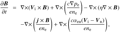
Ohm’s law is now ![Mathematical equation: \appendix \setcounter{section}{1} \begin{eqnarray} &&\vec E + {1\over c}\vec V \times \vec B+ {{1}\over {e n_{\rm e}}}\nabla p_{\rm e}={{\alpha_{\rm ei}+\alpha_{\rm en}}\over {e^2 n^2_{\rm e}}}\vec j-{{\alpha_{\rm en}}\over {e n_{\rm e}}}\vec w +{1\over {cen_{\rm e}}}\vec j\times \vec B \notag\\[2mm]\label{om1} &&-{\xi_{\rm n}\over c}\vec w \times \vec B. \end{eqnarray}](/articles/aa/full_html/2011/05/aa16326-10/aa16326-10-eq121.png) (A.9)Neglecting
the inertia terms, i.e. all left hand side terms in Eq. (A.6), we have
(A.9)Neglecting
the inertia terms, i.e. all left hand side terms in Eq. (A.6), we have
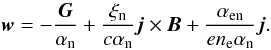 Then the
induction equation takes the form
Then the
induction equation takes the form ![Mathematical equation: \appendix \setcounter{section}{1} \begin{eqnarray} {{\partial \vec B}\over {\partial t}}&=&{\nabla \times}(\vec V \times \vec B)+ {c\over e}{\nabla \times}\left ({{\nabla p_{\rm e} -\epsilon \vec G}\over {n_{\rm e}}}\right )-{\nabla \times}\left (\eta_T \nabla \times \vec B\right ) \notag\\[2mm] &&-{c\over {4 \pi e}}{\nabla \times}\left ({{1-2\epsilon \xi_{\rm n}}\over {n_{\rm e}}}(\nabla \times \vec B)\times \vec B\right ) - {\nabla \times}\left ({{\xi_{\rm n}}\over {\alpha_{\rm n}}}\vec G \times \vec B\right ) \notag\\[2mm]\label{B1b} &&+{\nabla \times}\left ({{\xi^2_{\rm n}}\over {4 \pi \alpha_{\rm n}}}((\nabla \times \vec B)\times \vec B)\times \vec B\right ), \end{eqnarray}](/articles/aa/full_html/2011/05/aa16326-10/aa16326-10-eq123.png) (A.10)where
ϵ = αen/αn,
G = ξn∇pei − ξi∇pn
and
(A.10)where
ϵ = αen/αn,
G = ξn∇pei − ξi∇pn
and 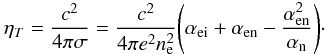 (A.11)These equations are
traditionally used for the description of partially ionized plasmas.
(A.11)These equations are
traditionally used for the description of partially ionized plasmas.
All Figures
|
Fig. 1 Alfvén wave frequency vs. normalized wave number. The top (bottom) panel shows the real (imaginary) part of the normalized frequency ϖ = ω/kzvA vs. the normalized wavenumber a = kzvA/νin. The blue line corresponds to the solution of the single-fluid dispersion relation, i.e. Eq. (44) and red asterisks are the solutions of the two-fluid dispersion relation, Eq. (42). The values are calculated for 50% of neutral hydrogen, ξn = 0.5. |
| In the text | |
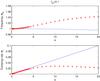 |
Fig. 2 Same as in Fig. 1, but for 10% of neutral hydrogen, ξn = 0.1. |
| In the text | |
|
Fig. 3 Frequency and damping rate of different wave modes in two-fluid MHD vs. the normalized wavenumber a = kzvA/νin. Frequencies and damping rates are normalized by kvA. Red asterisks correspond to the fast magneto-acoustic mode and green diamonds correspond to the usual slow magneto-acoustic mode. The mode with the blue squares is the new sort of slow magneto-acoustic wave (“neutral” slow mode), which arises for larger wave numbers. This mode has only an imaginary frequency for small wave numbers, which is not shown in this figure. Frequencies and damping rates are calculated for the waves propagating along the magnetic field. The neutral hydrogen is taken to be 50% (ξn = 0.5). Here we consider csn/vA = 0.5. |
| In the text | |
|
Fig. 4 Damping rate of the fast (upper panel) and slow (lower panel) magneto-acoustic waves, i.e. with the imaginary part of ω normalized by kvA, vs. the normalized wavenumber a = kzvA/νin. The blue solid lines correspond to the solution of the single-fluid dispersion relation and the dashed line corresponds to the slow magneto-acoustic damping rate of Braginskii (the expressions used are from Forteza et al. 2007). Red asterisks are the solutions of the two-fluid dispersion relation, Eq. (57). The values are calculated for 10% of neutral hydrogen, ξn = 0.1, and for csn/vA = 0.1. The damping rates are calculated for waves propagating with a 45° angle with regard to the magnetic field. |
| In the text | |
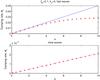 |
Fig. 5 The same as in Fig. 4 but for the parallel propagation, i.e. kx = 0. |
| In the text | |
|
Fig. 6 Damping rate (the imaginary part of the normalized frequency ϖ = ω/kzvA) of fast (upper panel) and slow (lower panel) magneto-acoustic waves vs. the normalized wavenumber a = kzvA/νin. Red asterisks are the solutions of the two-fluid dispersion relation. Blue lines correspond to the solutions of Braginskii. The values are calculated for 50% of neutral hydrogen and csn/vA = 0.1. The damping rates are calculated for the waves that propagate along the magnetic field. |
| In the text | |
 |
Fig. 7 The same as in Fig. 6, but for csn/vA = 0.5. |
| In the text | |
Current usage metrics show cumulative count of Article Views (full-text article views including HTML views, PDF and ePub downloads, according to the available data) and Abstracts Views on Vision4Press platform.
Data correspond to usage on the plateform after 2015. The current usage metrics is available 48-96 hours after online publication and is updated daily on week days.
Initial download of the metrics may take a while.