| Issue |
A&A
Volume 528, April 2011
|
|
|---|---|---|
| Article Number | A52 | |
| Number of page(s) | 6 | |
| Section | Cosmology (including clusters of galaxies) | |
| DOI | https://doi.org/10.1051/0004-6361/201015766 | |
| Published online | 28 February 2011 | |
Estimate of dark halo ellipticity by lensing flexion
1
Argelander-Institut für Astronomie, Universität Bonn,
Auf dem Hügel 71,
53121
Bonn,
Germany
This email address is being protected from spambots. You need JavaScript enabled to view it.
; This email address is being protected from spambots. You need JavaScript enabled to view it.
2
International Max Planck Research School (IMPRS) for Astronomy and
Astrophysics, Auf dem Hügel
69, 53121
Bonn,
Germany
Received:
16
September
2010
Accepted:
28
January
2011
Abstract
Aims. The predictions of the ellipticity of dark matter halos from models of structure formation are notoriously difficult to test with observations. A direct measurement would give important constraints on the formation of galaxies, and its effect on the dark matter distribution in their halos. Here we show that galaxy-galaxy flexion provides a direct and potentially powerful method for determining the ellipticity of (an ensemble of) elliptical lenses.
Methods. We decompose the spin-1 flexion into a radial and a tangential component. Using the ratio of tangential-to-radial flexion, which is independent of the radial mass profile, the mass ellipticity can be estimated.
Results. An estimator for the ellipticity of the mass distribution is derived and tested with simulations. We show that the estimator is slightly biased. We quantify this bias, and provide a method to reduce it. Furthermore, a parametric fitting of the flexion ratio and orientation provides another estimate for the dark halo ellipticity, which is more accurate for individual lenses. Overall, galaxy-galaxy flexion appears as a powerful tool for constraining the ellipticity of mass distributions.
Key words: dark matter / gravitational lensing: weak / galaxies: halos
© ESO, 2011
1. Introduction
The structure of cluster and galaxy halos predicted by N-body simulations of cold dark matter show several important features, e.g. the universal radial density profile (Navarro et al. 1996, 1997), and the highly non-spherical structure fitted well by a triaxial density profile (Jing & Suto 2002; Law et al. 2009). These features are related to the nature of dark matter as well as to the formation of galaxies and clusters (Kuhlen et al. 2007; Debattista et al. 2008; Bett et al. 2010), which suggest that accurate estimates of the halo properties can provide several constraints on cosmology. In particular, numerical simulations with different assumptions predict halos with different shapes, e.g., simulations with non-interacting cold dark matter predict that halos are triaxial prolate ellipsoids (Allgood et al. 2006). Moreover, if there exists a significant difference between the shape of a galaxy and the shape of its total mass distribution, this would provide additional strong evidence for the existence of dark matter (Suyu & Halkola 2010). In other words, it allows us to test how reliable the light is as a tracer of the matter distribution.
Gravitational lensing provides a powerful tool for studying the mass distribution of clusters of galaxies as well as galaxy halos (see Bartelmann & Schneider 2001; Refregier 2003; Schneider et al. 2006; Munshi et al. 2008, for reviews on weak lensing). This is because gravitational lensing probes the matter distribution regardless of whether it is luminous or dark. The weak lensing technique has been used for cluster mass reconstructions (e.g. Clowe et al. 2006; Bradač et al. 2008), and for the ellipticity of the dark matter distribution (Corless et al. 2009; Deb et al. 2010; Howell & Brainerd 2010). A method to determine galaxy halo ellipticity by stacking galaxies was proposed in Natarajan & Refregier (2000) and has been used to determine the ellipticities of both cluster- or galaxy-size halos (Evans & Bridle 2009; Mandelbaum et al. 2006). A mean ellipticity of 0.46 is found from a sample of 25 clusters using Subaru data (Oguri et al. 2010).
Flexion has been recently studied as the derivative of the shear, and responds to small-scale variations in the gravitational potential (Goldberg & Natarajan 2002; Goldberg & Bacon 2005; Bacon et al. 2006). Different techniques were developed to measure flexion (Irwin & Shmakova 2006; Okura et al. 2007; Massey et al. 2007; Schneider & Er 2008). It was noted that flexion can contribute to studies of the dark matter halos in galaxies and clusters, especially for the detection of mass substructure (Bacon et al. 2010; Er et al. 2010). Flexion has been implemented on small sets of observational data. Okura et al. (2008) performed flexion measurement on data from the Subaru telescope to detect substructure in Abell 1689. Leonard et al. (2007) analyzed images taken by the HST Advanced Camera for Surveys, from which a preliminary galaxy-galaxy flexion signal has been detected. Hawken & Bridle (2009) studied galaxy halo ellipticity using flexion. It is found that the constrains from flexion are comparable to, or even tighter than those from shear. Moreover, since flexion drops off faster than the shear as one goes away from the center of the lens, multiple deflections from the three-dimensional mass distribution between us and distant source galaxies (Howell & Brainerd 2010) may not be significant for flexion.
In this paper, we present a new approach to estimate dark matter halo ellipticity using galaxy-galaxy lensing flexion. The spin-1 flexion, a vector, is decomposed into its two components, the radial and tangential flexion. The tangential-to-radial flexion ratio yields an estimate of dark halo ellipticity. We need to assume that the center of the galaxy or the cluster be known. Whereas for galaxies this may be a lesser problem, the mass centroid of clusters is sometimes difficult to determine. We study the effect of noise coming from an intrinsic flexion. In Sect. 3, we perform a series of numerical tests of our estimate and study how our results are biased by the distribution of background sources, the centroid offsets and intrinsic flexion. We discuss our results in Sect. 4.
2. Basic formalism
The full formalism described here can be found in Bacon et al. (2006); Schneider & Er (2008). Weak lensing shear and flexion are conveniently described using a complex notation. We adopt the thin lens approximation, assuming that the lensing mass distribution is projected onto the lens plane. The dimensionless projected mass density can be written as κ(θ) = Σ(θ)/Σcr, where θ is the angular position, Σ(θ) is the projected mass density, and Σcr is the critical surface mass density.
The first-order image distortion by gravitational lensing is described by the shear
γ, which transforms a round source into an elliptical image. The
higher-order effect, which is called flexion, is described by two parameters. The spin-1
flexion is the complex derivative of
κ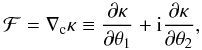 (1)and the spin-3 flexion is
the complex derivative of γ,
(1)and the spin-3 flexion is
the complex derivative of γ,
 (2)
(2)
2.1. Radial and tangential flexion
The spin-1 flexion is a vector-like quantity, the gradient of the surface mass density. Therefore, the spin-1 flexion is directed towards the center of the lens in the case of an axi-symmetric mass distribution. However, if the lens deviates from axial symmetry, e.g., due to elliptical halos or mass substructure (Bacon et al. 2010; Hawken & Bridle 2009), the flexion vector will have a different direction.
In galaxy-galaxy lensing, shear can be decomposed into tangential and cross components.
Analogously, we decompose the spin-1 flexion into a radial and tangential flexion
component. They are defined as  where
the spin-1 flexion vector is given by
ℱ = (ℱ1,ℱ2) = ∇κ in
Cartesian coordinates.
where
the spin-1 flexion vector is given by
ℱ = (ℱ1,ℱ2) = ∇κ in
Cartesian coordinates.  and
and  are the unit direction vectors in polar coordinates. For the spin-3 flexion, there is no
such a clear intuitive picture of its two components; thus, we only consider the spin-1
flexion in this paper.
are the unit direction vectors in polar coordinates. For the spin-3 flexion, there is no
such a clear intuitive picture of its two components; thus, we only consider the spin-1
flexion in this paper.
As mentioned before, the spin-1 flexion vector is not directed towards the center of an elliptical lens (Fig.1). Therefore, the tangential flexion no longer vanishes and can be used to estimate the ellipticity of the mass distribution.
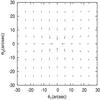 |
Fig. 1 Spin-1 flexion vector field for an elliptical isothermal density distribution with ϵ = 0.3. ℱ only points towards the center when the background galaxy is located on the major or minor axis of the halo. Note that the length of the vectors are logarithmically scaled, for better visibility. |
2.2. Elliptical mass distributions
We now assume that the isodensity contours of the mass distribution are ellipses with
ellipticity ϵ, or equivalently, axis ratio
(1 − ϵ)/(1 + ϵ), and orientation
φ0 of the major axis. In this case, the surface mass density
can be written as 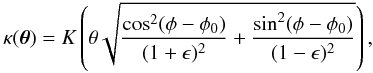 (5)where the function
K(ρ) describes the radial density profile. The
derivatives of κ with respect to radial and azimuthal coordinates are
given as
(5)where the function
K(ρ) describes the radial density profile. The
derivatives of κ with respect to radial and azimuthal coordinates are
given as 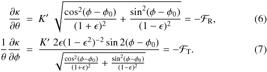 Both
of these derivates have the same radial profile, given by K′. We now
define the flexion ratio as
Both
of these derivates have the same radial profile, given by K′. We now
define the flexion ratio as  (8)which is the tangent of
the angle between the direction to the mass center and the direction of the flexion
vector. For an elliptical mass distribution, this becomes
(8)which is the tangent of
the angle between the direction to the mass center and the direction of the flexion
vector. For an elliptical mass distribution, this becomes  (9)Thus, the flexion ratio
r(φ) depends only on the ellipticity
ϵ and the orientation φ0 of the mass
distribution, not on its radial profile. In particular, it is independent of the lens
strength, and thus of the source and lens redshift. In principle, from the measurement of
the flexion ratio at two polar positions φ, one can determine both
ϵ and φ0, though due to noise, this
determination will have large uncertainty. Alternatively, one can consider the flexion
ratio averaged over all polar angles,
(9)Thus, the flexion ratio
r(φ) depends only on the ellipticity
ϵ and the orientation φ0 of the mass
distribution, not on its radial profile. In particular, it is independent of the lens
strength, and thus of the source and lens redshift. In principle, from the measurement of
the flexion ratio at two polar positions φ, one can determine both
ϵ and φ0, though due to noise, this
determination will have large uncertainty. Alternatively, one can consider the flexion
ratio averaged over all polar angles,  (10)which
depends solely on the ellipticity ϵ. Due to its simplicity, this mean
flexion ratio can be easily measured from a flexion field in a given aperture.
(10)which
depends solely on the ellipticity ϵ. Due to its simplicity, this mean
flexion ratio can be easily measured from a flexion field in a given aperture.
However, we have to assume to know the center of the lens for calculating the two flexion components. For a galaxy, the center is assumed to be the bright center of galaxy. For clusters, the location of the BCG not necessarily coincides with the mass center. Moreover, ‘intrinsic flexion’ also introduces extra noise (see below).
For a given value of ϵ, the flexion ratio is bounded. One can see from
(9) that  (11)Arbitrary large
ellipticities, which would allow r to become very large, are implausible
and most likely do not exist. We can take limits on ϵ from other
observations, e.g., Parker et al. (2007) compared
galaxy-galaxy lensing along the major and minor axes, and found that the axis ratio
b/a of galaxy halos lies between 0.5 and 0.8
(ϵ ∈ [0.11,0.33]). Moreover, Oguri
et al. (2010) analyzed 25 clusters and found
⟨ 1 − b/a ⟩ = 0.46, corresponding to
ϵ = 0.32. Here we use the conservative assumption that
ϵ < 0.8, putting an upper bound to the flexion ratio of
r < 4.5. We will employ this limit to remove excessively large
flexion ratios which are due to noise.
(11)Arbitrary large
ellipticities, which would allow r to become very large, are implausible
and most likely do not exist. We can take limits on ϵ from other
observations, e.g., Parker et al. (2007) compared
galaxy-galaxy lensing along the major and minor axes, and found that the axis ratio
b/a of galaxy halos lies between 0.5 and 0.8
(ϵ ∈ [0.11,0.33]). Moreover, Oguri
et al. (2010) analyzed 25 clusters and found
⟨ 1 − b/a ⟩ = 0.46, corresponding to
ϵ = 0.32. Here we use the conservative assumption that
ϵ < 0.8, putting an upper bound to the flexion ratio of
r < 4.5. We will employ this limit to remove excessively large
flexion ratios which are due to noise.
3. Numerical test with NIE toy model
In this section we describe some simulations which we have performed in order to test the
behavior of the estimator given in the previous section. For this, we model the surface mass
density profile by a non-singular isothermal elliptical profile (NIE), described by
 (12)where
θE is the Einstein radius, describing the strength of the
lens, and θc is the core radius; for
θc = 0, this specializes to the singular isothermal elliptical
profile (SIE). In our simulations, we take θE = 6′′ and
θc = 2′′. Galaxies are randomly distributed within an 1′ × 1′
‘source plane’ behind the lens. Resulting images are discarded if they are located closer to
the halo center than 6′′ (the strong lensing regime) or at distances
|θ| > 30′′, where the flexion signal will be
very small. Moreover, very large flexions cannot be measured (Schneider & Er 2008), thus images with |ℱ| > 0.5 are
discarded as well.
(12)where
θE is the Einstein radius, describing the strength of the
lens, and θc is the core radius; for
θc = 0, this specializes to the singular isothermal elliptical
profile (SIE). In our simulations, we take θE = 6′′ and
θc = 2′′. Galaxies are randomly distributed within an 1′ × 1′
‘source plane’ behind the lens. Resulting images are discarded if they are located closer to
the halo center than 6′′ (the strong lensing regime) or at distances
|θ| > 30′′, where the flexion signal will be
very small. Moreover, very large flexions cannot be measured (Schneider & Er 2008), thus images with |ℱ| > 0.5 are
discarded as well.
The flexion ratio is calculated according to Eq. (8) for each point. A mean flexion ratio is obtained by  (13)where N is
the number of images for each realization. Then the mass ellipticity is estimated, according
to Eq. (10), as
(13)where N is
the number of images for each realization. Then the mass ellipticity is estimated, according
to Eq. (10), as  (14)
(14)
3.1. Noise-free case
Due to the non-linearity, the estimator (14) is expected to be biased. In order to test this, we generated mock data sets with different ϵ = 0.03i, i = 1,2,...20. For each ellipticity, we used 20 realizations, with a density of flexion points of 80 arcmin-2. The filtering described above leads to 63 flexion data for each realization on average.
For each realization, we calculated  from Eq. (13) and estimate
ϵ using Eq. (14). In
Fig.2, we show
from Eq. (13) and estimate
ϵ using Eq. (14). In
Fig.2, we show
 vs. the input value of ϵ. The solid line shows the identity, the plus
points are the estimates from the 20 realizations. In fact, the estimates
closely trace the input value. The variance between different realizations becomes larger
with increasing ϵ. The mean over the 20 realizations is shown by the plus
points in Fig.3, showing that
very slightly underestimates the input value.
vs. the input value of ϵ. The solid line shows the identity, the plus
points are the estimates from the 20 realizations. In fact, the estimates
closely trace the input value. The variance between different realizations becomes larger
with increasing ϵ. The mean over the 20 realizations is shown by the plus
points in Fig.3, showing that
very slightly underestimates the input value.
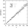 |
Fig. 2 Comparison of the ellipticity estimator (14) with the input ellipticity (solid line). The estimated ellipticity for 20 realizations each for 20 input values of ϵ are shown by pluses, for NIE models with θc = 2′′. |
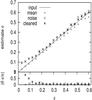 |
Fig. 3 Top panel: comparison of the input ellipticity (solid line) and the estimate (similar as Fig. 2). The plus points show the average estimate for 20 realizations without noise. The other are the result from data with intrinsic noise. All the result are calculated from Eq. (14). The stars are calculated when flexion ratios higher than the upper limit (Eq. (11)) are excluded. Bottom panel: fractional error |δϵ/ϵ| of our estimate for the respective cases. |
3.2. Intrinsic flexion
Our main source of noise is intrinsic flexion, meaning that the sources can have non-vanishing third-order brightness moments. Depending on the method of flexion measurement, the intrinsic noise may be different (Goldberg & Leonard 2007). Since flexion has the dimension of an inverse length, the intrinsic flexion is also inversely proportional to the image size. Therefore, the distribution of intrinsic flexion depends on the survey and is difficult to obtain from real measurements on current data. Effects of a point spread function (PSF) need to be considered, which is far more difficult for flexion than for shear measurements. In particular, an anisotropic PSF may affect the direction of the flexion vector.
We use a simple model to generate intrinsic noise for our simulated data, by setting ℱobs = ℱ1 + nf1 + i(ℱ2 + nf2). The components of the intrinsic flexion nf1,nf2 are drawn from a Gaussian distribution, with each component being characterized by σℱ1 = σℱ2 = 0.03 arcsec-1. This is slightly larger than the intrinsic scatter found by (Goldberg & Leonard 2007), σa |ℱ| = 0.03. On the other hand, (Okura et al. 2008) found a larger scatter in their measurement, σℱ = 0.11 arcsec-1. This is however obtained from a massive galaxy cluster, thus may not be suitable for our galaxy-galaxy lensing flexion.
In Fig.3 we compare the estimates
with the input values (solid line). The plus points show the mean over 20 realizations
without noise (Fig.2), and the dashed line displays
estimates with intrinsic noise included. Not surprisingly, our estimates from noisy
simulations are larger than the input values (intrinsic noise will cause the estimate to
deviate from zero even for a perfectly symmetric mass distribution). This is particularly
significant for small ϵ. As an additional test, we reject flexion data
which have r > 4.5, and perform our estimate again. The mean
result is shown by crosses in Fig.3. One can see that
the bias is slightly reduced in this case, in particular for larger ϵ,
but still
overestimates the true ellipticity. The amplitude of this bias depends of course on the
intrinsic flexion distribution. In Fig.4, we show our
estimate as a histogram of 20 noisy realizations for a halo with
ϵ = 0.57. The dashed histogram corresponds to rejecting the flexion data
with r > 4.5. One can see that the number of overestimates is
reduced.
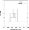 |
Fig. 4 Histogram of the estimated ellipticity for a halo with ϵ = 0.57 from 20 realizations. The solid line is obtained from noise data, the dashed line is the result after excluding the high flexion ratio points. |
Another way to estimate the ellipticity of the mass distribution is to fit the flexion
ratio with the model (9), with the two free
parameters ϵ and φ0. The result for two
realizations is presented in Fig.6. The points are
calculated from simulated data of an NIE with ϵ = 0.3 (left) and
ϵ = 0.6 (right). The dotted lines are the fitting result with
Eq. (9) whereas the solid curves show
Eq. (9) with the input ellipticity. The
fits almost perfectly agree with the input model. For the left panel, the fitting yields
ϵ = 0.31 and φ0 = 0.1, whereas
 .
In the right panel, ϵ = 0.62 and φ0 = 0.006
from fitting, whereas
.
In the right panel, ϵ = 0.62 and φ0 = 0.006
from fitting, whereas  .
In both panels of Fig.6, there are several points
with significant deviations from the fitting curves which is the reason for
to be larger than the input value, whereas these points do not strongly affect the fitting
result.
.
In both panels of Fig.6, there are several points
with significant deviations from the fitting curves which is the reason for
to be larger than the input value, whereas these points do not strongly affect the fitting
result.
Obviously, the fitting method yields a more accurate estimate of the mass ellipticity
than the estimator  ,
and at the same time also estimates the orientation. It is therefore the preferred method
for individual lenses. In contrast, the estimator
can be applied also to an ensemble of lenses, by superposing their respective flexion
values. In this way,
estimates the weighted mean ellipticity of the ensemble of lenses. Note that in contrast
to galaxy-galaxy lensing with the shear method, the individual lenses do not have to be
aligned before the averaging; hence, no assumption about the relative orientation of mass
and light needs to be made.
,
and at the same time also estimates the orientation. It is therefore the preferred method
for individual lenses. In contrast, the estimator
can be applied also to an ensemble of lenses, by superposing their respective flexion
values. In this way,
estimates the weighted mean ellipticity of the ensemble of lenses. Note that in contrast
to galaxy-galaxy lensing with the shear method, the individual lenses do not have to be
aligned before the averaging; hence, no assumption about the relative orientation of mass
and light needs to be made.
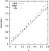 |
Fig. 5 Comparison of mean estimator and biweight estimator. The plus point are the result using mean estimate The crosses are the result using biweight center estimate Eq. (15) to calculate ⟨ r ⟩ . |
3.3. Biweight estimator
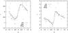 |
Fig. 6 The flexion ratio r varies with φ. The dashed line is for an SIE halo model. The points are calculated from the simulated data, the dotted line is the fit to the results with Eq. (9). Left is a halo with ϵ = 0.3, and right is ϵ = 0.6. |
The assumption that the flexion noise is Gaussian may not be valid, due to the low number
density of background galaxies and the flexion measurement. Thus we adopt as an
alternative estimator the biweight location estimator, which was studied by Beers et al. (1990) as a possible improvement for
non-Gaussian or contaminated normal distributions, 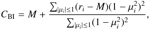 (15)where M
is the sample median and the μi are given by
(15)where M
is the sample median and the μi are given by
 (16)with
 (17)where
ri is the flexion ratio of each galaxy
image. We perform an additional test for the mean and CBI
estimator. In Fig.5, the plus points are the result
when we use
to calculate ⟨ r ⟩ , the cross points are the result from using
CBI. One can see that the bias is reduced significantly.
Moreover, the bias reduction of CBI is independent of halo
ellipticity.
(17)where
ri is the flexion ratio of each galaxy
image. We perform an additional test for the mean and CBI
estimator. In Fig.5, the plus points are the result
when we use
to calculate ⟨ r ⟩ , the cross points are the result from using
CBI. One can see that the bias is reduced significantly.
Moreover, the bias reduction of CBI is independent of halo
ellipticity.
3.4. Centroid offset test
Since the ellipticity represents the deviation from symmetry of a mass distribution, a centroid offset will affect the determination of the ellipticity, leading to an additional bias. We simulated this effect, by calculating the radial and tangential flexion components with respect to θ0 + δθ, where θ0 is the true center of the lens, and δθ is the offset. For simplicity, we choose two sets of δθ, one along the major axis, the other along the minor axis of the mass distribution. To isolate this effect, we generate 400 data sets without intrinsic noise, for two NIE with ϵ = 0.3,0.6. The results are shown in Fig.7. A centroid offset indeed biases the estimate of the ellipticity, but the magnitude of this effect is relatively small, as long as the offset is considerably smaller than the Einstein radius of the lens. For the lens with higher ellipticity (bottom panel), an offset along the minor axis has a larger impact on the resulting ellipticity than one along the major axis. We conclude that the effect of misidentifying the lens centroid is of little concern for galaxy lenses, but may be more important for galaxy clusters where the centroid is often ill-defined from observations.
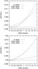 |
Fig. 7 Bias due to the centroid offset. The solid line is our estimate (400 sets of data) without centroid offset. The plus (cross) points are estimate for the centroid offset alone the major (minor) axis of the elliptical halo. The top (bottom) panel is for galaxy halo with ellipticity 0.3 (0.6). |
4. Conclusions and outlook
In this paper, we have studied galaxy-galaxy flexion with elliptical mass distributions. We
derived the ratio r of radial and tangential flexion and found that it is
independent of the radial mass profile of the lens, and of the source and lens redshift. The
flexion ratio depends solely on the ellipticity and orientation of the mass distribution. We
defined an estimator
for the ellipticity in terms of the flexion ratio, and tested its performance with simple
simulations. This estimator does not rely on knowing the orientation of the distribution,
i.e., assuming that it follows the orientation of the light; hence, it can be used to
statistically superpose several lenses and thereby obtain their average ellipticity. The
independence of this estimator from an assumed orientation is quite different from methods
to constrain lens ellipticities from shear (Brainerd
& Wright 2000; Hoekstra et al.
2004), for which the orientation needs to be known. In the appendix we show that an
analogous method to that presented here does not work for shear, but is unique to the spin-1
nature of the first flexion.
For an individual lens with several flexion measurements, the ellipticity and orientation
can be derived by fitting the measured flexion ratios with these two parameters. The
accuracy of the resulting estimate is substantially better than that of
.
Our simulations showed that
is biased. A first bias is due to the non-linearity of the relation between estimated
ellipticity and mean flexion ratio. The size of this bias depends on the number density of
sources for which flexion can be measured, and disappears in the limit of very high source
density (or large number of lenses for which the mean ellipticity is explored). Intrinsic
flexion causes a more significant bias, in particular for small values of
ϵ. A misidentification of the mass centroid is another source of bias;
however, if the centroid offset is much smaller than the Einstein radius of the lens, this
bias is rather small.
There will be several complications in a real analysis. First, the flexion ℱ can not be
directly measured, but only reduced flexion (Schneider
& Er 2008). This only requires a small modification, though: if
κ is constant on ellipses, so will be ln(1 − κ). Since
 (18)where
G1 is the spin-1 reduced flexion,
(18)where
G1 is the spin-1 reduced flexion,
 , and
g = γ/(1 − κ) the reduced shear, we
can use the phase of (18) instead of the
flexion ratio. Furthermore, the impact of intrinsic flexion is uncertain, reflecting our
lack of knowledge about its magnitude which is ill-determined from current observations. A
further careful study of intrinsic flexion will be of interest before the flexion method is
applied to real data.
, and
g = γ/(1 − κ) the reduced shear, we
can use the phase of (18) instead of the
flexion ratio. Furthermore, the impact of intrinsic flexion is uncertain, reflecting our
lack of knowledge about its magnitude which is ill-determined from current observations. A
further careful study of intrinsic flexion will be of interest before the flexion method is
applied to real data.
In addition, as we have shown, a low number density of background sources also introduce bias. Thus a deep survey with more background sources is clearly favoured. Current surveys such as the Hubble Space Telescope (HST), the Canada-France-Hawaii Telescope Legacy Survey (CFHTLS) or Subaru telescope might be able to constrain halo ellipticity using flexion, if the flexion can be measured with sufficient accuracy. The James Webb Space Telescope will almost certainly allow very accurate measurements of the ellipticity of galaxy- and group-sized lenses.
Acknowledgments
We thank Dave Goldberg, Ismael Tereno and the anonymous referee for very useful comments on the manuscript. This project is supported by the Deutsche Forschungsgemeinschaft under the project SCHN 342/7.
References
- Allgood, B., Flores, R. A., Primack, J. R., et al. 2006, MNRAS, 367, 1781 [NASA ADS] [CrossRef] [Google Scholar]
- Bacon, D. J., Goldberg, D. M., Rowe, B. T. P., & Taylor, A. N. 2006, MNRAS, 365, 414 [NASA ADS] [CrossRef] [Google Scholar]
- Bacon, D. J., Amara, A., & Read, J. I. 2010, MNRAS, 1249 [Google Scholar]
- Bartelmann, M., & Schneider, P. 2001, Phys. Rep., 340, 291 [NASA ADS] [CrossRef] [Google Scholar]
- Beers, T. C., Flynn, K., & Gebhardt, K. 1990, AJ, 100, 32 [NASA ADS] [CrossRef] [Google Scholar]
- Bett, P., Eke, V., Frenk, C. S., Jenkins, A., & Okamoto, T. 2010, MNRAS, 404, 1137 [NASA ADS] [Google Scholar]
- Bradač, M., Allen, S. W., Treu, T., et al. 2008, ApJ, 687, 959 [NASA ADS] [CrossRef] [Google Scholar]
- Brainerd, T. G., & Wright, C. O. 2000, unpublished [arXiv:astro-ph/0006281] [Google Scholar]
- Clowe, D., Bradač, M., Gonzalez, A. H., et al. 2006, ApJ, 648, L109 [NASA ADS] [CrossRef] [Google Scholar]
- Corless, V. L., King, L. J., & Clowe, D. 2009, MNRAS, 393, 1235 [NASA ADS] [CrossRef] [Google Scholar]
- Deb, S., Goldberg, D. M., Heymans, C., & Morandi, A. 2010, ApJ, 721, 124 [NASA ADS] [CrossRef] [Google Scholar]
- Debattista, V. P., Moore, B., Quinn, T., et al. 2008, ApJ, 681, 1076 [NASA ADS] [CrossRef] [Google Scholar]
- Er, X., Li, G., & Schneider, P. 2011, A&A, submitted [arXiv:1008.3088] [Google Scholar]
- Evans, A. K. D., & Bridle, S. 2009, ApJ, 695, 1446 [NASA ADS] [CrossRef] [EDP Sciences] [Google Scholar]
- Goldberg, D. M., & Bacon, D. J. 2005, ApJ, 619, 741 [NASA ADS] [CrossRef] [Google Scholar]
- Goldberg, D. M., & Leonard, A. 2007, ApJ, 660, 1003 [NASA ADS] [CrossRef] [Google Scholar]
- Goldberg, D. M., & Natarajan, P. 2002, ApJ, 564, 65 [NASA ADS] [CrossRef] [Google Scholar]
- Hawken, A. J., & Bridle, S. L. 2009, MNRAS, 400, 1132 [NASA ADS] [CrossRef] [Google Scholar]
- Hoekstra, H., Yee, H. K. C., & Gladders, M. D. 2004, ApJ, 606, 67 [NASA ADS] [CrossRef] [Google Scholar]
- Howell, P. J., & Brainerd, T. G. 2010, MNRAS, 941 [Google Scholar]
- Irwin, J., & Shmakova, M. 2006, ApJ, 645, 17 [NASA ADS] [CrossRef] [Google Scholar]
- Jing, Y. P., & Suto, Y. 2002, ApJ, 574, 538 [NASA ADS] [CrossRef] [Google Scholar]
- Kormann, R., Schneider, P., & Bartelmann, M. 1994, A&A, 284, 285 [NASA ADS] [Google Scholar]
- Kuhlen, M., Diemand, J., & Madau, P. 2007, ApJ, 671, 1135 [NASA ADS] [CrossRef] [Google Scholar]
- Law, D. R., Majewski, S. R., & Johnston, K. V. 2009, ApJ, 703, L67 [NASA ADS] [CrossRef] [Google Scholar]
- Leonard, A., Goldberg, D. M., Haaga, J. L., & Massey, R. 2007, ApJ, 666, 51 [NASA ADS] [CrossRef] [Google Scholar]
- Mandelbaum, R., Hirata, C. M., Broderick, T., Seljak, U., & Brinkmann, J. 2006, MNRAS, 370, 1008 [NASA ADS] [CrossRef] [Google Scholar]
- Massey, R., Rowe, B., Refregier, A., Bacon, D. J., & Bergé, J. 2007, MNRAS, 380, 229 [NASA ADS] [CrossRef] [Google Scholar]
- Munshi, D., Valageas, P., van Waerbeke, L., & Heavens, A. 2008, Phys. Rep., 462, 67 [NASA ADS] [CrossRef] [Google Scholar]
- Natarajan, P., & Refregier, A. 2000, ApJ, 538, L113 [NASA ADS] [CrossRef] [Google Scholar]
- Navarro, J. F., Frenk, C. S., & White, S. D. M. 1996, ApJ, 462, 563 [NASA ADS] [CrossRef] [Google Scholar]
- Navarro, J. F., Frenk, C. S., & White, S. D. M. 1997, ApJ, 490, 493 [NASA ADS] [CrossRef] [Google Scholar]
- Oguri, M., Takada, M., Okabe, N., & Smith, G. P. 2010, MNRAS, 405, 2215 [NASA ADS] [Google Scholar]
- Okura, Y., Umetsu, K., & Futamase, T. 2007, ApJ, 660, 995 [NASA ADS] [CrossRef] [Google Scholar]
- Okura, Y., Umetsu, K., & Futamase, T. 2008, ApJ, 680, 1 [NASA ADS] [CrossRef] [Google Scholar]
- Parker, L. C., Hoekstra, H., Hudson, M. J., van Waerbeke, L., & Mellier, Y. 2007, ApJ, 669, 21 [Google Scholar]
- Refregier, A. 2003, ARA&A, 41, 645 [NASA ADS] [CrossRef] [Google Scholar]
- Schneider, P., & Er, X. 2008, A&A, 485, 363 [NASA ADS] [CrossRef] [EDP Sciences] [Google Scholar]
- Schneider, P., Kochanek, C. S., & Wambsganss, J. 2006, Gravitational Lensing: Strong, Weak and Micro, ed. P. Schneider, C. S. Kochanek, & J. Wambsganss [Google Scholar]
- Suyu, S. H., & Halkola, A. 2010, A&A, 524, A94 [NASA ADS] [CrossRef] [EDP Sciences] [Google Scholar]
Appendix A: The shear profile in SIE halo
In this appendix, we present the tangential and cross shear profile for an SIE halo model and show that one cannot apply the ratio of cross to tangential shear to estimate the ellipticity of the lens.
To calculate the shear, we calculate the deflection potential using the Poisson equation
 (A.1)The convergence can
be written in polar coordinates
(A.1)The convergence can
be written in polar coordinates  (A.2)where f
is the axs ratio. The solution of the Poisson equation can be found in Kormann et al. (1994), but here we write it in our
notation as
(A.2)where f
is the axs ratio. The solution of the Poisson equation can be found in Kormann et al. (1994), but here we write it in our
notation as  (A.3)where
 .
Then we rewrite the potential in Cartesian coordinates and calculate the shear by
γ1 = (ψ,11 − ψ,22)/2
and γ1 = ψ,12. We thus obtain the
two shear component for the SIE halo,
.
Then we rewrite the potential in Cartesian coordinates and calculate the shear by
γ1 = (ψ,11 − ψ,22)/2
and γ1 = ψ,12. We thus obtain the
two shear component for the SIE halo, ![Mathematical equation: \appendix \setcounter{section}{1} \begin{eqnarray} \gamma_1 &=&-\dfrac{\theta_{\rm E} (1-\epsilon)(\theta_1^2-\theta_2^2)} {2\theta^2 d}; \\[5mm] \gamma_2 &=&-\dfrac{ \theta_{\rm E} (1-\epsilon) \theta_1\theta_2} {\theta^2 d}, \end{eqnarray}](/articles/aa/full_html/2011/04/aa15766-10/aa15766-10-eq96.png) where
where
 .
According to the definition
γt = −γ1cos2φ − γ2sin2φ,
γ × = γ1sin2φ − γ2cos2φ,
the tangential-to-cross shear for SIE halo reads
.
According to the definition
γt = −γ1cos2φ − γ2sin2φ,
γ × = γ1sin2φ − γ2cos2φ,
the tangential-to-cross shear for SIE halo reads ![Mathematical equation: \appendix \setcounter{section}{1} \begin{eqnarray} \gamma_{\rm t} &=& {\theta_{\rm E}(1-\epsilon) \over 2 d};\\[5mm] \gamma_{\times} &=& 0. \end{eqnarray}](/articles/aa/full_html/2011/04/aa15766-10/aa15766-10-eq100.png)
All Figures
|
Fig. 1 Spin-1 flexion vector field for an elliptical isothermal density distribution with ϵ = 0.3. ℱ only points towards the center when the background galaxy is located on the major or minor axis of the halo. Note that the length of the vectors are logarithmically scaled, for better visibility. |
| In the text | |
|
Fig. 2 Comparison of the ellipticity estimator (14) with the input ellipticity (solid line). The estimated ellipticity for 20 realizations each for 20 input values of ϵ are shown by pluses, for NIE models with θc = 2′′. |
| In the text | |
|
Fig. 3 Top panel: comparison of the input ellipticity (solid line) and the estimate (similar as Fig. 2). The plus points show the average estimate for 20 realizations without noise. The other are the result from data with intrinsic noise. All the result are calculated from Eq. (14). The stars are calculated when flexion ratios higher than the upper limit (Eq. (11)) are excluded. Bottom panel: fractional error |δϵ/ϵ| of our estimate for the respective cases. |
| In the text | |
|
Fig. 4 Histogram of the estimated ellipticity for a halo with ϵ = 0.57 from 20 realizations. The solid line is obtained from noise data, the dashed line is the result after excluding the high flexion ratio points. |
| In the text | |
|
Fig. 5 Comparison of mean estimator and biweight estimator. The plus point are the result using mean estimate The crosses are the result using biweight center estimate Eq. (15) to calculate ⟨ r ⟩ . |
| In the text | |
|
Fig. 6 The flexion ratio r varies with φ. The dashed line is for an SIE halo model. The points are calculated from the simulated data, the dotted line is the fit to the results with Eq. (9). Left is a halo with ϵ = 0.3, and right is ϵ = 0.6. |
| In the text | |
|
Fig. 7 Bias due to the centroid offset. The solid line is our estimate (400 sets of data) without centroid offset. The plus (cross) points are estimate for the centroid offset alone the major (minor) axis of the elliptical halo. The top (bottom) panel is for galaxy halo with ellipticity 0.3 (0.6). |
| In the text | |
Current usage metrics show cumulative count of Article Views (full-text article views including HTML views, PDF and ePub downloads, according to the available data) and Abstracts Views on Vision4Press platform.
Data correspond to usage on the plateform after 2015. The current usage metrics is available 48-96 hours after online publication and is updated daily on week days.
Initial download of the metrics may take a while.