| Issue |
A&A
Volume 528, April 2011
|
|
|---|---|---|
| Article Number | A124 | |
| Number of page(s) | 11 | |
| Section | Extragalactic astronomy | |
| DOI | https://doi.org/10.1051/0004-6361/201015739 | |
| Published online | 14 March 2011 | |
Galaxy evolution and star formation efficiency at 0.2 < z < 0.6⋆
1
Observatoire de Paris, LERMA
(CNRS:UMR8112), 61 Av. de l’Observatoire, 75014 Paris, France
e-mail: This email address is being protected from spambots. You need JavaScript enabled to view it.
2
Observatorio Astronómico Nacional
(OAN)-Observatorio de Madrid, Alfonso XII, 3, 28014- Madrid, Spain
3
Laboratoire d’Astrophysique de
Bordeaux, UMR 5804, Université Bordeaux I, BP 89, 33270
Floirac,
France
4
Max-Planck-Institut für Astronomie
(MPIA), Königstuhl
17, 69117
Heidelberg,
Germany
5
IEM, Consejo Superior de
Investigaciones Cientificas (CSIC), Serrano 121, 28006
Madrid,
Spain
Received: 10 September 2010
Accepted: 4 February 2011
Abstract
We present the results of a CO line survey of 30 galaxies at moderate redshift (z ~ 0.2−0.6), with the IRAM 30 m telescope, with the goal to follow galaxy evolution and in particular the star formation efficiency (SFE) as defined by the ratio between far-infrared luminosity and molecular gas mass (LFIR/M(H2)). The sources are selected to be ultra-luminous infra-red galaxies (ULIRGs), with LFIR larger than 2.8 × 10¹² L⊙, experiencing starbursts; adopting a low ULIRG CO-to-H2 conversion factor, their gas consumption time-scale is lower than 108 yr. To date only very few CO observations exist in this redshift range that spans nearly 25% of the universe’s age. Considerable evolution of the star formation rate is already observed during this period. 18 galaxies out of our sample of 30 are detected (of which 16 are new detections), corresponding to a detection rate of 60%. The average CO luminosity for the 18 galaxies detected is  K km s-1 pc2, corresponding to an average H2 mass of 1.6 × 10¹⁰ M⊙. The FIR luminosity correlates well with the CO luminosity, in agreement with the correlation found for low and high redshift ULIRGs. Although the conversion factor between CO luminosity and H2 mass is uncertain, we find that the maximum amount of gas available for a single galaxy is quickly increasing as a function of redshift. Using the same conversion factor, the SFEs for z ~ 0.2 − 0.6 ULIRGs are found to be significantly higher, by a factor 3, than for local ULIRGs, and are comparable to high redshift ones. We compare this evolution to the expected cosmic H2 abundance and the cosmic star formation history.
Key words: galaxies: high-redshift / galaxies: ISM / galaxies: starburst / radio lines: galaxies
Based on observations carried out with the IRAM 30 m telescope. IRAM is supported by INSU/CNRS (France), MPG (Germany) and IGN (Spain).
© ESO, 2011
1. Introduction
Ultra-luminous infra-red galaxies (ULIRGs) emit most of their energy in the far-infrared, and have far-infrared luminosities LFIR > 1012 L⊙, (e.g. Sanders & Mirabel 1996; Veilleux et al. 2009). Since they can be seen so far away, they allow us to explore the evolution of star formation in the universe, and of the star formation efficiency (SFE) in particular, defined as the FIR luminosity to H2 mass ratio (e.g. Kennicutt 1998). Since the discovery of the first high redshift object in CO line emission (IRAS F10214+4724 at z = 2.3, Brown & Vanden Bout 1991; Solomon et al. 1992), there has been a wealth of CO-line discoveries, a hundred objects are now detected at z > 1, either from ULIRGs, or from LIRGs (LFIR > 1011 L⊙). Some are amplified by gravitational lensing (see the review by Solomon & Vanden Bout 2005). They allow us to observe the interstellar medium of the galaxies, the CO excitation (e.g. Weiss et al. 2007) and estimate the amount of molecular gas present. Stars form from molecular gas, so it is important to infer the H2 mass in order to determine the SFE. At high redshift, many of these objects are quasars or radio-galaxies (due to their selection, e.g. Omont et al. 2003), however, their FIR emission is powered predominantly by star formation (e.g. Riechers et al. 2009; Wang et al. 2010).
Locally, our knowledge of the ULIRG phenomenon is more profound due to higher spatial resolution and sensitivity. Because the peak of the dust emission is progressively shifted from the FIR to the submm domain, the dust emission can be detected to high redshifts (negative K-correction, e.g. Blain & Longair 1996). The CO-line emission is less favoured, and CO lines are difficult to detect at high z although observing the high-J CO lines helps significantly in highly excited objects (Combes et al. 1999). To date, more than a hundred objects have been studied in detail locally. In the case of the ULIRGs, it was found that they are characterized by compact, nuclear starbursts (e.g. Downes & Solomon 1998), and it has been argued that a special CO-to-H2 conversion factor should be used, that is 5.75 lower than the standard factor commonly used for Milky Way-like galaxies (Downes et al. 1993). In the present paper, we will adopt for ULIRGs the ratio α = 0.8 (Solomon et al. 1997) between M(H2) and  , expressed in units of M⊙ (K km s-1 pc2)-1, and not the standard α = 4.6.
At intermediate redshifts, between 0.2 < z < 1, there is a dearth of CO-line detections. This is partly due to observational difficulties. The most commonly used millimetric window is the 3 mm one, which is least affected by atmospheric opacity. Between 81 and 115 GHz, all redshifts can be observed with at least one line of the CO rotational ladder, except between z = 0.4 and 1. The latter can be observed at 2 mm (targeting the CO(2 − 1) line), but in less favorable atmospheric conditions. While between z = 0.2 and z = 0.4 the 3 mm window can be used in the CO(1 − 0) transition, the K-correction is strongly reducing its observable intensity (by a factor growing faster than (1 + z)4, Combes et al. 1999). The redshift range 0.2 < z < 1 is important though, as it covers almost half of the age of the universe, and also the most dramatic change in star formation activity (e.g. Madau et al. 1998; Hopkins & Beacom 2006). In the universal star formation history, the most striking feature is the impressive drop between z = 1 and z = 0 by at least an order of magnitude (Blain et al. 1999).
Up to now, very little was known about the molecular gas content of galaxies at moderate redshift. The ULIRG sample of Solomon et al. (1997) contains 37 objects, but only 2 have z > 0.2. Negative results were obtained in previous studies, conducted about 10 yrs ago (Lo et al. 1999; Wilson & Combes 1998), but the performances of the mm-instruments have dramatically improved since then. Two more objects were detected by Geach et al. (2009), although more upper limits were also reported (Melchior & Combes 2008). To study star forming galaxies in this period, and in particular to derive their star formation efficiency, we have undertaken a CO-line search in the range 0.2 < z < 0.6, almost unknown territory as far as molecular lines are concerned. We have selected a sample of 30 IR-luminous galaxies in this redshift range to check whether the variation of star forming activity is due to a variation in molecular gas content or star formation efficiency, or both. One of the objects (IRAS 11582+3020, hereafter G4) has already been mapped with the IRAM Plateau de Bure Interferometer (Combes et al. 2006, Paper I). The CO map showed spatially resolved emission on 30 kpc scales and revealed a velocity gradient. It was concluded in that paper that not all the molecular gas is confined in a nuclear starburst, but that ~ 50% of it is extended on galactic scales (25 − 30 kpc). In the present paper, we describe the CO survey carried out with the IRAM 30 m telescope. The sample is described in Sect. 2 and the observations in Sect. 3. Results are presented in Sect. 4 and discussed in Sect. 5.
2. The sample
The present-day sensitivity in the CO line restricted the sample to the brightest objects in the far infrared. We have selected all objects between 0.2 < z < 0.6 and Dec(2000) > −12° that are identified as galaxies in the literature, have spectroscopic redshifts, and are detected at 60 μm (IRAS, ISO). This resulted in a total of 209 galaxies. Most of the galaxies (and in particular the brightest ones) have detailed photometry in the NIR bands, from the samples by Clements et al. (1996), Kim & Sanders (1998), Kim et al. (2002) and Stanford et al. (2000). The available sub-arcsec K-band images (from either IRTF or Keck telescopes, in the above references), reveal that about two-thirds of the objects are interacting galaxies.
Out of the 209 galaxy sample, we selected the brightest ones, with log LFIR > 12.45. This leads to a sample of 36 objects, to be observed with the 30 m telescope. We did not reobserve one galaxy detected by Solomon et al. (1997), nor 3C48, detected by Wink et al. (1997), although we include these 2 sources in our analysis. Due to weather conditions, only 28 sources were observed in the project. All their identification and coordinates are displayed in Table 1. Out of the 30 objects in the sample (including the two literature sources), 18 were detected, corresponding to a detection rate of 60%. Figure 1 displays the distribution of FIR luminosities with redshift.
 |
Fig. 1 Definition of our sample. Among the 209 northern galaxies (filled symbols) found in NED between 0.2 < z < 0.6 and detected at 60 μm by IRAS, we selected the most luminous ones (log LFIR/L⊙ > 12.45, as indicated by the horizontal line). By comparison, the ULIRGs in the sample of Solomon et al. (1997) are plotted as open triangles. The circles indicate detections, non-detections are marked by a cross. Sources that have neither a circle nor a cross could not be observed due to weather conditions. |
Definition of the sample.
Observed line parameters.
The far-infrared fluxes FFIR are computed as 1.26 × 10⁻¹⁴ (2.58 S60 + S100) W m-2 (Sanders & Mirabel 1996). The far-infrared luminosity is then  CC FFIR, where DL is the luminosity distance, and CC the color correction, CC = 1.42 (e.g. Sanders & Mirabel 1996). The FIR-to-radio ratio q = log ([FFIR/(3.75 × 1012 Hz)]/[fν(1.4 GHz)]) has been computed for sources where radio data were available; the radio fluxes are listed in Table 2. Excluding the radio galaxies 3C48 and 3C345, the average is q = 2.3, typical for ULIRGs (Sanders & Mirabel 1996). The star formation rates of all sample galaxies are above 480 M⊙ yr-1, estimated from the infrared luminosity (e.g. Kennicutt 1998).
In this article, we adopt a standard flat cosmological model, with Λ = 0.73, and a Hubble constant of 71 km s-1 Mpc-1 (Hinshaw et al. 2009).
 |
Fig. 2 The CO spectra of the detected galaxies. The zero velocity scale corresponds to the optically determined redshift, listed in Table 1. Sources detected in CO(3–2) at 1mm wavelength are also shown. Some sources were detected in CO(1–0) but not in CO(3–2), as indicated in Table 2. The vertical scale is Tmb in mK. The spectrum of G4 is already presented in Paper I. |
3. Observations
The observations were carried out with the IRAM 30 m telescope at Pico Veleta, Spain, between January 2005 and January 2006. Most of the galaxies, with redshifts between 0.2 and 0.39, could be observed simultaneously at 3 mm in CO(1 − 0) and at 1 mm in CO(3 − 2), except the two lowest redshift sources (G4 and G5) where only observations in the 3 mm band were possible. In any case, the weather prevented us sometimes from taking useful data at 1 mm. For the highest redshift sources (G19, G20, G23, G27 and G28), only the CO(2 − 1) line was observed in the 2 mm band.
The SIS receivers were tuned in single sideband mode to the redshifted frequencies of the various CO lines. The observations were carried out in wobbler switching mode, with reference positions offset by 3′ in azimuth. We used the 1 MHz back-ends with an effective total bandwidth of 512 MHz at 3 mm (providing a ~ 1500 km s-1 range) and the 4 MHz filterbanks with an effective total bandwidth of 1024 MHz at 1 mm.
We spent 2–4 h on each galaxy, resulting in a relatively homogeneous noise level of 1–2 mK per 30 km s-1 channel for all sources. The system temperatures ranged between 120 and 250 K at 3 mm, between 220 and 300 K at 2 mm, and between 300 and 500 K at 1.2 mm, in  . The pointing was regularly checked on continuum sources and yielded an accuracy of 3′′ rms. The temperature scale used is in main beam temperature Tmb. At 3 mm, 2 mm and 1 mm, the telescope half-power beam width is 27′′, 17′′ and 10′′ respectively. The main-beam efficiencies are η
 , 0.70 and 0.64, respectively, and S/Tmb = 4.8 Jy/K for all bands.
Each spectrum was summed and reduced using linear baselines, and then binned to 50 − 60 km s-1 channels for the plots.
4. Results
4.1. CO detection in z = 0.2 − 0.6 ULIRGs
All spectra for CO detections are displayed in Figs. 2–4 (except G4 reported in Paper I). The non-detections are reported in Table 2. Integrated upper limits are computed at 3σ, assuming a common line-width of 300 km s-1, and getting the rms of the signal over 300 km s-1. Lines are assumed detected when the integrated signal is larger than 3σ. Gaussian fits then yielded the central velocities, velocity FWHMs and integrated fluxes listed in Table 2.
As already noticed in Sect. 2, very few objects were previously detected in CO in this redshift range. We include in our analysis, and in Table 2, two additional ULIRGs (G29 and G30) that satisfy our sample criteria. In the discussion, we also added the two galaxies on the outskirts of the cluster Cl 0024+16 (Geach et al. 2009); they are not ULIRGs, but it is interesting to compare star formation efficiencies for all CO-detected objects in this redshift range.
The detection rate of 60% in our sample, down to a sensitivity limit of ~1.5 Jy km s-1, must be considered a lower limit. Indeed, the available velocity range of the receivers (about 1500 km s-1) could have missed some sources if the optical redshift was not accurate enough. Some galaxies show a significant velocity offset (e.g. G17) as can be seen in Table 2 and the figures. Some of the profiles may have a double-horn shape as G18, but most do not, given our spectral resolution and sensitivity. The line-widths detected are compatible with massive galaxies at random inclinations. Their average is ΔVFWHM = 348 km s-1, very similar to the value for local ULIRGs of 302 km s-1 (Solomon et al. 1997). In comparison, the submillimeter galaxies have much broader widths, 655 km s-1 on average (Greve 2005). Given the angular distance of the sources (average value 1000 Mpc), our beam subtends between 50 and 100 kpc, and all galaxies can be considered unresolved, at least as far as their molecular component is concerned.
4.2. CO luminosity and H2 mass
To derive the total H2 mass, we first compute the CO luminosity through integrating the CO intensity over the velocity profile.
The CO luminosity for a high-z source is given by
 where ICO is the intensity in K km s-1, ΩB is the area of the main beam in square arcseconds and DL is the luminosity distance in Mpc. We assume here that the sources are unresolved, in our beam of typically 50 − 100 kpc. We then compute H2 masses using
  , with α = 0.8 M⊙ (K km s-1 pc2)-1, for ULIRGs. The molecular gas masses are listed in Table 3. Although it could be advocated that a different conversion factor should apply to some of the galaxies, we always refer to the M(H2) mass, directly proportional to CO luminosity, for the sake of comparison. For those galaxies where we observed two CO transitions, we used the CO luminosity of the lower transition to calculate H2 masses. In our sample, most galaxies have CO(1 − 0) data, except three galaxies, G19, G23 and G27, which have been detected in CO(2 − 1). We assume that the brightness temperatures are similar in the two lines, as expected for an optically thick, and thermally excited medium. The problem is more severe for high-z objects, where the CO excitation is not well-known. The average CO luminosity for the 18 galaxies detected is
  K km s-1 pc2, corresponding to an average H2 mass of 1.6 × 10¹⁰ M⊙.
The star formation efficiency (SFE), also listed in Table 3, is defined as LFIR/M(H2) in L⊙/M⊙. Since the SFR is related to the FIR luminosity as SFR = LFIR /(5.8 × 109L⊙) (e.g. Kennicutt 1998), the gas consumption time-scale can be derived by τ = 5.8/SFE Gyr.
Molecular gas mass and star formation efficiency.
CO gas excitation.
4.3. Molecular gas excitation
Three sources have been detected in both the CO(1−0) and CO(3−2) lines, and three have upper limits, as listed in Table 4. For the data points, we took the peak flux Sν of the lines, since the CO(3−2) and CO(1−0) have sometimes different measured linewidths, which could be due partly to the noise. The corresponding ratio between the peak brightness temperatures are also displayed in Table 4, to compare more easily with the predictions of the model.
 |
Fig. 5 Peak Tb ratio between the CO(3−2) and CO(1−0) lines versus the H2 density, and the CO column density per unit velocity width (NCO/ΔV) for two values of the kinetic temperature: Tk = 45 K, the dust temperature (left), and Tk = 20 K (right). The black contours are underlining the values obtained in the data. The predictions come from the LVG hypothesis in the Radex code. |
The peak flux ratio between the two lines S32/S10, and equivalently the peak brightness temperature ratio, is a good indicator of the average density of the emitting medium, since density is the main factor determining the excitation. Another factor is the kinetic temperature, which could be linked to the dust temperature (e.g. Weiss et al. 2003). In Table 3, we have computed the dust temperature deduced from the far-infrared fluxes, assuming κν ∝ νβ, where κν is the mass opacity of the dust at frequency ν, and β = 1.5. The average dust temperature for our sample is 46 ± 5 K. This is comparable to recent results for starburst galaxies, which have dust temperatures ≈ 40 K (e.g. Sanders & Mirabel 1996; Elbaz et al. 2010).
If the gas is predominantly heated by collisions with the dust, the gas temperature is expected to be lower than the dust temperature, at low density (e.g. Spitzer 1978). Alternatively, if the gas is heated directly from UV photons near star forming regions, or by shocks due to turbulence or perturbed dynamics, then the gas could be at much higher kinetic temperatures. Since we observe very low excitation temperatures, we consider it unlikely that, in average over the beam, the hot molecular gas is dominating the emission. We then assume a gas kinetic temperature lower than the dust temperature, in the following modeling.
Using the Radex code (van der Tak et al. 2007), we have computed the predicted main beam temperature ratio between the CO(3−2) and CO(1−0) lines, for several kinetic temperatures and as a function of H2 densities and CO column densities. Figure 5 shows these predictions for Tk = 45 and 20 K. The black contours delineate the range of observed values. In Table 4 we list the derived values for the n(H2) densities, for two values of the kinetic temperatures (45 and 20 K), and for a fixed column density per velocity width.
We adopted a column density of N(CO)/ΔV of 7 × 1016 cm-2/(km s-1), which assumes that all CO lines are optically thick. This number is at the right order of magnitude given the high molecular gas masses derived in Table 2. For M(H2) = 3 × 10¹⁰ M⊙, a typical CO abundance of CO/H2 = 10-4, and a linewidth of 300 km s-1, this column density corresponds to a homogenous disk of 3 kpc in size. Either the emitting CO gas is more concentrated, as in nuclear starbursts, i.e. the CO column density would be higher, or the gas extent is larger than 3 kpc, in which case we would have to take the clumping factor into acount. In any case, it is likely that the CO lines are optically thick.
The excitation of the CO gas appears quite low, implying a low average H2 density in our galaxies. Comparing to the different excitation patterns observed in other high-z starburst galaxies (Weiss et al. 2007), our galaxies are among the lowest excitation, comparable to the Milky Way or even lower.
For the estimations, we have assumed that our sources are unresolved. Increasing the size of the molecular disks, here supposed to be point like (wrt to the beam sizes) to for example > 6′′ would increase the Tb ratios by > 50%, and this would raise the required densities by, at most, a similar factor according to Fig. 5.
It should be kept in mind that error bars are large on the observed ratios. The average ratio is lower than 1.8 ± 0.6, taking into account the upper limits. However the conclusion of a rather low average H2 density is rather robust with respect to the error bars, since the predicted flux ratio is increasing very quickly with density in the model. We note that even with the extreme hypothesis of optically thin gas, the observations are only compatible with n(H2) < 3 × 103 cm-3, since the predicted ratio increases even more with density than in the thick case. It is also possible that some of the gas has a kinetic temperature much higher than the dust temperature, but then the derived H2 density is even lower.
 |
Fig. 6 Measured CO luminosities, corrected for amplification when known, but not for gas excitation, as a function of redshift. We compare our points (full black circles, and arrows as upper limits) with a compilation of high-z molecular gas surveys, and local ones: green triangles are from Gao & Solomon (2004), blue squares from Solomon et al. (1997), open circles from Chung et al. (2009), blue diamonds from Geach et al. (2009), black crosses from Iono et al. (2009), red stars, from Greve et al. (2005), green full circles from Daddi et al. (2010), blue asterisks from Genzel et al. (2010), and blue full circles from Solomon & vanden Bout (2005). For illustration purposes only, the red curve is the power law for ΩH2/ΩHI proposed by Obreschkow & Rawlings (2009). |
4.4. Variation with redshift
Does the molecular gas content of galaxies evolve with redshift? It is interesting to compare the CO luminosity of our sample with the wealth of data reported in the literature. Figure 6 shows all CO measurements as a function of redshift. This figure reveals that indeed our sample (full black circles) is filling in the CO redshift desert, although not completely. The rise of the CO luminosity that is observed at high redshift (z > 1) in fact begins as soon as z = 0.2−0.3.
This variation is meaningful in the sense that only the brightest objects have been selected here. Most of the variation with z comes from the fact that there are no extremely luminous objects at z < 0.2. In itself, it is already an interesting evolution, that has been discussed in previous works at high redshift (i.e. Solomon & vanden Bout 2005; Tacconi et al. 2010). The present work extends this variation in the intermediate redshift range, and suggests that the increase in gas content with z might begin as soon as z = 0.3. The possibility of undiscovered large CO luminosity objects locally is not high, given the good correlation between CO and FIR luminosity. These objects should have been discovered as ULIRGs.
To interpret this evolution, caveats have to be kept in mind. At high redshift, at least for some of the sources, the CO luminosity could be over-estimated by poorly known amplification factors due to lensing. The luminosities have been corrected for amplification, when known, but these uncertainties contribute to the large scatter. This is not the case for the sample from Daddi et al. (2010, green circles) or the sample from Genzel et al. (2010, blue asterisks). Another uncertainty comes from the CO gas excitation. The CO luminosities of high redshift ULIRGs come from the measured high-J lines, and the low-J lines are often not known. They could underestimate the H2 mass, since the subthermal excitation is likely to reduce their luminosity with respect to the local objects, observed in CO(1−0). We think, however, that the steep rise at 0.2 < z < 0.6 of the most luminous galaxies discussed in this paper does not suffer from these caveats (they are detected in majority in CO(1 − 0) and are not lensed). It is interesting to note that the trend seen in Fig. 6 is essentially dominated by three galaxies, G1, G15 and G18, which are particularly strong in CO-emission. No such extreme has been found in the local universe. Two of these galaxies (G1 and G18) have been shown in Sect. 4.3 to be subthermally excited, and are likely extended starbursts with relatively low efficiency, as presented by Daddi et al. (2008). In Paper I, we also derived an extended gas disk for G4 with the Plateau de Bure observations. Table 3 confirms that G1 and G18 have among the lowest SFE of the sample. It is conceivable that the conversion factor between and M(H2) could be higher in these sources, leading to higher gas mass.
4.5. Correlation between FIR and CO luminosities
Figure 7 shows the well studied correlation between FIR and CO luminosities (e.g. Young & Scoville 1991). The correlation is non-linear, with the ultra-luminous objects displaying a higher FIR luminosity (i.e. star formation) for the amount of gas present, as implied by the lines plotted in the figure. Our sample galaxies fit perfectly in this picture, being all above the curve LFIR/M(H2) = 100 L⊙/M⊙ (corresponding to a consumption time-scale of τ = 58 Myr). One of the two galaxies detected above LFIR/M(H2) = 1000 L⊙/M⊙ (G19) has indications of nuclear activity (see Type in Table 3), but the second (G27) has none. We note that they are two of the three galaxies detected in CO(2−1), and not in CO(1−0); we have derived their H2 masses with the assumption of equal CO luminosity between these two first lines. If their gas was sub-thermally excited, their H2 mass could then be slightly under-estimated.
 |
Fig. 7 Correlation between FIR and CO luminosities, for our sample (full black circles, and arrows for upper limits) and the other points from the literature (same symbols as in Fig. 6). The 3 lines are for LFIR/M(H2) = 10, 100 and 1000 L⊙/M⊙ from bottom to top, assuming a conversion factor α = 0.8 M⊙ (K km s-1 pc2)-1. The three lines correspond to gas depletion time-scales of 580, 58 and 5.8 Myr respectively. |
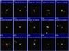 |
Fig. 8 Optical color images from the Sloan Digital Sky Survey (SDSS, http://www.sdss.org/) of 15 of our sources. They are all detections, except G10 and G21. Each panel is 50′′ × 50′′ in size, and is centered on the galaxy coordinates of Table 1. |
Assuming a dust temperature Td and the observed 100 μm flux S100, we can derive the dust mass as  where Sνo is the observed FIR flux measured in Jy,
  is the luminosity distance in Mpc, Bνr is the Planck function at the rest frequency νr = νo(1 + z), and we use a mass opacity coefficient of 25 cm2 g-1 at rest-frame 100 μm (Hildebrand 1983; Dunne et al. 2000; Draine 2003), with a frequency dependence of β = 1.5. Estimated dust masses are displayed in Table 3. If we adopt the low conversion factor of α = 0.8 M⊙ (K km s-1 pc2)-1, the average gas-to-dust mass ratio is 96 for all the detected galaxies. The gas to dust mass ratio could increase to up to 550 if the standard (MW) conversion factor is used. For local ULIRGs, this number is around 100 (Solomon et al. 1997), and 700 for normal galaxies (Wiklind et al. 1995), when calculated from IRAS fluxes.
We should note that the dust temperature has been measured from 60 and 100 μm fluxes, which correspond to (1 + z) higher frequencies in the rest frame of the galaxies. Therefore we are not sensitive to the very cold dust (~ 10 K).
4.6. Activity of the galaxies
We have made a census of the different activities occuring in our sample galaxies. The last column of Table 3 indicates nuclear AGN activity and/or perturbed morphology. These have been derived from the SDSS images, some of which are shown in Fig. 8. We note that among the 12 non-detections, there are only 4 active objects, all being Seyfert 1 or quasars, while among the 18 detected ones, there are 12 active objects, and most of the time they are LINERs, Seyfert 2, and show signs of galaxy interactions and mergers.
4.7. Star formation efficiency
In the following we adopt the definition of SFE = LFIR/M(H2), with a constant CO-to-H2 conversion factor. The average SFE in our sample is 555 L⊙/M⊙, 3 times higher than that of the local ULIRGs (170 L⊙/M⊙). It should be kept in mind that some galaxies could have a different conversion factor, and this uncertainty affects our conclusions. Also, it is possible that the local SFR tracers evolve with time, and that, for a given SFR, different amounts of gas are consumed in star formation, if the IMF (Initial Mass Function) is different for earlier and younger galaxies. However, no strong evidence has been found until now for a significantly changing IMF, and the star formation laws are remarkably constant over redshift, as discussed by Genzel et al. (2010) and Daddi et al. (2010). We plot the SFE versus in Fig. 9, versus LFIR in Fig. 11, and versus the dust temperature in Fig. 12.
 |
Fig. 9 Star formation efficiency SFE = LFIR/M(H2), versus CO luminosity, assuming the same CO-to-H2 conversion factor α = 0.8 M⊙ (K km s-1 pc2)-1. All symbols are as defined in Fig. 6. |
What is obvious in all these figures is that galaxies of our sample are among the most efficient forming stars, and G19 and G27 even lie above the starbursts at high redshift. They are not among the most gas-rich, according to the CO luminosity. They could be experiencing a burst due to galaxy interactions. This is the case for G19 (Fig. 8). No image is available for G27 (which lies outside of the footprint of the SDSS). Note that, as expected, there is a much larger correlation between SFE and LFIR, than with . The presence of large amounts of gas is not a sufficient condition to trigger a starburst, and another hidden factor is the extent of the spatial distribution of the molecular gas.
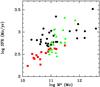 |
Fig. 10 The star formation rate (SFR) obtained from the far infrared luminosity, versus the stellar mass of galaxies in our sample (full black circles), compared to the sample of Da Cunha et al. (2010, full red squares) and Fiolet et al. (2009, full green triangles). |
To estimate the relative gas fractions of our sample galaxies, an estimation of their stellar and/or dynamical mass is required. We have tried to estimate the stellar mass from optical and near-infrared luminosities, taken from the literature, mainly the SDSS and 2MASS catalogs. The multi-wavelength luminosities were K-corrected according to the colors (e.g. Chilingarian et al. 2010), and stellar masses estimated according also to the colors (Bell et al. 2003). Stellar masses were found between 1010 and 1012 M⊙ or somewhat higher in the case of quasars. Figure 10 displays the star formation rate, derived from the infrared luminosity, versus the stellar mass, in comparison to the ULIRG samples of Da Cunha et al. (2010) and Fiolet et al. (2009). Our sample points follow the general trend, with the bias of strong SFR, due to our selection on L(FIR). The gas fractions derived from these stellar masses show large variations, with 3 objects around 1%, but most of them are between 10% and 65%. Another estimation is the dynamical mass, derived from the observed CO linewidths. This can only be a rough estimate, since neither the inclinations of the galaxies, nor the extent of their CO emission, are known. Adopting a typical radius of 3 kpc, the dynamical masses are in the range of 1011 M⊙, and the derived gas fraction are in general a few percent, with a large scatter, up to 60%. Note that the derived stellar masses are on average larger than the dynamical masses; this is due to the radius we have selected (3 kpc) to estimate the dynamical masses. For the same velocity width, the dynamical mass scales as the radius. Firm conclusions cannot be drawn until CO maps are available. Indeed, it is possible that the sample has a wide range of radial extents and, consequently, conversion factors.
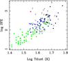 |
Fig. 12 Same as Fig. 9, but versus Td, for the sources where it could be defined. For the submillimeter galaxies, the red star corresponds to the averaged SFE, with the mean dust temperature of 35.5 found by Kovacs et al. (2010). |
Finally, there is a correlation between the dust temperature and the SFE in Fig. 12: it is conceivable that a concentrated starburst heats more efficiently the dust around it. However, the correlation becomes more scattered at higher redshifts, where the largest efficiencies occur. It is possible that our estimation of the dust temperature is not as accurate for these more redshifted objects. It is interesting to note the evolution of SFE with redshift, where our two most efficient starbursts are clearly noticeable, as shown in Fig. 13. We qualitatively compare this evolution with the cosmic star formation history, as compiled by Hopkins & Beacom (2006), from different works in the literature, and complemented at very high redshift by the gamma-ray burst (GRB) data of Kistler et al. (2009) and the optical data (Lyman-Break Galaxies, LBG) from Bouwens et al. (2008). The SFE logarithmic variations should be a combination between variations of the SFR and of the gas fraction in galaxies. It is interesting to superpose the observed logarithmic curve of these SFR variations to have an indication of the relative role of the various parameters. The schematic curve in log reproduces the relative variations, whatever the vertical units, and can be arbitrarily translated vertically. Our points correspond to the most drastic change in this curve, and our following study at 0.6 < z < 1 should give more insight in this epoch.
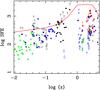 |
Fig. 13 Same as Fig. 9, but versus redshift. The red curve is a schematic line summarizing the cosmic star formation history, from the compilation by Hopkins & Beacom (2006), complemented with the GRB data by Kistler et al. (2009) and the optical data from Bouwens et al. (2008). The red curve is logarithmic and only indicative of relative variations of the star formation rate per cubic Mpc as a function of redshift, and can be translated vertically. |
5. Discussion and conclusions
We have presented our search for CO-line emission in a sample of 30 ULIRGs, selected between 0.2 < z < 0.6 to fill the gap or “CO redshift desert” between z = 0.1 and 1. We intend to cover the second part 0.6 < z < 1.0 in a following work. Our detection rate is ~60%. We find that some of the galaxies possess large amounts of molecular gas, much larger than local ULIRGs. Considering the evolution with cosmic time, it appears that the huge amounts of gas, common at high redshift, begin to disappear at z ~ 0.3. This drop in gas content is reminiscent of the drop in the star formation history of the universe, which may imply that the change in star formation is due to a change in gas content. There are good reasons to think that galaxies are more gas rich at high redshift, and also that their gaseous medium is denser. The sizes of galaxies are predicted to vary as (1 + z)-1, and the implied higher gas pressure could increase the H2/H I ratio. Following semi-analytical simulations, Obreschkow et al. (2009) followed the H2/H I ratio statistically over 30 million galaxies, and its cosmic decline has been modelled as ΩH2/ΩHI ∝ (1 + z)1.6 by Obreschkow & Rawlings (2009). This law appears to reproduce grossly the decline in the maximum with time, as shown in Fig. 6. Some galaxies of our sample, however, lie significantly above this envelope. The increase with z in the H2 content of galaxies might occur already at lower z than this model predicts.
Five of our galaxies were observed in both CO(3−2) and CO(1−0) lines, allowing an estimation of the excitation temperature. They appear all very low, similar to what is observed in the Milky Way, or more normal galaxies, but also some local ULIRGs (Radford et al. 1991). These ULIRGs could be similar to those discovered by Daddi et al. (2008) at redshift z ~ 1.5. If a galactic conversion factor was adopted for these galaxies, as suggested by Daddi et al. (2010), their H2 mass would be even higher, and they would stand out even more in the cosmic H2 abundance.
We emphasize that the choice of the conversion factor is crucial for the interpretation of the results. We have adopted the ULIRG value proposed by Solomon et al. (1997), and derive large SFE and short consumption time-scales for the gas. These SFE values would be lower if a higher, i.e. the Galactic, conversion factor is used. However, for consistency with previous studies we prefer to assume only a single value for the conversion factor. The latter could vary with the extent of the molecular component. We do not yet have spatial information on the CO emission and future interferometer observations are required to constrain the conversion factor further.
We have compared the star formation history and the redshift evolution of the SFE. It is expected that the latter evolves as a combination of the SFR and gas fraction evolution. It is likely that the star formation decline between z = 1 and z = 0 is partly due to the declining star forming efficiency. For galaxies of our sample, the star formation efficiency (SFE) appears very high, in comparison to the most active starbursts at different redshifts. This supports a high contribution of the SFE to the star formation variations with redshift, although we are observing an increase of efficiency of the most extreme objects. It is possible to compare the observed time gradients in the cosmic star formation rate, and those in the extreme SFE in Fig. 13. We observe a significant gradient in SFE, but however less steep than in the star formation history. The latter requires also a strong variation in gas content.
The very efficient star forming objects (ULIRGs) dominate the star formation at high redshift (z < 1.5, Lefloc’h et al. 2005), and less extreme objects (LIRGs) dominate later on (Caputi et al. 2006), which might explain the strong decline in efficiency between z = 1 and 0. It appears that the range of redshift studied here is just where the most massive objects continue to form stars with unprecedented efficiency, before the sudden drop due to star formation quenching (e.g. Springel et al. 2005).
Acknowledgments
We warmly thank the referee for his/her constructive comments and suggestions. The IRAM staff is gratefully acknowledged for their help in the data acquisition. We have made use of the NASA/IPAC Extragalactic Database (NED).
References
- Bell, E., McIntosh, D. H., Katz, N., & Weinberg, M. D. 2003, ApJS, 149, 289 [NASA ADS] [CrossRef] [Google Scholar]
- Blain, A. W., & Longair, M. S. 1996, MNRAS, 279, 847 [NASA ADS] [Google Scholar]
- Blain, A. W., Smail, I., Ivison, R. J., & Kneib, J.-P. 1999, MNRAS, 302, 632 [NASA ADS] [CrossRef] [Google Scholar]
- Bouwens, R. J., Illingworth, G. D., Franx, M., & Ford, H. 2008, ApJ, 686, 230 [NASA ADS] [CrossRef] [Google Scholar]
- Brown, R. L., & Van den Bout, P. A. 1991, AJ, 102, 1956 [NASA ADS] [CrossRef] [Google Scholar]
- Caputi, K. I., Dole, H., Lagache, G., et al. 2006, A&A, 454, 143 [NASA ADS] [CrossRef] [EDP Sciences] [Google Scholar]
- Chilingarian, I. V., Melchior, A.-L., & Zolotukhin, I. 2010, MNRAS, 405, 1409 [NASA ADS] [CrossRef] [Google Scholar]
- Chung, A., Narayanan, G., Yun, M. S., Heyer, M., & Erickson, N. R. 2009, AJ, 138, 858 [NASA ADS] [CrossRef] [Google Scholar]
- Clements, D., Sutherland, W., Saunders, W., et al. 1996, MNRAS, 279, 459 [NASA ADS] [CrossRef] [Google Scholar]
- Combes, F., Maoli, R., & Omont, A. 1999, A&A, 345, 369 [NASA ADS] [Google Scholar]
- Combes, F., García-Burillo, S., Braine, J., et al. 2006, A&A, 460, L49 (Paper I) [NASA ADS] [CrossRef] [EDP Sciences] [Google Scholar]
- Da Cunha, E., Charmandaris, V., Daz-Santos, T., et al. 2010, A&A, 523, A78 [NASA ADS] [CrossRef] [EDP Sciences] [Google Scholar]
- Daddi, E., Dannerbauer, H., Elbaz, D., et al. 2008, ApJ, 673, L21 [NASA ADS] [CrossRef] [Google Scholar]
- Daddi, E., Bournaud, F., Walter, F., et al. 2010, ApJ, 713, 686 [NASA ADS] [CrossRef] [Google Scholar]
- Downes, D., & Solomon, P. 1998, ApJ, 507, 615 [NASA ADS] [CrossRef] [Google Scholar]
- Downes, D., Solomon, P., & Radford, S. J. E. 1993, ApJ, 414, L13 [NASA ADS] [CrossRef] [Google Scholar]
- Draine, B. T. 2003, ARA&A, 41, 241 [NASA ADS] [CrossRef] [Google Scholar]
- Dunne, L., Eales, S., Edmunds, M., et al. 2000, MNRAS, 315, 115 [NASA ADS] [CrossRef] [Google Scholar]
- Elbaz, D., Hwang, H. S., Magnelli, B., et al. 2010, A&A, 518, L29 [NASA ADS] [CrossRef] [EDP Sciences] [Google Scholar]
- Fiolet, N., Omont, A., Polletta, M., et al. 2009, A&A, 508, 117 [NASA ADS] [CrossRef] [EDP Sciences] [Google Scholar]
- Gao, Y., & Solomon, P. M. 2004, ApJS, 152, 63 [NASA ADS] [CrossRef] [Google Scholar]
- Geach, J. E., Smail, I., Coppin, K., et al. 2009, MNRAS, 395, L62 [NASA ADS] [Google Scholar]
- Genzel, R., Tacconi, L. J., et al. 2010, MNRAS, Gracia-Carpio, J., 407, 2091 [Google Scholar]
- Greve, T. R., Bertoldi, F., Smail, I., et al. 2005, MNRAS, 359, 1165 [NASA ADS] [CrossRef] [Google Scholar]
- Hildebrand, R. H. 1983, QJRAS, 24, 267 [NASA ADS] [Google Scholar]
- Hinshaw, G., Weiland, J. L., Hill, R. S., et al. 2009, ApJS, 180, 225 [NASA ADS] [CrossRef] [Google Scholar]
- Hopkins, A. M., & Beacom, J. F. 2006, ApJ, 651, 142 [NASA ADS] [CrossRef] [MathSciNet] [Google Scholar]
- Iono, D., Wilson, C. D., Yun, M. S., et al. 2009, ApJ, 695, 1537 [NASA ADS] [CrossRef] [Google Scholar]
- Kennicutt, R. C. 1998, ApJ, 498, 541 [NASA ADS] [CrossRef] [Google Scholar]
- Kim, D. C., & Sanders, D. B. 1998, ApJS, 119, 41 [NASA ADS] [CrossRef] [Google Scholar]
- Kim, D. C., Veilleux, S., & Sanders, D. B. 1998, ApJ, 508, 627 [NASA ADS] [CrossRef] [Google Scholar]
- Kim, D. C., Veilleux, S., & Sanders, D. B. 2002, ApJS, 143, 277 [NASA ADS] [CrossRef] [Google Scholar]
- Kovacs, A., Omont, A., Beelen, A., et al. 2010, ApJ, 717, 29 [NASA ADS] [CrossRef] [Google Scholar]
- Kistler, M. D., Yüksel, H., Beacom, J. F., et al. 2009, ApJ, 705, L104 [NASA ADS] [CrossRef] [Google Scholar]
- Le Fèvre, O., Abraham, R., Lilly, S. J., et al. 2002, MNRAS, 311, 565 [Google Scholar]
- Lefloc’h, E., Papovich, C., Dole, H., et al. 2005, ApJ, 632, 169 [NASA ADS] [CrossRef] [Google Scholar]
- Lo, K.-Y., Chen, H.-W., & Ho, P. T. P. 1999, A&A, 341, 348 [NASA ADS] [Google Scholar]
- Madau, P., Pozzetti, L., & Dickinson, M. E. 1998, ApJ, 498, 106 [NASA ADS] [CrossRef] [Google Scholar]
- Melchior, A.-L., & Combes, F. 2008, A&A, 477, 775 [NASA ADS] [CrossRef] [EDP Sciences] [Google Scholar]
- Obreschkow, D., & Rawlings, S. 2009, ApJ, 696, L129 [NASA ADS] [CrossRef] [Google Scholar]
- Obreschkow, D., Croton, D., De Lucia, G., et al. 2009, ApJ, 698, 1467 [NASA ADS] [CrossRef] [Google Scholar]
- Omont, A., Beelen, A., Bertoldi, F., et al. 2003, A&A, 398, 857 [NASA ADS] [CrossRef] [EDP Sciences] [Google Scholar]
- Radford, S. J. E., Downes, D., & Solomon, P. M. 1991, ApJ, 368, L15 [NASA ADS] [CrossRef] [Google Scholar]
- Riechers, D. A., Walter, F., Bertoldi, F., et al. 2009, ApJ, 703, 1338 [NASA ADS] [CrossRef] [Google Scholar]
- Sanders, D. S., & Mirabel, F. 1996, ARAA, 34, 749 [NASA ADS] [CrossRef] [Google Scholar]
- Solomon, P., & Van den Bout, P. A. 2005, ARA&A, 43, 677 [NASA ADS] [CrossRef] [Google Scholar]
- Solomon, P., Radford, S., & Downes, D. 1992, Nature, 356, 318 [NASA ADS] [CrossRef] [Google Scholar]
- Solomon, P., Downes, D., Radford, S., & Barrett, J. 1997, ApJ, 478, 144 [NASA ADS] [CrossRef] [Google Scholar]
- Spitzer, L. 1978, in Physical Processes in the Interstellar Medium (Wiley), ISBN 0471293350 [Google Scholar]
- Springel, V., Di Matteo, T., & Hernquist, L. 2005, ApJ, 620, L79 [NASA ADS] [CrossRef] [Google Scholar]
- Stanford, S. A., Stern, D., van Breugel, W., & de Breuck, C. 2000, ApJS, 131, 185 [NASA ADS] [CrossRef] [Google Scholar]
- Tacconi, L. J., Genzel, R., Neri, R., et al. 2010, Nature, 463, 781 [Google Scholar]
- van der Tak, F. F. S., Black, J. H., Schöier, F. L., et al. 2007, A&A, 468, 627 [NASA ADS] [CrossRef] [EDP Sciences] [Google Scholar]
- Veilleux, S., Rupke, D. S. N., Kim, D.-C., et al. 2009, ApJS, 182, 628 [NASA ADS] [CrossRef] [Google Scholar]
- Wang, R., Carilli, C. L., Neri, R., et al. 2010, ApJ, 714, 699 [NASA ADS] [CrossRef] [Google Scholar]
- Weiss, A., Henkel, C., Downes, D., & Walter, F. 2003, A&A, 409, L41 [NASA ADS] [CrossRef] [EDP Sciences] [Google Scholar]
- Weiss, A., Downes, D., Walter, F., & Henkel 2007, ASPC, 375, 25 [Google Scholar]
- Wiklind, T., Combes, F., & Henkel, C. 1995, A&A, 297, 643 [NASA ADS] [Google Scholar]
- Wilson, C. D., & Combes, F. 1998, A&A, 330, 63 [NASA ADS] [Google Scholar]
- Wink, J. E, Guilloteau, S., & Wilson, T. 1997, A&A, 322, 427 [NASA ADS] [Google Scholar]
- Young, J. S., & Scoville, N. Z. 1991, ARA&A, 29, 581 [NASA ADS] [CrossRef] [Google Scholar]
All Tables
All Figures
|
Fig. 1 Definition of our sample. Among the 209 northern galaxies (filled symbols) found in NED between 0.2 < z < 0.6 and detected at 60 μm by IRAS, we selected the most luminous ones (log LFIR/L⊙ > 12.45, as indicated by the horizontal line). By comparison, the ULIRGs in the sample of Solomon et al. (1997) are plotted as open triangles. The circles indicate detections, non-detections are marked by a cross. Sources that have neither a circle nor a cross could not be observed due to weather conditions. |
| In the text | |
|
Fig. 2 The CO spectra of the detected galaxies. The zero velocity scale corresponds to the optically determined redshift, listed in Table 1. Sources detected in CO(3–2) at 1mm wavelength are also shown. Some sources were detected in CO(1–0) but not in CO(3–2), as indicated in Table 2. The vertical scale is Tmb in mK. The spectrum of G4 is already presented in Paper I. |
| In the text | |
 |
Fig. 3 Same as Fig. 2 for the following galaxies. |
| In the text | |
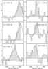 |
Fig. 4 Same as Fig. 2 for the remaining galaxies. |
| In the text | |
|
Fig. 5 Peak Tb ratio between the CO(3−2) and CO(1−0) lines versus the H2 density, and the CO column density per unit velocity width (NCO/ΔV) for two values of the kinetic temperature: Tk = 45 K, the dust temperature (left), and Tk = 20 K (right). The black contours are underlining the values obtained in the data. The predictions come from the LVG hypothesis in the Radex code. |
| In the text | |
|
Fig. 6 Measured CO luminosities, corrected for amplification when known, but not for gas excitation, as a function of redshift. We compare our points (full black circles, and arrows as upper limits) with a compilation of high-z molecular gas surveys, and local ones: green triangles are from Gao & Solomon (2004), blue squares from Solomon et al. (1997), open circles from Chung et al. (2009), blue diamonds from Geach et al. (2009), black crosses from Iono et al. (2009), red stars, from Greve et al. (2005), green full circles from Daddi et al. (2010), blue asterisks from Genzel et al. (2010), and blue full circles from Solomon & vanden Bout (2005). For illustration purposes only, the red curve is the power law for ΩH2/ΩHI proposed by Obreschkow & Rawlings (2009). |
| In the text | |
|
Fig. 7 Correlation between FIR and CO luminosities, for our sample (full black circles, and arrows for upper limits) and the other points from the literature (same symbols as in Fig. 6). The 3 lines are for LFIR/M(H2) = 10, 100 and 1000 L⊙/M⊙ from bottom to top, assuming a conversion factor α = 0.8 M⊙ (K km s-1 pc2)-1. The three lines correspond to gas depletion time-scales of 580, 58 and 5.8 Myr respectively. |
| In the text | |
|
Fig. 8 Optical color images from the Sloan Digital Sky Survey (SDSS, http://www.sdss.org/) of 15 of our sources. They are all detections, except G10 and G21. Each panel is 50′′ × 50′′ in size, and is centered on the galaxy coordinates of Table 1. |
| In the text | |
|
Fig. 9 Star formation efficiency SFE = LFIR/M(H2), versus CO luminosity, assuming the same CO-to-H2 conversion factor α = 0.8 M⊙ (K km s-1 pc2)-1. All symbols are as defined in Fig. 6. |
| In the text | |
|
Fig. 10 The star formation rate (SFR) obtained from the far infrared luminosity, versus the stellar mass of galaxies in our sample (full black circles), compared to the sample of Da Cunha et al. (2010, full red squares) and Fiolet et al. (2009, full green triangles). |
| In the text | |
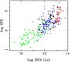 |
Fig. 11 Same as Fig. 9, but versus LFIR. |
| In the text | |
|
Fig. 12 Same as Fig. 9, but versus Td, for the sources where it could be defined. For the submillimeter galaxies, the red star corresponds to the averaged SFE, with the mean dust temperature of 35.5 found by Kovacs et al. (2010). |
| In the text | |
|
Fig. 13 Same as Fig. 9, but versus redshift. The red curve is a schematic line summarizing the cosmic star formation history, from the compilation by Hopkins & Beacom (2006), complemented with the GRB data by Kistler et al. (2009) and the optical data from Bouwens et al. (2008). The red curve is logarithmic and only indicative of relative variations of the star formation rate per cubic Mpc as a function of redshift, and can be translated vertically. |
| In the text | |
Current usage metrics show cumulative count of Article Views (full-text article views including HTML views, PDF and ePub downloads, according to the available data) and Abstracts Views on Vision4Press platform.
Data correspond to usage on the plateform after 2015. The current usage metrics is available 48-96 hours after online publication and is updated daily on week days.
Initial download of the metrics may take a while.