| Issue |
A&A
Volume 528, April 2011
|
|
|---|---|---|
| Article Number | A77 | |
| Number of page(s) | 11 | |
| Section | Astrophysical processes | |
| DOI | https://doi.org/10.1051/0004-6361/201014448 | |
| Published online | 04 March 2011 | |
Stellar mixing
II. Double diffusion processes⋆
1 NASA, Goddard Institute for Space
Studies, New
York, NY 10025, USA
2 Department of Applied Physics and
Applied Mathematics, Columbia University, New York, NY
10027,
USA
e-mail: This email address is being protected from spambots. You need JavaScript enabled to view it.
Received: 17 March 2010
Accepted: 25 August 2010
Abstract
In this paper, salt − fingers (also called thermohaline convection) and semi-convection are treated under the name of double − diffusion (DD). We present and discuss the solutions of the RSM (Reynolds stress models) equations that provide the momentum, heat, μ fluxes, and their corresponding diffusivities denoted by Km,h,μ. Such fluxes are given by a set of linear, algebraic equations that depend on the following variables: mean velocity gradient (differential rotation), temperature gradients (for both stable and unstable regimes), and μ-gradients (DD). Some key results are as follows. Salt − fingers. When shear is strong and DD is inefficient, heat and μ diffusivities are identical. Second, when shear is weak Kμ > Kh and the difference can be sizeable O(10) meaning that heat and μ diffusivities must therefore be treated as different. Third, for strong-to-moderate shears and for Rμ less than 0.8, both heat and μ diffusivities are practically independent of Rμ. Fourth, the latter result favors parameterizations of the type  suggested by some authors. Our results, however, show that C is not a constant but a linear function of the Reynolds number Re = ε(νN2)-1 defined in terms of the kinematic viscosity ν, the Brunt-Väisälä frequency N, and the rate of energy input into the system, ε. Fifth, we suggest that ε is an essential ingredient that has been missing in all diffusivity models, but which ought to be present because without a source of energy, turbulence dies out and so does the turbulent mixing (for example, the turbulent kinetic energy is proportional to the power 2/3 of ε). Moreover, since different stellar environments have different ε, its presence is necessary for differentiating mixing regimes in different stars. Semi − convection. In this case the destabilizing effect is the T-gradient, and when shear is weak, Kh > Kμ. Since the model is symmetric under the change Rμ to
  , most of the results obtained in the previous case can be translated to this case.
Key words: turbulence / diffusion / convection / hydrodynamics / methods: analytical / stars: rotation
This work is dedicated to Aura Sofia Canuto.
© ESO, 2011
1. Introduction
Double-diffusion (DD) processes (e.g., semi-convection and salt fingers) are import mixing mechanisms, for example, in low-mass red giants (e.g., Eggleton et al. 2006; Charbonnel & Zahn 2007; Denissenkov & Pinsonneault 2008; Cantiello & Langer 2008; Cantiello 2010; Denissenkov 2010). For lack of better models, these processes have thus far been quantified with either empirical relations or results from linear stability analysis, or both. The first methodology has obvious limitations, while the second faces the following problems.
First, linear analyses cannot fix amplitudes, and that explains why most of the results are presented as “ratios” in which amplitudes cancel out, for example, the heat-to-salt flux ratio in the ocean. A satisfactory comparison of such ratio vs. laboratory data (as in the salt-fingers case) is a welcome feature but is no assurance that each individual flux is reliable; and yet, what is required in the astrophysical case are the individual fluxes themselves. Second, though based on the results of dynamic equations, results of linear analysis run the risk of overestimating the efficiency of the DD processes. In stars, DD processes do not occur as they do in laboratory conditions chosen to highlight the DD processes alone where there is no shear. Stellar environments contain shear, which is known to disrupt salt fingers.
Third, none of the DD models based on linear stability analysis (or 2D simulations, Denissenkov 2010) has included shear; this amounts to assuming that the effect of shear is negligible or that the Richardson number is large. However, since when Ri < 1 (strong shear), DD processes are considerably weakened, assuming that shear is unimportant is risky at best.
However, we suggest that the most conspicuous shortcoming of all the models proposed thus far is the absence of a physically key ingredient, the energy required to sustain any type of turbulent motion. The conceptual underpinning of all models begins with the search for an instability that occurs when Re ≈ Re(cr), where Re is the Reynolds number, a process that is ordinarily carried out using linear stability analysis. The next step is to realize that when the instabilities grow, and Re ≫ Re(cr), the treatment requires the inclusion of nonlinearities, a feature that is outside the purview of linear models. Nonlinearities, while difficult to treat, have an interesting property: their volume integral is zero, and so they do no generate or destroy energy: they merely distribute whatever energy is available among the different scales.
Since energy is only distributed but not consumed, the energy input into the system percolates unchanged all the way to the smallest scales where irreversible processes such as kinematic viscosity and radiative losses degrade it into heat. That is why such the energy input equals the dissipation rate, usually denoted by ε (cm2 s-3). Without such power, there would be no turbulent motion or, equivalently, turning such power off would lead to a decaying turbulence and ultimately to no mixing. The well-known Kolmogorov law E(k) = Koε2/3 k − 5/3, which gives the kinetic eddy spectrum generated by the nonlinear interactions, contains ε, which varies from system to system, while the k-dependence of the spectrum has a universal character. Thus, since ε is not and cannot be a universal value and different stellar interiors have different power sources, its presence would ensure that different stellar interiors are characterized by different intensities of mixing. Diffusivity models that do not contain ε lack, in our opinion, a key physical ingredient.
Since the combination (N is the Brunt-Väisälä frequency1),  (1a)has the dimensions of a diffusivity, and the ratio of (1a) to the kinematic viscosity ν is the Reynolds number
  (1b)one might conclude that the diffusivities Kα (the subscript α stands for momentum, heat, passive tracer, etc.) in units of the radiative value χ (cm2 s-1) are given by the relation:
 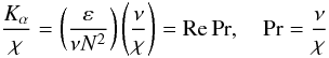 (1c)where Pr is the Prandtl number, which may be as small as 10-7 in stellar interiors. A concrete example may help. Consider a fully convective, unstably stratified regime N2 < 0, in which nearly the entire outward flux is carried by convective motion. In a steady state, where production balances dissipation, we have for the Rμ = 0 case
  (1d)and thus
  (1e)which shows that (1a) is the physically correct combination to express the diffusivity2. On the other hand, while convection leading to (1e) is an extremely efficient limiting case without competing effects, in regimes with N2 > 0 (stable stratification) mixing may come from: a) shear; b) differential rotation; c) μ-gradients while T-gradients work against it (salt fingers); and d) T-gradients while μ-gradients work against it (semi-convection). In such circumstances, one must account for competing effects, which means that there must be a “mixing efficiency”, usually denoted by Γ, with generalizes (1e) to
  (1f)and thus
 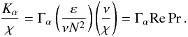 (1g)As we shall prove below, the RSM (Reynolds stress models) not only give rise to exactly expression (1f), which we arrived at above using heuristic arguments, but it further provides the full form of the dimensionless functions Γ
 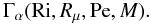 (1h)Here, Ri is the Richardson number (measuring the competing effect on the mixing generated by shear and the opposite effect due to stable stratification), Rμ is the density ratio (which measures the DD processes), Pe is the Peclet number defined in (5b), which measures the effect of radiative losses and M represents meridional currents. Using the general expression (1g), in Sect. 5.1), we show how all previous models have essentially guessed the form of the function (1h) by neglecting all dependences except the one on Rμ, see for example, Eqs. (15d, e). At the same time, they took the Re Pr dependence to be a constant C, an assumption that cannot be valid since, as just discussed, this is a key variable that depends on the particular star one is considering. Relations (1g), (1h) resulting from the RSM model are shown in Figs. 1–3. The Ri dependence in (1h) requires comments. First, its definition is
  (1i)where
  represents the mean flow velocity and Sij the shear. Stable and/or unstable regimes are characterized by the relations
  (1j)The first regime corresponds to a density profile that decreases with height, while the second regime corresponds to one in which the density profile increases with height as in thermal convection. Next, consider the conditions for semi-convection and salt-finger regimes.

 (1k)
(1k)

 (1l)Oceanic salt fingers correspond to warm-salty over cold-fresh water, a regime in which the z-gradients of T and S are positive. Though the T-gradient is stable and the S-gradient unstable, the overall N2 is positive, corresponding to a stably stratified regime. The Mediterranean Sea is a known example of such a regime. A semi-convection regime, which in oceanography is called diffusive-convection, corresponds to cold-fresh over warm-salty water. Both T − S gradients are negative, but N2 is positive corresponding to a stably stratified regime. A typical example is water under ice. In what follows, we present the algebraic 3D solutions of the RSM that provide the ingredients needed to construct Γh,μ. In Sect. 3.6, we work out a physical representation of Γh,μ that exhibits the shear and DD contributions in a fairly transparent way.
2. Stresses and fluxes
For completeness, we summarize the relevant equations that we have derived in Paper I and that correspond to the local, stationary case.
Reynolds stresses:  (2a)Vorticity tensor:
  (2b)Buoyancy tensor:
  (2c)Buoyancy-density flux:
 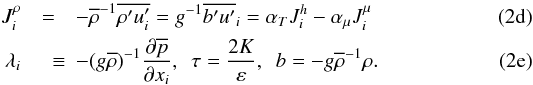 It is easy to check that all the above tensors are traceless.
Heat fluxes: 
![Mathematical equation: \begin{equation} \label{eq15} \begin{array}{l} \gamma _{ij} = \pi _4 \tau (R_{ij} -\pi _2 g\alpha _\mu \tau \lambda _i J_j^\mu) \\ \eta _{ij} =\pi _4 \tau [S_{ij} +V_{ij} -g\tau \lambda _i (\pi _5 \alpha_T \beta _j +\pi _2 \alpha _\mu \overline \mu _{,j} )]. \\ \end{array} \end{equation}](/articles/aa/full_html/2011/04/aa14448-10/aa14448-10-eq69.png) (3)μ-fluxes:
(3)μ-fluxes:  :
: ![Mathematical equation: % subequation 944 0 \begin{eqnarray} \label{eq16} (\delta _{ij} +\xi _{ij} )J_j^\mu &=& - d_{ij} \overline \mu _{,j} \nonumber\\ d_{ij} &=& \pi _1 \tau (R_{ij} +\pi _2 g\alpha _T \tau \lambda _i J_j^h)\nonumber \\ \xi _{ij} &=& \pi _1 \tau [S_{ij} +V_{ij} -g\tau \lambda _i (\pi _2 \alpha _T \beta _j +\pi _3 \alpha _\mu \overline \mu _{,j} )] \end{eqnarray}](/articles/aa/full_html/2011/04/aa14448-10/aa14448-10-eq71.png) (4a)where:
(4a)where:  (4b)Dissipation-relaxation times scales:
 ![Mathematical equation: % subequation 969 0 \begin{eqnarray} \label{eq18} \pi _1 &=& \pi _1^0 \left(1 + \frac{{\rm Ri} R_\mu}{a + R_\mu }\right)^{-1}, \pi _4 = \pi _4^0 f({\rm Pe}) \left( 1 + \frac{\rm Ri}{1 + aR_\mu} \right)^{-1} \nonumber\\ \pi _2 &=& \pi _2^0 (1+{\rm Ri})^{-1} [1+ 2 {\rm Ri} R_\mu (1+R_\mu ^2 )^{-1}], \pi _5 =\pi _5^0 g({\rm Pe}), \nonumber\\ \pi _1^0 &=&\pi _4^0 =(27~{\rm Ko}^3/5)^{-1/2}(1+\sigma _t^{-1} )^{-1},\nonumber\\ \pi _2^0 &=& 1/3, \pi _3 =\pi _3^0 = \pi _5^0 =\sigma _t \nonumber\\ f({\rm Pe}) &=& b{\rm Pe} (1+b{\rm Pe})^{-1},\quad g({\rm Pe}) = c{\rm Pe}(1 + c{\rm Pe})^{-1},\nonumber \\ a&=&10, {\rm Ko} = 5/3,\; 4 \pi ^2b=5(1+\sigma _t^{-1} ),\;7\pi ^2c=4\sigma _t^{-1}. \end{eqnarray}](/articles/aa/full_html/2011/04/aa14448-10/aa14448-10-eq73.png) (5a)Here, Pe is the Peclet number representing radiative losses,
(5a)Here, Pe is the Peclet number representing radiative losses,  (5b)where χ (cm2 s-1) = Kr(cpρ)-1 is the thermometric conductivity, Kr = 4acT3(3ρκ)-1 is the radiative diffusivity, and κ is the opacity. In the previous relations, K, ε, and τ are the eddy kinetic energy, its rate of dissipation, and the dynamical time scale, which are related to one another as follows
  (5c)
(5c)
3. The 1D case. Solutions of Eqs. (2–4)
Since Eqs. (3–5) are algebraic relations, in the 1D case the solutions representing the heat, concentration and momentum fluxes have a particularly simple form:  (6a)where Kh,μ,m are the T, μ and momentum diffusivities The simplest representation that that emerges from solving the rms equations is (see Eq. C.1 of Paper I)
 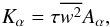 (6b)where
  is twice the vertical component of the eddy kinetic energy and the Aα are dimensionless functions discussed below. Using the representation (1f), we find
  (6c)where the functions Aα and
  are given next. In Sect. 3.6, we work out a representation of Γh,μ that exhibits the shear and DD contributions in a transparent way.
3.1. Dimensionless structure functions Aα
The solution of the RSM yields the following results: ![Mathematical equation: % subequation 1037 3 \begin{eqnarray} \label{eq23} A_h &=& \pi _4 [1+ px + \pi _2 \pi _4 x(1-r^{-1})]^{-1}, \nonumber\\ A_\mu &=& A_h (rR_\mu )^{-1}, A_m =\frac{A_{m1} }{A_{m2}}, \end{eqnarray}](/articles/aa/full_html/2011/04/aa14448-10/aa14448-10-eq90.png) (6d)where
(6d)where ![Mathematical equation: % subequation 1037 4 \begin{eqnarray} \label{eq24} A_{m1} &=& \frac{4}{5} - \left[ \pi _4 -\pi _1 + \left(\pi _1 -\frac{1}{150}\right) (1-r^{-1})\right] xA_h ,\nonumber\\ A_{m2} &=& 10+ (\pi _4 -\pi _1 R_\rho )x+\frac{1}{50}(\tau \Sigma)^2. \end{eqnarray}](/articles/aa/full_html/2011/04/aa14448-10/aa14448-10-eq91.png) (6e)The solution of the Reynolds Stresses yields the following result
(6e)The solution of the Reynolds Stresses yields the following result
General case: ![Mathematical equation: % subequation 1037 5 \begin{eqnarray} \frac{\overline {w^2}}{2K} = \frac{1}{3}\left[1+\frac{2}{15}A_\rho (\tau N)^2+\frac{1}{10}A_m (\tau \Sigma )^2\right]^{-1} \end{eqnarray}](/articles/aa/full_html/2011/04/aa14448-10/aa14448-10-eq92.png) (6f)
(6f)
![Mathematical equation: % subequation 1037 6 \begin{eqnarray} P&=& \varepsilon\\ \frac{\overline{w^2}}{2K} &=& \left[\frac{30}{7} + A_\rho (\tau N)^2 \right]^{-1}, \end{eqnarray}](/articles/aa/full_html/2011/04/aa14448-10/aa14448-10-eq93.png)
where we have defined the following dimensionless functions: The model results are as follows:
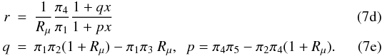
3.2. The variable (τ N)2. Nonlocal model
As discussed in Paper I, Sect. 6, since the dynamical time scale defined in (5c) depends on the kinetic energy and on its rate of dissipation, one must solve two dynamic equations for K and ε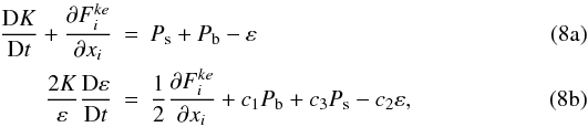 where using (6a), the production due to shear and buoyancy are given by
 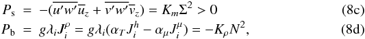 where the density diffusivity is defined as
 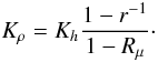 (8e)When the heat and concentration diffusivities are the same, Eq. (7b) gives
  and (8e) yields Kρ = Kh = Kμ, as expected. The flux of eddy kinetic energy
  was commented upon in Sect. 6 of Paper I and will be discussed again in Paper V.
3.3. The variable (τ N)2. Local model P = ε
If instead of solving the nonlocal model (8a, b), with the diffusion terms represented by the fluxes of K and ε, we assume a local model where production is equal dissipation, the model simplifies considerably. While the Ah,μ remain the same, the expression for Am simplifies to ![Mathematical equation: % subequation 1262 0 \begin{equation} \label{eq35} A_m = \frac{2}{(\tau \Sigma )^2}\left[\frac{15}{7} + A_\rho (\tau N)^2\right]. \end{equation}](/articles/aa/full_html/2011/04/aa14448-10/aa14448-10-eq106.png) (9a)In the local limit, Eq. (8a) becomes
(9a)In the local limit, Eq. (8a) becomes  (9b)Using the notation first introduced by Mellor & Yamada (1982)
  (9c)Equation (9b) becomes, after a great deal of algebra, the following equation for Gm in terms of Ri , Rρ, and Pe
  where the functions Ak are given in Appendix A, Eq. (A.3).
3.4. Dissipation rate, Reynolds number
As already noted, the advantage of the representation (1f,g) is that it highlights the role of the power available to generate a mixing state, the degree of stratification N2 and the role of χ. Clearly, different physical environments have quite different Re because the power to generate mixing can be of quite different nature. In addition to the example of convection in Eqs. (1d–e), we can consider the region below the CZ, where an estimate of ε was presented by Kumar et al. (1999) and which represents the power of internal gravity waves. Their results is  (10a)If we employ typical values N2 = 10-7 s-2 and χ = 109 cm2 s-1 from the second and third relations in (1g), we obtain
  (10b)which is one of the values we considered in presenting the results of our model in Figs. 1–4. To gain an appreciation of what (10b) implies, consider a realistic Prandtl number of Pr = ν/χ = 10-7. The Reynolds number then becomes
  (10c)The value (10c) shows that, below the CZ, turbulence is only moderately strong, as one indeed expects from general considerations. However, since our model is valid in general, we present the results for different Re since different stellar environments have different values of ε than in (10a). Instead of Re could we have labeled the figures with Pe? The answer is negative since Pe is not an outside variable, such as N2,χ,ε but an internal dynamical variable that depends on the turbulent kinetic energy and as such, it is determined internally as part of the solution of the problem. Pe is therefore an output, not an input, which implies that it cannot be assumed to be a fixed value since it is a dynamical variable. That makes the comparison with numerical simulations difficult since they treat Pe as fixed. For example, Fig. 14 of Brummel et al. (2002) shows that, unless Pe is very large, the resulting “overshooting measure” would exceed the helio-seismic data of ~0.1 Hp (cited in the Discussion section of the above reference) by an order of magnitude. Specifically, in order to bring their OV extent into the range of the helio data, Brummel et al. (2002) had to invoke a value of Pe about 100 times larger than what they used, that is, a value of Pe ~ 104. Such a value is predicted by the present model as one can see from Figs. 1–3 but, as before, other conditions must be satisfied, namely,
  (10d)which is quite restrictive since it seems to exclude the bottom of the convective zone and the underlying shear dominated tachocline.
3.5. Peclet number dependence
The determination of Pe that enters the time scales Eq. (5a) begins with the definition (5b), which we rewrite as  (10e)and which shows that Pe is not a fixed number but a dynamical variable that depends on Ri, Re, Rμ; that is,
  (10f)corresponding to arbitrary T and μ-gradients, arbitrary shear, and Reynolds number. Relation (10f) naturally complicates the solution of Eq. (9d) since the coefficients A1,...6 in (9e) depend on the πk which in turn depend on Pe, which itself depends on the unknown function Gm. For large values of Pe corresponding to negligible radiative losses, the πk are practically independent of Pe, and the solution of Eq. (9d) is simplified. It is only when radiative losses are important and Pe is small that the solution of Eq. (9d) becomes more involved and requires an iterative process.
In conclusion, the diffusivities of heat, μ, and momentum measured in units of χ, are given by Eqs. (1f, g) and (6c). Since the amount of energy needed to generate the turbulent state is an outside parameter, it is physically correct to consider the variable RePr as an external parameter, and for this reason in Figs. 1–3, we present the results for different values of such variable, that is, the diffusivities are functions of  (10g)The Richardson number Ri represents the competition between stable stratification (a sink of mixing) and shear (a source of mixing), Rμ represents DD processes and Re represents the amount of energy dissipated. The nonexistence of a critical Richardson number was discussed in Paper I and in Canuto et al. (2008a).
 |
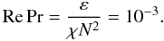
Fig. 1 No doublediffusion, shear only. The heat, momentum, and μ mixing efficiencies, as defined in Eq. (1f), vs. Ri for different values of the combination RePr which in the figures is denoted by Reχ. In Fig. 1d we plot the turbulent Prandtl number σt defined in Eq. (14) vs. Ri for different Reχ. In Fig. 1e we plot the Peclet number vs. Ri. In Fig. 1f we plot the data corresponding to the case Pe ≫ 1, which well reproduced well by the present model, lower curve in panel 1e. The data are as follows: meteorological observations (Kondo et al. 1978, slanting black triangles; Bertin et al. 1997, snow flakes), lab experiments (Strang & Fernando 2001, black circles; Rehmann & Koseff 2004, slanting crosses; Ohya 2001, diamonds), LES (Zilitinkevich et al. 2007a,b, triangles), DNS (Stretch et al. 2001, five-pointed stars). |
3.6. Alternative representation of Γh,μ
Though relations (1g) and (6c) are the basic relations for computing the various diffusivities, it is instructive to present an expression for Γh,μ that exhibits the shear and DD contributions in a transparent way. Let us begin by taking the rhs of (8a) as zero which corresponds to the local model production = dissipation. Use of relations (8c, d) in the Ps + Pb = ε relation leads to 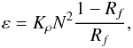 (10h)where the flux Richardson number is defined as
 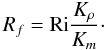 (10i)Next, using Eq. (8e), we obtain the desired expression for
  which is
 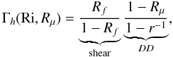 (10j)which exhibits the dependence on shear (Ri) and DD (Rμ). Consider some limiting cases. In the presence of strong shear, heat and μ, diffusivities become equal, and from (7b) we have . Relation (10j) then becomes the well-known expression
Strong shear (No DD):  (10k)where the turbulent Prandtl number σt(Ri) is known to be an increasing function of Ri as Fig. 1f shows. Conversely, in the absence of shear, Rf → ∞, relation (10j) becomes No shear (DD):
 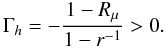 (10l)In the salt fingers case, one has Rμ < 1,r < 1 which yields a positive Γh. In the semi-convective regime, Rμ > 1, r > 1 and Γh > 0. Finally, the expression for Γμ is
 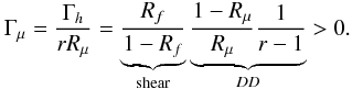 (10m)There is only one set of data from the North Atlantic Tracer Release Experiment (NATRE, Ledwell et al. 1993, 1998) that provide the function
  (10n)in the presence of both DD (salt fingers) and shear. Such data (St. Laurent & Schmitt 1999) were used to test relation (10j) or, more specifically, the model used to evaluate the different terms in it. The model presented in Sects. 3.1–3.3 was found to reproduce such data well (Canuto et al. 2008b).
4. Ledoux vs. Schwarzschild criteria for semi-convection
In the case of semi-convection, the Ledoux & Schwarzschild criteria are often discussed as if they were antithetic, implying an uncertainty in the choice of one of the two. To discuss the topic, let us consider the case of no shear, and thus the second of (9b) implies that
 If we consider the mass flux, we see that, using (2d) we find
 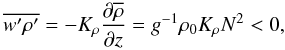 (11c)which corresponds to a downward mass flux. We distinguish several regimes of interest: Semi-convection, Ledoux stable, Rμ > 1,N2 > 0. From (11b) we obtain
  (11d)Dynamical stability (∇μ > ∇ − ∇ad) sets the lower limit of ∇μ and does not depend on any characteristics of turbulent mixing, while the latter sets the upper limit. The Schwarzschild instability criterion ∇ − ∇ad > 0 corresponds to rewriting (11c) as
 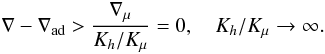 (11e)However, the last relation is not satisfied in any known regime.
Semi-convection, Ledoux unstable, Rμ < 1,N2 < 0. In this case we have  (12a)Salt-fingers, Ledoux stable, Rμ < 1,N2 > 0. In this case we have
  (12b)Salt-fingers, Ledoux unstable, Rμ > 1,N2 < 0. In this case we have
  (12c)Thus, in summary, we have:
 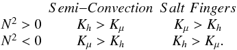 (12d)
(12d)
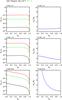 |
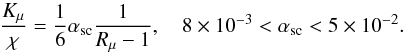
Fig. 2 Salt fingers. The normalized diffusivities Kh,μ/χ vs. Rμ < 1, for different values of Ri and RePr ≡ Reχ. See relation (1g). |
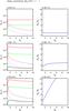 |
Fig. 3 Semi convection. Same as Fig. 2 but for Rμ > 1. The dash-dotted curves represent the empirical relation (15h). |
5. Results
The formalism presented above shows that the diffusivities depend on three parameters, namely, 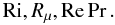 (13)We have numerically solved the 1D model in the local limit P = ε, Appendix C, and the results are shown in Figs. 2–3 where we present the heat, momentum, and μ diffusivities in units of the thermometric diffusivity, χ, defined after Eq. (5b), as a function of Rμ for different values of RePr and Ri. We recall that salt fingers and semi-convection are represented by Rμ < 1, Rμ > 1 respectively, see Eqs. (1k, l). For completeness, for the Rμ = 0 case, we also present the Peclet number Pe, Eqs. (5b, 10e), and the turbulent Prandtl number:
  (14)As expected, the ratio (14) is not constant but increases with Ri, a feature that the model predicts since it is physically clear that stable stratification affects temperature more than velocity, and thus it lowers the heat diffusivity more than the momentum one, yielding a σt that increases with Ri, as is indeed observed. For the large Pe regime, the model reproduces the available data discussed in Canuto et al. (2008) and presented in Fig. 1f well. As expected, the stronger the radiative losses, represented by small values of RePr, the smaller the heat diffusivity, first panel in each figure.
5.1. Results
No DD. In this case, all the mixing models used thus far in stellar structure calculations (e.g., Mathis et al. 2004; Palacios et al. 2003, 2006; Charbonnel & Talon 2005, 2007) assume the existence of a finite Ri(cr) since their starting point is the relation  (15a)which ultimately gives
  (15b)since Ri(cr) was taken to be 1/6 (Maeder & Meynet 2001). As stated by the previous authors, relations (15a,b) are only valid in the absence of “thermal leakage” that is, for Pe ≫ 1. The first remark is that the basis of this model, Eq. (15a), disagrees with the data shown in Fig. 1f since there is no Ri(cr), see Canuto et al. (2008a). Let us, however, assume for a moment that (15b) was arrived at in a way that does not involve the existence of Ri(cr); that is, consider it an heuristic relation and compare it with the results of the model. From Figs. 1d, e, we observe that the equality of momentum and heat diffusivities can be satisfied only under the conditions
  (15c)The problem is not so much the validity of (15b), but rather how legitimate it is to use (15b) in regimes of Ri, Pe, and RePr other than those described in (15c). Salt fingers (thermohaline convection). The relevance of this process was recognized quite early (Stothers & Simon 1969), but even today its modeling is still based on largely heuristic relations, the first of which was proposed by Ulrich et al. (1972) and used by several authors (Kippenhahn et al. 1980; Vauclair 2004, 2008; Eggleton et al. 2006; Charbonnel & Zahn 2007). The Ulrich model for the ratio Kh/χ reads
  (15d)where r is the ratio of heat-to-μ fluxes, see Eq. (7b). The value of C has been a matter of debate: Cantiello & Langer (2008, 2010) use C = 3, while Charbonnel & Zahn (2007) use C = 658. A different relation,
  (15e)was used by Denissikov and Pinsonneault (2008) to reproduce data for low-mass RGB stars. Relation (15d) with C = 3, 1000 are consistent with (15e) for Rμ ≃ 10-2,10-5 respectively, so these models cannot be ruled out. However, due to a difference of a factor of a thousand in their values of Rμ, the two models must have different implications. The results presented in Fig. 2 exhibit interesting features. Since in this case, the destabilizing effect comes from the μ gradient, in Fig. 2 we plot Kμ/χ for the following parameters
  (15f)
(15f)
- a)
For strong shear, e.g., Ri = 0.1,there is little difference between heat and μ diffusivities, as indeed expected;
when shear is weak, e.g., for Ri = 10, panel f) shows that the μ diffusivity is larger than the heat diffusivity, as expected, since in the salt-finger case, it is the μ field that causes the instabilities. The ratio Kμ/Kh may be significant, as one can observe in panel f). This implies that heat and μ diffusivities cannot be taken to be the same;
in each case the dependence on RePr = Reχ of Eq. (1g) is clearly seen.
in each of the panels on the rhs there is only one curve since the variable Reχ ≡ RePr cancels out in the ratioKμ/Kh;
the broad insensitivity on the density parameter Rμ up to values of about 0.8, for the case of strong-moderate shear favors models of the form (15e), but since such models have no Ri-dependence, it is more consistent to compare them with the results for small shear, large Ri of panel e);
contrary to (15e), the coefficient C is not a constant but a linear function of RePr;
if we regard (15e) as an empirical input, panel e) shows that it is reproduced by the RSM for Rμ ≪ 1 and for
 (15g)Using Fig. 2 of Denissenkov & Pinsonneault (2008) which yields Pr = O(10-6) and ν = O(102) cm2 s-1, one can then deduce a value for ε.
 (15h)Since in this case the destabilizing effect is the T-gradient, when shear is weak-to-moderate, Kh > Kμ, as shown in Fig. 3. Most of the conclusions of the salt-finger case can be repeated here since the model is symmetric under the change Rμ to . In conclusion, in both salt-finger and semi-convection regimes, the present model yields a dependence of the ratio Kμ/χ on the variables:
 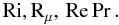 (15i)Heuristic mixing models such as (15d), (15e), and (15h) have focused only on the Rμ dependence, while neglecting the dependence on
  (15j)which they assume to be a constant, e.g., C and/or αsc/6 in the previous relations, while in reality it is a key factor since it determines the strength of the ratios Kh,μ/χ, and it varies from star to star.
6. Conclusions
A welcome feature of the RSM is the relative simplicity of the equations determining the Reynolds stresses, heat and μ fluxes. The presence of two differential equations for K and ε is a common features of all turbulence models. When a local model is applicable, the present model is fully algebraic and yet the amount of information these relations contain is quite substantial: stable stratification, unstable stratification, rigid rotation, shear, and radiative losses (Peclet number).
We recall the relations  , Rμ = ∇μ(∇ − ∇ad)-1,
  ,
, ![Mathematical equation: \hbox{$\alpha _T [-\overline T _{,z} +(\overline T _{,z} )_{\rm ad}] = H_{\rm p}^{-1} (\nabla - \nabla_{\rm ad})$}](/articles/aa/full_html/2011/04/aa14448-10/aa14448-10-eq241.png) ,
,  ,
,  .
.
We recall that L/M|sun = O(1) cm2 s-3 ~ 10-4 W/kg,L|sun ~ 1026 W(W = Watts); in the convective zone, the mixing length theory gives  where ℓ = αpHp. In the middle of the solar CZ, ε ≈ 35 cm2 s-3 (solar code courtesy of Mazzitelli). Below the CZ, the internal gravity waves give ε(IGW):10-3 cm2 s-3 (Kumar et al. 1999).
References
- Brummel, N. H., Clune, T. L., & Toomre, J. 2002, ApJ, 570, 865 [NASA ADS] [CrossRef] [EDP Sciences] [Google Scholar]
- Cantiello, M., & Langer, N. 2008, in IAU Symp. 252, ed. Deng, L. & Chan, K. L. (Cambridge Univ. Press), 83, 103 [Google Scholar]
- Cantiello, M., & Langer, N. 2010, A&A, 521, A9 [NASA ADS] [CrossRef] [EDP Sciences] [Google Scholar]
- Canuto, V. M. 1999, ApJ, 524, 311 [NASA ADS] [CrossRef] [Google Scholar]
- Canuto, V. M., Cheng, Y., Howard, A., & Esau, I. N. 2008a, J. Atmos. Sci., 65, 2437 [NASA ADS] [CrossRef] [Google Scholar]
- Canuto, V. M., Cheng, Y., & Howard, A. M. 2008b, Geophys. Res. Lett., 35, L02613 [Google Scholar]
- Charbonnel, C., & Talon, S. 2005, Science, 309, 2189 [NASA ADS] [CrossRef] [PubMed] [Google Scholar]
- Charbonnel, C., & Talon, S. 2007, Science, 318, 922 [CrossRef] [PubMed] [Google Scholar]
- Charbonnel, C., & Zahn, J. P. 2007, A&A, 467, L15 [NASA ADS] [CrossRef] [EDP Sciences] [Google Scholar]
- Denissenkov, P. A. 2010, ApJ, 723, 563 [NASA ADS] [CrossRef] [Google Scholar]
- Denissenkov, P. A., & Pinsonneault, M. 2008, ApJ, 684, 626 [NASA ADS] [CrossRef] [Google Scholar]
- Eggleton, P. P., Dearborn, D. S. P., & Lattanzio, J. C. 2006, Science, 314, 1580 [NASA ADS] [CrossRef] [PubMed] [Google Scholar]
- Kippenhahn, R., Ruschenplatt, G. & Thomas, H. C. 1980, A&A, 91, 175 [NASA ADS] [Google Scholar]
- Kondo, J., Kanechika, O., & Yasuda, N. 1978, J. Atmos. Sci., 35, 1012 [NASA ADS] [CrossRef] [Google Scholar]
- Kumar, P., Talon, S., & Zahn, J. P. 1999, ApJ, 520, 859 [NASA ADS] [CrossRef] [Google Scholar]
- Langer, N., El Eid, M. F., & Baraffe, I. 1989, A&A, 224, L17 [NASA ADS] [Google Scholar]
- Ledwell, J. R., Watson, A. J., & Law, C. S. 1993, Evidence for slow mixing across the pycnocline from open ocean tracer release experiment, Nature, 364, 701 [NASA ADS] [CrossRef] [Google Scholar]
- Ledwell, J. R., Wilson, A. J., & Law, C. S. 1998, Mixing of a tracer released in the pycnocline of a subtropical gyre, J. Geophys. Res., 103, 21499 [NASA ADS] [CrossRef] [Google Scholar]
- Maeder, A., & Maynet, G. 2001, A&A, 373, 555 [NASA ADS] [CrossRef] [EDP Sciences] [Google Scholar]
- Mathis, S., Palacios, A., & Zahn, J. P. 2004, A&A, 425, 243 [NASA ADS] [CrossRef] [EDP Sciences] [Google Scholar]
- Palacios, A., Talon, S., Charbonnel, C., & Forestini, M. 2003, A&A, 399, 603 [NASA ADS] [CrossRef] [EDP Sciences] [Google Scholar]
- Palacios, A., Charbonnel, C., Talon, S., & Seiss, L. 2006, A&A, 453, 261 [NASA ADS] [CrossRef] [EDP Sciences] [Google Scholar]
- St. Laurent, L., & Shmitt, R. W. J., Phys. Oceanogr., 29, 1404 [Google Scholar]
- Stothers, R., & Simon, R. N. 1969, ApJ, 157, 673 [NASA ADS] [CrossRef] [Google Scholar]
- Ulrich, R. K. 1972, ApJ, 172, 165 [NASA ADS] [CrossRef] [Google Scholar]
- Vauclair, S. 2004, ApJ, 605, 874 [NASA ADS] [CrossRef] [Google Scholar]
- Vauciar, S. 2008, in IAU Symp. ed. L. Deng, & K. L. Chan (Press: Cambridge Univ.), 252, 83, 97 [Google Scholar]
Appendix A: The functions Ak in relation (9e)
We begin with relations (9d, e), which we rewrite here:  (A.1)with
  (A.2)The coefficients Ak are given by the following algebraic expressions:
 ![Mathematical equation: \appendix \setcounter{section}{1} \begin{eqnarray} 150(1-R_\rho )^3A_1 &=& \pi _1 \pi _4 (\pi _4 -\pi _1 R_\rho) \{ \pi _2 (15 \pi _3 +7)(R_\rho ^2 +1) \nonumber\\ &\quad +& [ 14 (\pi _2 - \pi _3 ) - 15 \pi _3^2 ] R_\rho \}\nonumber \\ 9000(1-R_\rho )^2A_2 &=&\pi _1 \pi _4 \{\pi _2 (210\pi _1 -150 \pi _3 +7)(R_\rho ^2 +1) \nonumber\\ &\quad +& [14(\pi _2 - \pi _3 )(1+15 \pi _1 \nonumber\\ &\quad +&15\pi _4 ) +150\pi _3^2]R_\rho + 210 \pi _2 (\pi _4 -\pi _1 )\} \nonumber \end{eqnarray}](/articles/aa/full_html/2011/04/aa14448-10/aa14448-10-eq205.png)
 \nonumber\\ &\quad -& (15\pi _3 +7)(\pi _1^2 -\pi _4^2 ) \nonumber\\ &\quad -&[10\pi _1 \pi _3 \pi _4 (15\pi _3 +17)\nonumber\\ &\quad +&15\pi _2 (\pi _1^2 + \pi _4^2 )+ 14 \pi _1 \pi _4 (1-10 \pi _2 )]R_\rho \nonumber \end{eqnarray}](/articles/aa/full_html/2011/04/aa14448-10/aa14448-10-eq206.png)
![Mathematical equation: \appendix \setcounter{section}{1} \begin{eqnarray} 9000(1-R_\rho )A_4 &=& [150(\pi _1 \pi _3 +\pi _2 \pi _4 ) \nonumber\\ &\quad -& 7\pi _1 (1+30\pi _1)]R_\rho \nonumber\\ &\quad -& 150(\pi _1 \pi _2 +\pi _3 \pi _4 )\nonumber\\ &\quad +&7\pi _4 (1+30\pi _4 )\nonumber \\ 30(1-R_\rho )A_5 &=& [-30(\pi _1 \pi _3 \nonumber\\ &\quad +& \pi _2 \pi _4 )\nonumber\\ &\quad -& 17\pi _1 ]R_\rho +30(\pi _1 \pi _2 +\pi _3 \pi _4 )+17\pi _4 ,\nonumber \end{eqnarray}](/articles/aa/full_html/2011/04/aa14448-10/aa14448-10-eq207.png)
 (A.3)
(A.3)
Appendix B: 3D Mixing model
Reynolds stresses:  (B.1)Momentum diffusivity and dynamical time scale:
  (B.2)Vorticity tensor:
  (B.3)Buoyancy tensor:
  (B.4)Buoyancy flux:
  Shear and vorticity:
  (B.7)Heat fluxes:
![Mathematical equation: \appendix \setcounter{section}{2} \begin{eqnarray} (\delta _{ij} +\eta _{ij} )J_j^h &=& \gamma _{ij} \beta _j \nonumber\\ \gamma _{ij} &=& \pi _4 \tau (R_{ij} -\pi _2 g \alpha _\mu \tau \lambda _i J_j^\mu) \nonumber\\ \eta _{ij} &=& \pi _4 \tau [S_{ij} +V_{ij} - g \tau \lambda _i (\pi _5 \alpha _T \beta _j + \pi _2 \alpha _\mu \overline \mu _{,j} )]. \end{eqnarray}](/articles/aa/full_html/2011/04/aa14448-10/aa14448-10-eq216.png) (B.8)μ-fluxes:
(B.8)μ-fluxes:  :
: ![Mathematical equation: \appendix \setcounter{section}{2} \begin{eqnarray} (\delta _{ij} +\xi _{ij} )J_j^\mu &=& - d_{ij} \overline \mu _{,j} \nonumber\\ d_{ij} &=& \pi _1 \tau (R_{ij} +\pi _2 g \alpha _T \tau \lambda _i J_j^h) \nonumber \\ \xi _{ij} &=& \pi _1 \tau [S_{ij} + V_{ij} - g \tau \lambda _i (\pi _2 \alpha _ T \beta _j +\pi _3 \alpha _\mu \overline \mu _{,j} )] \end{eqnarray}](/articles/aa/full_html/2011/04/aa14448-10/aa14448-10-eq219.png) (B.9)where
(B.9)where  (B.10)
Appendix C: 1D Mixing model with P = ε
Heat, concentration and momentum diffusivities (subscript α):  (C.1)Dimensionless structure functions:
 ![Mathematical equation: \appendix \setcounter{section}{3} \begin{eqnarray} S_\alpha &=& A_\alpha \frac{\overline {w^2} }{K}, \quad G_{\rm m} \equiv (\tau \Sigma)^2\\ A_h & = & \pi _4 [1+px+\pi _2 \pi _4 x(1-r^{-1})]^{-1},\nonumber\\ A_\mu & = & A_h (rR_\mu )^{-1} \\ A_m & = & \frac{2}{(\tau \Sigma)^2}\left[\frac{15}{7}+A_\rho (\tau N)^2\right] \end{eqnarray}](/articles/aa/full_html/2011/04/aa14448-10/aa14448-10-eq223.png) Heat to concentration flux ratio:
Heat to concentration flux ratio: 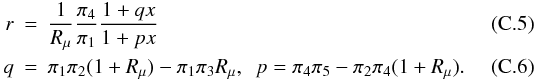 Ratio of vertical to total kinetic energy:
 ![Mathematical equation: \appendix \setcounter{section}{3} \begin{equation} \frac{1}{2}\frac{\overline {w^2} }{K}= \left[\frac{30}{7}+A_\rho (\tau N)^2\right]^{-1}. \end{equation}](/articles/aa/full_html/2011/04/aa14448-10/aa14448-10-eq225.png) (C.7)Dimensionless dynamical time scale:
(C.7)Dimensionless dynamical time scale: 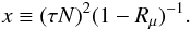 (C.8)Equation for Gm: see Eqs. (9d, e) Flux Richardson number:
  (C.9)Density structure function:
  (C.10)Turbulent Prandtl number:
  (C.11)Density ratio:
 ![Mathematical equation: \appendix \setcounter{section}{3} \begin{equation} R_\mu \equiv \frac{\alpha _\mu \overline \mu _{,z}}{\alpha _T [\frac{\partial \overline T }{\partial z}-(\frac{\partial \overline T }{\partial z})_{\rm ad} ]}=\frac{\nabla _\mu }{\nabla -\nabla _{\rm ad} }\cdot \end{equation}](/articles/aa/full_html/2011/04/aa14448-10/aa14448-10-eq231.png) (C.12)Richardson number:
(C.12)Richardson number:  (C.13)Brunt-Väisälä frequency:
 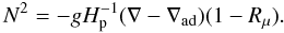 (C.14)Mean shear:
 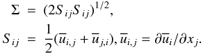 (C.15)Dimensionless time scales:
  (C.16)
![Mathematical equation: \appendix \setcounter{section}{3} \begin{eqnarray} \pi _2 &=& \frac{1}{3}\left[\frac{1}{2}(R_\mu +R_\mu ^{-1})\right]^{-1}, \quad\pi _5 = \pi _5^0 {g\rm (Pe)}, \nonumber\\ \pi _3 &=& \pi _3^0 = \pi _5^0 = \sigma _t, \qquad\pi _1^0 = \pi _4^0 =0.08, \nonumber\\ f{\rm (Pe)} &=& \frac{b\rm Pe}{1+b\rm Pe}, \quad {g\rm (Pe)} = \frac{c\rm Pe}{1+c\rm Pe}, \nonumber\\ (4\pi ^2)b&=&5(1+\sigma _t^{-1} ),\quad (7\pi ^2)c = 4\sigma _t^{-1}. \nonumber \end{eqnarray}](/articles/aa/full_html/2011/04/aa14448-10/aa14448-10-eq236.png)
Peclet number:
 (C.17)
All Figures
|
Fig. 1 No doublediffusion, shear only. The heat, momentum, and μ mixing efficiencies, as defined in Eq. (1f), vs. Ri for different values of the combination RePr which in the figures is denoted by Reχ. In Fig. 1d we plot the turbulent Prandtl number σt defined in Eq. (14) vs. Ri for different Reχ. In Fig. 1e we plot the Peclet number vs. Ri. In Fig. 1f we plot the data corresponding to the case Pe ≫ 1, which well reproduced well by the present model, lower curve in panel 1e. The data are as follows: meteorological observations (Kondo et al. 1978, slanting black triangles; Bertin et al. 1997, snow flakes), lab experiments (Strang & Fernando 2001, black circles; Rehmann & Koseff 2004, slanting crosses; Ohya 2001, diamonds), LES (Zilitinkevich et al. 2007a,b, triangles), DNS (Stretch et al. 2001, five-pointed stars). |
| In the text | |
|
Fig. 2 Salt fingers. The normalized diffusivities Kh,μ/χ vs. Rμ < 1, for different values of Ri and RePr ≡ Reχ. See relation (1g). |
| In the text | |
|
Fig. 3 Semi convection. Same as Fig. 2 but for Rμ > 1. The dash-dotted curves represent the empirical relation (15h). |
| In the text | |
Current usage metrics show cumulative count of Article Views (full-text article views including HTML views, PDF and ePub downloads, according to the available data) and Abstracts Views on Vision4Press platform.
Data correspond to usage on the plateform after 2015. The current usage metrics is available 48-96 hours after online publication and is updated daily on week days.
Initial download of the metrics may take a while.