| Issue |
A&A
Volume 527, March 2011
|
|
|---|---|---|
| Article Number | A132 | |
| Number of page(s) | 8 | |
| Section | The Sun | |
| DOI | https://doi.org/10.1051/0004-6361/201015862 | |
| Published online | 10 February 2011 | |
Linear coupling between fast and slow MHD waves due to line-tying effects
1
Departament de Física, Universitat de les Illes
Balears, 07122,
Spain
e-mail: This email address is being protected from spambots. You need JavaScript enabled to view it.
2
Centre Plasma Astrophysics and Leuven Mathematical Modeling and
Computational Science Centre, Katholieke Universiteit Leuven,
Leuven
3001,
Belgium
e-mail: This email address is being protected from spambots. You need JavaScript enabled to view it.
3
Centre for Stellar and Planetary Astrophysics, Monash
University, Victoria
3800,
Australia
4
Centre for Fusion, Space and Astrophysics, Department of Physics,
University of Warwick, Coventry
CV4 7AL,
UK
e-mail: This email address is being protected from spambots. You need JavaScript enabled to view it.
Received:
4
October
2010
Accepted:
17
November
2010
Abstract
Context. Oscillations in coronal loops are usually interpreted in terms of uncoupled magnetohydrodynamic (MHD) waves. Examples of these waves are standing transverse motions, interpreted as the kink MHD modes, and propagating slow modes, commonly reported at the loop footpoints.
Aims. Here we study a simple system in which fast and slow MHD waves are coupled. The goal is to understand the fingerprints of the coupling when boundary conditions are imposed.
Methods. The reflection problem of a fast and slow MHD wave interacting with a rigid boundary, representing the line-tying effect of the photosphere, is analytically investigated. Both propagating and standing waves are analysed and the time-dependent problem of the excitation of these waves is considered.
Results. An obliquely incident fast MHD wave on the photosphere inevitably generates a slow mode. The frequency of the generated slow mode at the photosphere is exactly the same as the frequency of the incident fast MHD mode, but its wavelength is much smaller, assuming that the sound speed is slower than the Alfvén speed.
Conclusions. The main signatures of the generated slow wave are density fluctuations at the loop footpoints. We have derived a simple formula that relates the velocity amplitude of the transverse standing mode with the density enhancements at the footpoints due to the driven slow modes. Using these results it is shown that there is possible evidence in the observations of the coupling between these two modes.
Key words: magnetohydrodynamics (MHD) / waves / magnetic fields / sun: atmosphere / sun: oscillations
© ESO, 2011
1. Introduction
In coronal loops there is evidence of fast standing magnetohydrodynamic (MHD) modes and slow (propagating and standing) MHD modes. Standing kink oscillations were first reported using TRACE by Aschwanden et al. (1999) and Nakariakov et al. (1999). Later, similar observations were analysed by, e.g., Schrijver & Brown (2000), Aschwanden et al. (2002), and Schrijver et al. (2002). There is also clear evidence of propagating slow waves at loop footpoints (see De Moortel 2009, for a review). These slow waves are most likely due to coupling between the underlying atmospheric layers since the dominant periods tend to be around 5 min, suggesting a possible link with solar p-modes. Furthermore, observations of standing slow modes in coronal loops, with periods largely above 5 min, have also been reported by a number of authors, using different instruments such as SOHO/SUMER (e.g., Wang et al. 2003a,b, 2007), Yohkoh/BCS (e.g., Mariska 2005, 2006), and more recently, Hinode/EIS (e.g., Erdélyi & Taroyan 2008).
The theoretical interpretation of such a variety of oscillations is done, in most of the cases, in terms of uncoupled MHD waves. On one hand, transverse oscillations are identified as fast kink modes in the zero-β approximation, meaning that in the linear regime there is no longitudinal velocity along the magnetic tube. On the other hand, the reported slow modes are associated to acoustic modes, ignoring the coupling with the transverse motions. Although these identifications are useful and simple, we have to bear in mind that under realistic conditions MHD modes may couple. In general, the effect of gas pressure, inhomogeneities, or boundary conditions lead to the coupling between fast and slow modes. As we shall see, a clear example of coupling comes from the line-tying condition, which amounts to considering the photosphere as providing a complete reflection of any coronal disturbance impinging from above. This is justified in most of the cases by the large difference in densities between the photosphere and corona, but it obviously neglects the important role of the transition region.
In this paper we study the simplest configuration in which fast and slow modes are mixed to understand the basics of mode coupling. We use the simple idea that a fast wave that is obliquely incident on a boundary will generate a slow wave. As far as we know, this issue has been addressed in slightly different contexts by, e.g., Stein (1971), Vasquez (1990), and Oliver et al. (1992). A remarkable work about magnetohydrodynamic waves in coronal flux tubes including the line-tying effect was carried out by Goedbloed & Halberstadt (1994). In that work, it was clearly stated that pure fast or pure slow modes do not exist in a line-tied coronal loop. Here we follow a different approach to analyse this problem. Our interest is in the effects of the application of line-tying conditions on fast and slow modes and in the possible observational fingerprints of this coupling.
2. Model and dispersion relation
We consider first the simplest magnetic configuration where the magnetic field points in
the z-direction, the plasma density, and pressure are constant, and
vA > cs (where
vA is the Alfvén speed and cs the
sound speed). Since the medium is homogeneous, we consider perturbations that are
proportional to
ei(ωt + kxx + kzz),
meaning that waves propagate in the negative x and
z-directions. In this configuration, the linearised MHD equations (see
Appendix A) lead to the well known dispersion
relation for fast and slow MHD waves,  (1)In
our problem it is more convenient to assume that ω and
kx are known and solve for
kz. The reason is that the frequency of an
incoming wave remains constant in the reflection problem while the longitudinal wavenumber
can change. The dispersion relation written as a biquadratic equation for
kz is
(1)In
our problem it is more convenient to assume that ω and
kx are known and solve for
kz. The reason is that the frequency of an
incoming wave remains constant in the reflection problem while the longitudinal wavenumber
can change. The dispersion relation written as a biquadratic equation for
kz is ![Mathematical equation: \begin{eqnarray} \label{kdisper} c_{\rm s}^2\,v_{\rm A}^2\,k_z^4&-&\left[\left(c_{\rm s}^2+v_{\rm A}^2\right)\omega^2-c_{\rm s}^2\,v_{\rm A}^2\,k_x^2 \right]\,k_z^2\nonumber \\ &+& \omega^2\left[\omega^2-k_x^2\left(c_{\rm s}^2+v_{\rm A}^2\right)\right]=0. \end{eqnarray}](/articles/aa/full_html/2011/03/aa15862-10/aa15862-10-eq13.png) (2)We
denote by kF and kS the fast and the
slow longitudinal wavenumbers that are solutions to the previous biquadratic equation, i.e.,
(2)We
denote by kF and kS the fast and the
slow longitudinal wavenumbers that are solutions to the previous biquadratic equation, i.e.,
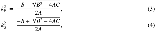 where
where
![Mathematical equation: \begin{eqnarray} \label{kdisper} A&=&c_{\rm s}^2\,v_{\rm A}^2,\\ B&=&-\left[\left(c_{\rm s}^2+v_{\rm A}^2\right)\omega^2-c_{\rm s}^2\,v_{\rm A}^2\,k_x^2 \right],\\ C&=&\omega^2\left[\omega^2-k_x^2\left(c_{\rm s}^2+v_{\rm A}^2\right)\right]. \end{eqnarray}](/articles/aa/full_html/2011/03/aa15862-10/aa15862-10-eq17.png) These
wavenumbers are associated to the same frequency ω and same
kx, and can be approximated, using the small
plasma-β assumption, by (e.g., Oliver
et al. 1992)
These
wavenumbers are associated to the same frequency ω and same
kx, and can be approximated, using the small
plasma-β assumption, by (e.g., Oliver
et al. 1992) 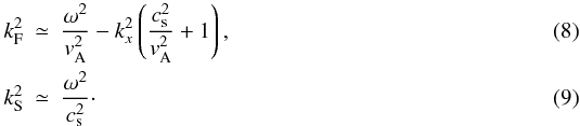 These
approximations will turn out to be useful in the following sections. According to Eq. (8) the fast wavenumber may become purely
imaginary for a certain choice of the parameters, indicating that the wave is evanescent.
Hereafter, we restrict our analysis to propagating waves.
These
approximations will turn out to be useful in the following sections. According to Eq. (8) the fast wavenumber may become purely
imaginary for a certain choice of the parameters, indicating that the wave is evanescent.
Hereafter, we restrict our analysis to propagating waves.
It can be seen from the linearised MHD equations that the velocity polarisation for fast
and slow modes is given by the following expression 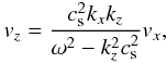 (10)where
kz is either kF
or kS. If we change the direction of propagation along the
field, kz changes to
− kz and the polarisation also changes
sign. In our configuration and in the regime that we are interested
(vA > cs), since
kF < kS, fast modes are
characterised by long wavelengths and by
vx > vz,
while slow modes have short wavelengths and
vx < vz.
The slow modes have a stronger compression since the wavelength is short in comparison with
the fast modes.
(10)where
kz is either kF
or kS. If we change the direction of propagation along the
field, kz changes to
− kz and the polarisation also changes
sign. In our configuration and in the regime that we are interested
(vA > cs), since
kF < kS, fast modes are
characterised by long wavelengths and by
vx > vz,
while slow modes have short wavelengths and
vx < vz.
The slow modes have a stronger compression since the wavelength is short in comparison with
the fast modes.
3. Propagating waves: the reflection problem
3.1. Fast MHD wave reflection
We consider that the most elementary problem shows the process of mode coupling due to
boundary conditions. A fast MHD wave travels downwards (in the negative
z-direction) and represents an incoming wave. This wave interacts with
the photosphere (located at z = 0, where line-tying conditions are
applied) and reflects (now travelling upwards). The amplitude of the fast incoming wave is
FI, while the amplitude of the reflected fast wave is
FR. To satisfy the boundary conditions, a slow MHD wave,
also moving upwards, must be generated at z = 0. The excited slow mode
has an amplitude SG. It is easy to write the velocity
components using the polarisation of fast and slow waves, given by Eq. (10), and the proper sign of the longitudinal
wavenumber, 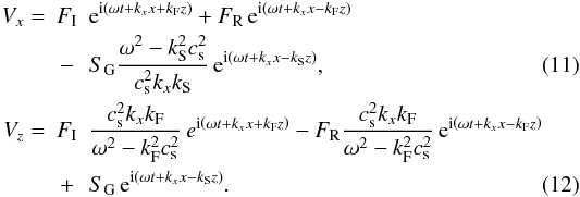 Now
boundary conditions are imposed at z = 0, representing the location of
the photosphere. We use line-tying conditions, i.e.,
Vx(z = 0) = Vz(z = 0) = 0.
According to Eqs. (11) and (12), the following conditions must be
satisfied,
Now
boundary conditions are imposed at z = 0, representing the location of
the photosphere. We use line-tying conditions, i.e.,
Vx(z = 0) = Vz(z = 0) = 0.
According to Eqs. (11) and (12), the following conditions must be
satisfied, 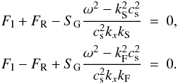 (13)The
solution in terms of the amplitude of the incoming wave (which is an arbitrary parameter)
is
(13)The
solution in terms of the amplitude of the incoming wave (which is an arbitrary parameter)
is 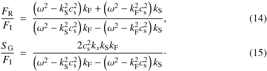 The
coefficients depend on ω, kx
(same for the three waves) and on longitudinal wavenumbers, kF
and kS, which can also be expressed in terms of
ω, kx by using Eqs. (3) and (4).
The
coefficients depend on ω, kx
(same for the three waves) and on longitudinal wavenumbers, kF
and kS, which can also be expressed in terms of
ω, kx by using Eqs. (3) and (4).
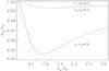 |
Fig. 1 Amplitude of reflected fast mode given by Eq. (14) as a function of the horizontal wavenumber for three different values of the sound speed. |
When there is no coupling between fast and slow modes (i.e., when
kx = 0) we find that
|FR/FI| = 1 because
 , while
SG/FI = 0. There is thus a
complete reflection of the incoming fast mode, while the slow mode is absent. When there
is coupling, the reflection coefficient for the slow mode is always different from zero,
meaning that the incoming fast MHD wave inevitably generates a slow mode at the boundary.
In Fig. 1 the reflection coefficient of the fast
wave, i.e., FR/FI, is plotted as
a function of kx for different values of the
sound speed. The coefficient is close to unity for values of low sound speed in comparison
with the Alfvén speed, meaning that reflection is almost total. However, for relatively
high values of cs/vA the curves
clearly show a minimum indicating that the reflection of the fast wave is less efficient.
, while
SG/FI = 0. There is thus a
complete reflection of the incoming fast mode, while the slow mode is absent. When there
is coupling, the reflection coefficient for the slow mode is always different from zero,
meaning that the incoming fast MHD wave inevitably generates a slow mode at the boundary.
In Fig. 1 the reflection coefficient of the fast
wave, i.e., FR/FI, is plotted as
a function of kx for different values of the
sound speed. The coefficient is close to unity for values of low sound speed in comparison
with the Alfvén speed, meaning that reflection is almost total. However, for relatively
high values of cs/vA the curves
clearly show a minimum indicating that the reflection of the fast wave is less efficient.
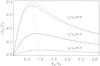 |
Fig. 2 Amplitude of the generated slow mode given by Eq. (15) as a function of the horizontal wavenumber for three different values of the sound speed. The dashed line represents the approximation given by Eq. (18) while the dotted line shows the position of the maxima according to Eqs. (19) and (20). |
In Fig. 2 the reflection coefficient of the slow
wave, i.e., SG/FI, is plotted.
The behaviour of the reflected slow mode amplitude is basically the opposite of the
reflected fast wave. The curves show a maximum at the locations where the generation of
the slow mode is more efficient. Again the value at the maximum strongly depends on the
ratio of the sound speed to the Alfvén speed, and corresponds to a
kx which is very similar to
kF. The location of the maximum can be analytically
determined from Eq. (15), and when using
the approximation of the slow mode frequency,  ,
,  (16)Since
the frequency is fixed, we have from the approximate expressions (8)–(9) for
(16)Since
the frequency is fixed, we have from the approximate expressions (8)–(9) for  and
and
 the following
relation
the following
relation  (17)Inserting
this expression to Eq. (16), we find that
(17)Inserting
this expression to Eq. (16), we find that
 (18)This
is a good approximation of the slow mode reflection coefficient (see dashed line in
Fig. 2), at least for the case
cs ≪ vA. It is used to determine
the location of the maxima of the curves in Fig. 2.
When imposing that the derivative of Eq. (18) is equal to zero, it is found that the maximum corresponds to
(18)This
is a good approximation of the slow mode reflection coefficient (see dashed line in
Fig. 2), at least for the case
cs ≪ vA. It is used to determine
the location of the maxima of the curves in Fig. 2.
When imposing that the derivative of Eq. (18) is equal to zero, it is found that the maximum corresponds to  (19)and
the value of the reflection coefficient for this horizontal wavenumber is
(19)and
the value of the reflection coefficient for this horizontal wavenumber is  (20)The
location and value of the maximum is represented in Fig. 2. There is excellent agreement between the approximation and the location of
the maximum calculated using the original expression for the reflection coefficient of the
slow mode (Eq. (15)). From Eq. (20) we see that the maximum amplitude of the
generated slow wave depends only on the β of the plasma.
(20)The
location and value of the maximum is represented in Fig. 2. There is excellent agreement between the approximation and the location of
the maximum calculated using the original expression for the reflection coefficient of the
slow mode (Eq. (15)). From Eq. (20) we see that the maximum amplitude of the
generated slow wave depends only on the β of the plasma.
Once we know the coefficients, it is straightforward to calculate magnitudes of interest
such as the density perturbation of the slow reflected wave as a function of amplitude of
the incoming fast wave. As we discuss later, these magnitudes can be directly related to
real observations. From the continuity equation (see Appendix A), the density perturbation for the slow mode is  (21)Using
again the fact that and Eq. (20) we find
(21)Using
again the fact that and Eq. (20) we find  (22)This
equation relates the maximum density perturbation associated to the generated slow mode
with the velocity amplitude of the incident fast wave.
(22)This
equation relates the maximum density perturbation associated to the generated slow mode
with the velocity amplitude of the incident fast wave.
3.2. The time-dependent problem
The time-dependent problem is numerically solved to demonstrate the mode coupling described in the previous section. The temporal evolution of the waves and specially their interaction with the boundaries provides a clear picture of the coupling and complements the analytical results.
In this numerical experiment a pulse in the
vx component is generated at
t = 0. This pulse has the following form 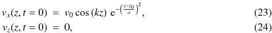 and
the rest of the perturbed variables are set to zero. This particular profile has the
property that represents a localised wave packet but with a rather well-defined wavelength
(basically given by λ = 2π/k). To
show the interaction of the fast mode with a single boundary, rigid conditions are applied
at z = 0
(vx(z = 0) = vz(z = 0) = 0)
while open conditions are imposed at z = L. The
linearised time-dependent MHD equations (see Appendix A) are numerically solved using standard finite differences techniques.
and
the rest of the perturbed variables are set to zero. This particular profile has the
property that represents a localised wave packet but with a rather well-defined wavelength
(basically given by λ = 2π/k). To
show the interaction of the fast mode with a single boundary, rigid conditions are applied
at z = 0
(vx(z = 0) = vz(z = 0) = 0)
while open conditions are imposed at z = L. The
linearised time-dependent MHD equations (see Appendix A) are numerically solved using standard finite differences techniques.
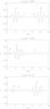 |
Fig. 3 Time evolution of the propagating disturbance given by Eqs. (23)–(24). The continuous line represents the vx component, while the vz component is plotted with a dotted line. Its amplitude has been multiplied by a factor 40 for visualisation purposes. Fast and slow modes travelling to the left are denoted as FI and SI, FI + and SI + move to the right, and SG is the generated wave at z = 0 (moving to the right). For this simulation z0/a = 5, ka = 2π/0.75, v0/vA = 1, kxa = 1.5 and cs/vA = 0.2. In this plot the time has been normalised to the characteristic time scale, τA = vA/a. |
The temporal evolution of the two velocity components is plotted in Fig. 3. The initial disturbance excites the fast mode, but also the slow mode, since the initial perturbation does not satisfy the velocity polarisation relation, given by Eq. (10). The excited fast and slow modes split in two identical modes propagating in opposite directions (top panel). The fast and slow waves travelling to the left are denoted as FI and SI, respectively, while FI + and SI + move to the right. Once the FI mode reaches the rigid boundary (z = 0), it gets reflected (see middle panel) with an amplitude FR and a slow mode is generated; i.e., the SG mode according to the notation introduced above. The slow wave packet has a typical wavelength much smaller than the fast wavelength (kF ≪ kS). At the other boundary (z = L), the fast mode FI + leaves the system owing to the transparent boundary conditions. At later times (bottom panel), the SG and SI modes, moving in opposite directions, start to superpose, while the FR and SI + , travelling in the same direction, also interfere.
The amplitudes of reflected fast and slow waves estimated from the time-dependent problem agree quite well with the calculations based on the analytical reflection coefficients given by Eqs. (14)–(15). These equations were derived for purely sinusoidal and monochromatic waves, but the initial packet is represented well by a dominant frequency (wavelength), and this is the reason it agrees with the analytical results.
3.3. Slow MHD wave reflection
Although we are mainly interested in the fast reflection problem, the slow mode
reflection problem is also studied for completeness. The difference with respect to the
fast MHD reflection problem is that reflection of the slow MHD mode at the boundary
generates a fast MHD mode. The velocity components for this problem are  The
following coefficients for the reflected slow mode and the generated fast mode are found
by applying rigid boundary conditions
The
following coefficients for the reflected slow mode and the generated fast mode are found
by applying rigid boundary conditions  It
is worth noting that the reflection coefficient of the slow mode is exactly the same as
the reflection coefficient of the fast mode given by Eq. (14).
It
is worth noting that the reflection coefficient of the slow mode is exactly the same as
the reflection coefficient of the fast mode given by Eq. (14).
4. Standing waves
Once we understand the reflection of a propagating fast and a propagating slow wave at a rigid boundary we extend our analysis to a more realistic physical situation, i.e., the standing fast wave problem that is commonly reported by TRACE.
There are several ways to study this problem, and the perturbation method is one of them. Under this approach, we know that for zero-β we have a pure standing fast wave with only a vx velocity component that satisfies the boundary conditions. When β is different from zero but small, a vz component is introduced, due to Eq. (10), and even worse, this component does not satisfy the boundary condition. To compensate, we have to add a slow wave perturbation to the system (with a dominant vz in comparison with vx), which combined with the vz of the fast, will satisfy the boundary conditions jointly. Now the vx introduced by the slow mode is irrelevant since it is higher order in β (which is assumed to be small).
Another way to analyse this problem is to solve the full-standing problem. This has already been done by Oliver et al. (1992) and Goedbloed & Halberstadt (1994), and it is based on the superposition of the fast reflection problem plus the slow reflection problem. The perturbation scheme and the full eigenmode problem give similar results, except where the solutions are completely mixed, i.e., when the slow mode component is not small in comparison with the fast component. This takes place around the “avoided crossings” in the dispersion diagram (see Oliver et al. 1992, for further details).
The advantage of the perturbation scheme is that we can still obtain simple approximations
for the velocity and density changes around the footpoints. Let us assume that an initial
disturbance mostly excites the standing pattern in the
vx component. This standing wave is
composed by the superposition of two identical propagating waves travelling in opposite
directions. We concentrate on the fundamental mode, having a maximum at
z = L/2 and a node of the velocity at the boundaries.
A propagating slow wave is induced by the reflection at the boundaries of the incident
propagating fast wave that forms part of the standing fast pattern. As a result, if the
transverse velocity amplitude of the standing fast wave at the loop apex is
V0, the amplitude of the incoming fast wave is
V0/2. The reflected fast wave will also have an amplitude of
V0/2 in our approximation. Once we know this amplitude, it
is easy to estimate the velocity or density fluctuations associated to the slow mode using
the results of the propagation problem. According to the analysis performed in the previous
section (see Eqs. (20) and (22)),  (29)and
 (30)These
very simple expressions give the order of the maximum velocity and density perturbations
associated to the slow reflected mode as a function of the transverse velocity amplitude at
the loop apex and the characteristic speeds of the configuration. When
cs ≪ vA the velocity perturbation
reduces to
(30)These
very simple expressions give the order of the maximum velocity and density perturbations
associated to the slow reflected mode as a function of the transverse velocity amplitude at
the loop apex and the characteristic speeds of the configuration. When
cs ≪ vA the velocity perturbation
reduces to  (31)while
the density perturbation is
(31)while
the density perturbation is  (32)It
is worth calculating the order of magnitude of velocity and density fluctuations around the
footpoint. Let us take typical values:
vA = 800 km s-1,
cs = 200 km s-1,
V0 = 80 km s-1. Thus, the velocity perturbation
according to Eq. (29) is
|vz|max ≃ 2.5 km s-1.
Using Eq. (30) we find that the density
fluctuation associated to the slow mode is
|ρ1/ρ|max ≃ 1.25%. These density
perturbations, although small, should be detectable with the current instruments. Obviously,
larger sound speeds or small Alfvén velocities would result in an increase in velocity and
density fluctuations.
(32)It
is worth calculating the order of magnitude of velocity and density fluctuations around the
footpoint. Let us take typical values:
vA = 800 km s-1,
cs = 200 km s-1,
V0 = 80 km s-1. Thus, the velocity perturbation
according to Eq. (29) is
|vz|max ≃ 2.5 km s-1.
Using Eq. (30) we find that the density
fluctuation associated to the slow mode is
|ρ1/ρ|max ≃ 1.25%. These density
perturbations, although small, should be detectable with the current instruments. Obviously,
larger sound speeds or small Alfvén velocities would result in an increase in velocity and
density fluctuations.
The previous estimations are based on the assumption that the excited slow modes do not have time to reach the opposite footpoint and reflect. If this is the case, the problem is more difficult since the slow modes interfere, and the velocity and density changes can be greater than those given by Eqs. (29)–(30). It is also important to notice that the density perturbation associated to the fast standing mode has the same profile as the velocity (the vx component), therefore the fast density perturbation is zero at the footpoints (and maximum at the apex). This explains why it is enough to consider only the density changes associated to the excited slow modes around the footpoints.
4.1. The time-dependent problem
Now the time-dependent problem is solved. The initial perturbation, representing the
excitation of a mainly fast standing wave, has the following profile, 
4.1.1. Rigid boundary conditions
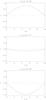 |
Fig. 4 Time evolution of the standing fast excitation given by Eqs. (33)–(34). The continuous line represents the vx component, while the vz component is plotted with a dotted line. Its amplitude has been multiplied by a factor 10 for visualisation purposes. For this simulation ka = π/10, v0/vA = 1, kxa = 1.5 and cs/vA = 0.2. |
Line-tying conditions are applied at the two loop footpoints. We choose the longitudinal wavenumber that excites the fundamental standing fast MHD mode, i.e., k = π/L. The results, represented in Fig. 4 manifest the generation of slow modes at the footpoints (top panel). The fast mode drives slow modes, which move in the direction of the loop apex, located at z = L/2 (see middle panel). At a certain time (when t ≃ L/2cs) the interference between the opposite propagating slow waves is produced. Since the two slow waves are identical but travelling in opposite directions a quasi-standing pattern is visible (see the profile of vz around z = 5a in the bottom panel). Eventually, slow modes reach the opposite footpoint and get reflected. Under such conditions the inverted process takes place; i.e., the slow mode generates a fast mode. Nevertheless, this problem would take us too far beyond the scope of this work. However, it is worth noting that depending on the equilibrium and wave parameters the generated slow modes might match the frequency of a standing slow eigenmode of the loop. This means that since the slow mode is driven by the fast standing mode, the frequencies of the slow standing and fast standing waves will be basically the same and the modes will have a highly mixed nature. This takes place around the “avoided crossings” in the dispersion diagram.
4.1.2. Sharp photosphere-corona transition
From the previous results we might think that the generation of slow modes takes place
only when rigid boundary conditions are imposed. To address this question, instead of
line-tying conditions, a density transition between the corona and the photosphere is
considered. As density profile we use the following idealised model, 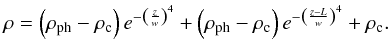 (35)Parameter
w measures the width of the transition between the photosphere, with
density ρph, and corona, with density
ρc. The density contrast is set to
ρph/ρc = 108.
Non-reflecting conditions are imposed at the boundaries, now placed below the
photosphere. The details of the model used to represent the transition
photosphere-corona are not important since our focus is on the generated slow modes. The
equilibrium gas pressure is set to the same constant value in the corona and photosphere
to have magnetohydrostatic equilibrium.
(35)Parameter
w measures the width of the transition between the photosphere, with
density ρph, and corona, with density
ρc. The density contrast is set to
ρph/ρc = 108.
Non-reflecting conditions are imposed at the boundaries, now placed below the
photosphere. The details of the model used to represent the transition
photosphere-corona are not important since our focus is on the generated slow modes. The
equilibrium gas pressure is set to the same constant value in the corona and photosphere
to have magnetohydrostatic equilibrium.
 |
Fig. 5 Time evolution of the standing fast excitation given by Eqs. (33)–(34) with the density model given by Eq. (35). The continuous line represents the vx component, while the vz component is plotted with a dotted line (its amplitude has been multiplied by a factor 10 for visualisation purposes). The vertical dashed lines represent the locations of the transition between the corona and photosphere. For this simulation ka = π/9, v0/vA = 1, kxa = 1.5, cs/vA = 0.2, ρph/ρc = 108, w/a = 0.25. |
The results of the time-dependent simulation are plotted in Fig. 5. There are some differences with respect to the behaviour found for the perfectly reflecting boundaries. For example, the system now allows the energy to escape through the photosphere; i.e., there is a transmitted fast (and slow wave). This means that the energy can leak through the photosphere but this is not visible in Fig. 5 because the amplitude is very small. Nevertheless, the primary result here is that a similar slow-mode generation in comparison with the case of reflecting boundaries is produced in the coronal part (compare Figs. 4 and 5). The results are qualitatively similar, so, the overall conclusion is that nonuniformity causes the coupling between fast and slow modes in a similar way to line-tying conditions.
5. Link with observations
It is interesting to look for signatures of the mode coupling studied in this work in the observations. Recently, Verwichte et al. (2010) have reported from combined observations with TRACE and EIT/SoHO, intensity fluctuations at one loop footpoint with basically the same period, around 40 min, as the fast transverse oscillation of the loop. This long periodicity indicates that the origin of these density oscillations is most probably not photospheric. Verwichte et al. (2010) suggest that the intensity oscillations are due to variations in the line-of-sight column depth produced by the changes in the loop inclination as it oscillates with the transverse kink mode. This would explain the coincidence in periods and also in the damping times.
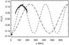 |
Fig. 6 Relative profile of intensity variations seen in a transversely oscillating loop studied by Verwichte et al. (2010) using TRACE as a function of distance along the loop. The solid circle is the measurement of the intensity variation at the loop foot point. The long-dashed and dashed curves are functions –0.13sin(3π/L) and –0.13sin(5π/L), respectively, representing a possible third or fifth standing harmonic of the slow mode. |
According to our study, an alternative explanation for the intensity variations reported by Verwichte et al. (2010) is done in terms of the coupling between fast and slow waves due to the line-tying conditions. The similarity of the periods of the transverse mode and the intensity fluctuations is explained by our model where the excited slow wave, as well as the corresponding intensity oscillation, has the same periodicity as the transverse loop motion. Verwichte et al. (2010) show intensity variations associated with a transverse oscillation in a large loop of 690 ± 60 Mm length. The oscillation, which is a horizontally polarised fundamental kink mode, has a period of P = 2418 ± 5 s. Therefore, the phase speed is equal to vph = 580 ± 50 km s-1. For a thin loop in the long wavelength limit, this phase speed tends to the kink speed, ck, of a cylindrical tube. If the intensity oscillation is associated with a slow magnetoacoustic mode with the same periodicity as the kink mode, then its wavelength is equal to λs = csP = (csP/vph)2L. For a temperature between 0.9 and 1.8 MK, the coronal sound speed is in the range 144–198 km s-1. Hence, λs = (0.30 ± 0.07) 2L. For a standing mode, this translates into a wavenumber n = vph/cs = 2L/λs = 3.3 ± 1.0. The EIT observations suggests that the intensity variations at the two foot points of the loop oscillate in anti-phase. If standing, the mode should be an odd harmonic. Figure 6 shows the relative profile of intensity variations as a function of loop distance. The relative intensity has an amplitude of approximately 13%, which translates into a density perturbation with an amplitude, | ρ1/ρ | max = 6.5%. However, it is clear that a third or fifth harmonic could fit the observed intensity variation if we consider that the slow mode is most likely still evolving towards a standing wave pattern. We measured the full intensity profile as a function of distance along the loop using EIT. Nevertheless, this has large uncertainties attached to it because of the lack of resolution and line-of-sight confusion. Also, the loop may be longitudinally structured in temperature. The EIT measurement hints at the presence of a fifth harmonic. Verwichte et al. (2010) show that the displacement amplitude, ξ0, can be modelled by a ten degree inclination of the loop. As the loop has a height of 236 Mm this means that ξ0 = 41 Mm. Hence, the velocity amplitude V0 = ξ0ω = 106 km s-1. Using Eq. (30) and the estimated value for the Alfvén speed, vA = 410 ± 40 km s-1, we find |ρ1/ρ| max = 5 ± 3%. This is consistent with the observed density amplitude (around 6.5%).
In another work, Verwichte et al. (2009) also report intensity oscillations associated with a kink mode seen by EUV onboard STEREO and interpreted these as resulting from variations in the line-of-sight column depth owing to the loop showing a varying aspect to the observer. The measured relative density amplitude is 2.5% and is located around to loop top. Can this observation be explained by a slow mode instead? In that observation, the key parameters that were measured are L = 340 ± 15 Mm, vph = 1100 ± 100 km s-1, V0 = 35 ± 9 km s-1, and vA = 800 ± 100 km s-1. For the peak temperature of the EUV 171 Å bandpass of 0.9 MK, cs = 144 km s-1. The slow mode would have a wavenumber n = 7 ± 1 (in the case of a standing mode), corresponding to a wavelength of about λs = 90 ± 10 Mm. Again, using Eq. (30), we calculate |ρ1/ρ| max = 0.4%, which is negligibly small. Therefore, for this observation, the slow mode is not able to explain the observed intensity variations. The main difference with respect to the case studied by Verwichte et al. (2010) is that the density perturbations are located around the loop top instead of the loop footpoints.
6. Discussion and conclusions
In this work we have investigated the possible effects of linear coupling between fast and slow modes that takes place due to the reflection at the photosphere. By solving the reflection problem, we have shown that the transverse motion of the loop produces slow MHD waves as long as the fast wave is obliquely incident on the boundary. These slow waves are manifested as propagating density fluctuations with the same frequency as the standing transverse mode and are generated at the loop footpoints. The wavelength of these slow modes is basically given by ks ≃ ω/cs, and since vA > cs their wavelength is smaller than that of the corresponding fast standing transverse mode. Moreover, we used the reflection coefficient of the slow mode to derive simple analytical expressions that relate the transverse displacement at the loop top with the amplitude of the density fluctuations produced at the footpoints. The coupling between fast and slow is proportional to the plasma-β, indicating that it will be weak under coronal conditions. However, it is proportional to the amplitude of the oscillation of the fast mode, which can be large in some cases, and close to the footpoints, i.e., close to the photosphere, the ratio between the sound and Alfvén speeds can increase. Ideally, from the properties of the reflected slow modes, we could have indirect information about the real line-tying conditions in coronal loops and realistic values of the sound speed near the footpoints.
The generated slow waves can eventually form a standing pattern along the loop. Thus, mode coupling might provide an excitation mechanism of standing slow modes, different from the driven photospheric origin usually emphasised in the literature. However, since the sound speed is assumed to be slower than the Alfvén speed, the time required for the slow mode to travel along the loop and reflect at the footpoint is much longer than that of the fast MHD mode. This means that slow-standing modes will need much more time than fast-standing modes to build up. Nevertheless, if the wavelength of the slow modes is very short they might be damped by thermal conduction before the standing wave is formed.
It has been shown that, in the observations analysed by Verwichte et al. (2010), there are possible fingerprints of the coupling between fast and slow modes owing to line-tying, providing an alternative explanation to the effects of integration along the line of sight proposed by these authors. However, in the observations studied by Verwichte et al. (2009), the mechanism is unable to explain the intensity oscillations. One of the reasons might be that the density changes observed in this event are reported around the loop apex, while the estimations are based on propagating waves around the footpoints. In the case of the standing pattern, the density fluctuations can be much larger. Further analysis of other observations will test the linear coupling as an operative mechanism in coronal loops.
It is worth mentioning that the mode coupling discussed in the work is a purely linear effect. It is unrelated to the nonlinear coupling between fast and slow modes due to the ponderomotive force (see Hollweg 1971; Rankin et al. 1994; Terradas & Ofman 2004) or to the parametric coupling studied by Zaqarashvili et al. (2002, 2005). It is also different from the mode conversion that takes place when cs = vA. Line-tying boundary conditions are the responsible ingredients of the coupling, but we have shown that they are not the only way for fast and slow waves to couple. A sharp transition between the corona and the photosphere produces the generation of slow modes, i.e., a change in the properties of the medium, for example the transition region, leads inevitably to the coupling.
Our theoretical model is based on a Cartesian geometry without a density enhancement representing a loop. For this reason, it is necessary to improve the model by including a slab or a cylinder that mimics the effect of a dense magnetic tube. This will complicate the mathematical problem of the reflection at the boundary, and it might be difficult to derive simple analytical expressions. For example, in a cylindrical model, the eigenfunctions of the slow and fast MHD waves have different radial dependencies and might share the same azimuthal wavenumber (basically playing the role of kx in the present work). This issue will be addressed in a future study.
Acknowledgments
J.T. acknowledges the Universitat de les Illes Balears for a postdoctoral position and the financial support received from the Spanish MICINN and FEDER funds (AYA2006-07637). J.T. thanks Ramón Oliver and Roberto Soler for useful comments and suggestions. J.A. is supported by an International Outgoing Marie Curie Fellowship within the 7th European Community Framework Programme. J.A. also acknowledges support by the Fund for Scientific Research – Flanders. E.V. acknowledges financial support from the UK Engineering and Physical Sciences Research Council (EPSRC) Science and Innovation award.
References
- Aschwanden, M. J., Fletcher, L., Schrijver, C. J., & Alexander, D. 1999, ApJ, 520, 880 [NASA ADS] [CrossRef] [Google Scholar]
- Aschwanden, M. J., de Pontieu, B., Schrijver, C. J., & Title, A. M. 2002, Sol. Phys., 206, 99 [NASA ADS] [CrossRef] [Google Scholar]
- De Moortel, I. 2009, Space Sci. Rev., 149, 65 [NASA ADS] [CrossRef] [Google Scholar]
- Erdélyi, R., & Taroyan, Y. 2008, A&A, 489, L49 [NASA ADS] [CrossRef] [EDP Sciences] [Google Scholar]
- Goedbloed, J. P., & Halberstadt, G. 1994, A&A, 286, 275 [NASA ADS] [Google Scholar]
- Hollweg, J. V. 1971, J. Geophys. Res., 76, 5155 [NASA ADS] [CrossRef] [Google Scholar]
- Mariska, J. T. 2005, ApJ, 620, L67 [NASA ADS] [CrossRef] [Google Scholar]
- Mariska, J. T. 2006, ApJ, 639, 484 [NASA ADS] [CrossRef] [Google Scholar]
- Nakariakov, V. M., Ofman, L., Deluca, E. E., Roberts, B., & Davila, J. M. 1999, Science, 285, 862 [NASA ADS] [CrossRef] [PubMed] [Google Scholar]
- Oliver, R., Ballester, J. L., Hood, A. W., & Priest, E. R. 1992, ApJ, 400, 369 [NASA ADS] [CrossRef] [Google Scholar]
- Rankin, R., Frycz, P., Tikhonchuk, V. T., & Samson, J. C. 1994, J. Geophys. Res., 99, 21291 [NASA ADS] [CrossRef] [Google Scholar]
- Schrijver, C. J., & Brown, D. S. 2000, ApJ, 537, L69 [NASA ADS] [CrossRef] [Google Scholar]
- Schrijver, C. J., Aschwanden, M. J., & Title, A. M. 2002, Sol. Phys., 206, 69 [NASA ADS] [CrossRef] [Google Scholar]
- Stein, R. F. 1971, ApJS, 22, 419 [NASA ADS] [CrossRef] [Google Scholar]
- Terradas, J., & Ofman, L. 2004, ApJ, 610, 523 [NASA ADS] [CrossRef] [Google Scholar]
- Vasquez, B. J. 1990, ApJ, 356, 693 [NASA ADS] [CrossRef] [Google Scholar]
- Verwichte, E., Aschwanden, M. J., Van Doorsselaere, T., Foullon, C., & Nakariakov, V. M. 2009, ApJ, 698, 397 [NASA ADS] [CrossRef] [Google Scholar]
- Verwichte, E., Foullon, C., & Van Doorsselaere, T. 2010, ApJ, 717, 458 [NASA ADS] [CrossRef] [Google Scholar]
- Wang, T., Innes, D. E., & Qiu, J. 2007, ApJ, 656, 598 [NASA ADS] [CrossRef] [Google Scholar]
- Wang, T. J., Solanki, S. K., Curdt, W., et al. 2003a, A&A, 406, 1105 [NASA ADS] [CrossRef] [EDP Sciences] [Google Scholar]
- Wang, T. J., Solanki, S. K., Innes, D. E., Curdt, W., & Marsch, E. 2003b, A&A, 402, L17 [NASA ADS] [CrossRef] [EDP Sciences] [Google Scholar]
- Zaqarashvili, T. V., Oliver, R., & Ballester, J. L. 2002, ApJ, 569, 519 [NASA ADS] [CrossRef] [Google Scholar]
- Zaqarashvili, T. V., Oliver, R., & Ballester, J. L. 2005, A&A, 433, 357 [NASA ADS] [CrossRef] [EDP Sciences] [Google Scholar]
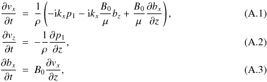
Appendix A:
We use the linearised MHD equations of the momentum, induction, energy, and continuity
equation. Assuming Fourier analysis in the x − direction we have
 \newpage
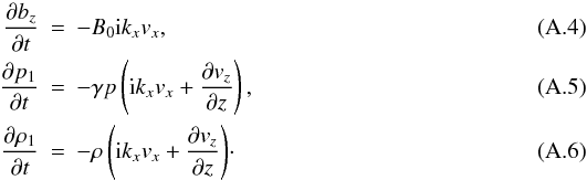 In
these equations B0 is the equilibrium magnetic field and
ρ and p the equilibrium density and gas pressure,
respectively. The rest of the variables correspond to the perturbed magnitudes. To
eliminate the imaginary complex numbers we simply define
In
these equations B0 is the equilibrium magnetic field and
ρ and p the equilibrium density and gas pressure,
respectively. The rest of the variables correspond to the perturbed magnitudes. To
eliminate the imaginary complex numbers we simply define
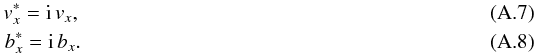 With
this transformation the time-dependent equations are solved using standard numerical
techniques.
With
this transformation the time-dependent equations are solved using standard numerical
techniques.
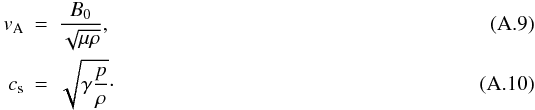
The dispersion relation, given by Eq. (1),
is easily derived assuming in the previous equations a temporal dependence of the form
eiωt and a spatial dependence with the
z-coordinate of the form
eikzz. We
used the following standard definitions for the Alfvén and sound speeds,
All Figures
|
Fig. 1 Amplitude of reflected fast mode given by Eq. (14) as a function of the horizontal wavenumber for three different values of the sound speed. |
| In the text | |
|
Fig. 2 Amplitude of the generated slow mode given by Eq. (15) as a function of the horizontal wavenumber for three different values of the sound speed. The dashed line represents the approximation given by Eq. (18) while the dotted line shows the position of the maxima according to Eqs. (19) and (20). |
| In the text | |
|
Fig. 3 Time evolution of the propagating disturbance given by Eqs. (23)–(24). The continuous line represents the vx component, while the vz component is plotted with a dotted line. Its amplitude has been multiplied by a factor 40 for visualisation purposes. Fast and slow modes travelling to the left are denoted as FI and SI, FI + and SI + move to the right, and SG is the generated wave at z = 0 (moving to the right). For this simulation z0/a = 5, ka = 2π/0.75, v0/vA = 1, kxa = 1.5 and cs/vA = 0.2. In this plot the time has been normalised to the characteristic time scale, τA = vA/a. |
| In the text | |
|
Fig. 4 Time evolution of the standing fast excitation given by Eqs. (33)–(34). The continuous line represents the vx component, while the vz component is plotted with a dotted line. Its amplitude has been multiplied by a factor 10 for visualisation purposes. For this simulation ka = π/10, v0/vA = 1, kxa = 1.5 and cs/vA = 0.2. |
| In the text | |
|
Fig. 5 Time evolution of the standing fast excitation given by Eqs. (33)–(34) with the density model given by Eq. (35). The continuous line represents the vx component, while the vz component is plotted with a dotted line (its amplitude has been multiplied by a factor 10 for visualisation purposes). The vertical dashed lines represent the locations of the transition between the corona and photosphere. For this simulation ka = π/9, v0/vA = 1, kxa = 1.5, cs/vA = 0.2, ρph/ρc = 108, w/a = 0.25. |
| In the text | |
|
Fig. 6 Relative profile of intensity variations seen in a transversely oscillating loop studied by Verwichte et al. (2010) using TRACE as a function of distance along the loop. The solid circle is the measurement of the intensity variation at the loop foot point. The long-dashed and dashed curves are functions –0.13sin(3π/L) and –0.13sin(5π/L), respectively, representing a possible third or fifth standing harmonic of the slow mode. |
| In the text | |
Current usage metrics show cumulative count of Article Views (full-text article views including HTML views, PDF and ePub downloads, according to the available data) and Abstracts Views on Vision4Press platform.
Data correspond to usage on the plateform after 2015. The current usage metrics is available 48-96 hours after online publication and is updated daily on week days.
Initial download of the metrics may take a while.