| Issue |
A&A
Volume 527, March 2011
|
|
|---|---|---|
| Article Number | A7 | |
| Number of page(s) | 5 | |
| Section | Stellar structure and evolution | |
| DOI | https://doi.org/10.1051/0004-6361/201015737 | |
| Published online | 18 January 2011 | |
Finding a 24-day orbital period for the X-ray binary 1A 1118-616
1
Institut für Astronomie und Astrophysik, Abteilung Astronomie, Universität
Tübingen (IAAT),
Sand 1,
72076
Tübingen,
Germany
e-mail: staubert@astro.uni-tuebingen.de
2
NASA-Goddard Space Flight Center, Astrophysics Science Division,
Code 661,
Greenbelt, MD
20771,
USA
3
Center for Space Science and Technology (CRESST), University of
Maryland Baltimore County, 1000
Hilltop Circle, Baltimore, MD
21250,
USA
4
Dr. Karl Remeis-Sternwarte and Erlangen Center for Astroparticle
Physics, Universität Erlangen-Nürnberg, Sternwartstr. 7, 96049
Bamberg,
Germany
5
Center for Astrophysics and Space Sciences (CASS), University of
California San Diego, La
Jolla, CA
92093-0424,
USA
Received: 10 September 2010
Accepted: 2 November 2010
We report the first determination of the binary period and orbital ephemeris of the Be X-ray binary containing the pulsar 1A 1118-616 (35 years after the discovery of the source). The orbital period is found to be Porb = 24.0 ± 0.4days. The source was observed by RXTE during its last large X-ray outburst in January 2009, which peaked at MJD 54845.4, by taking short observations every few days, covering an elapsed time comparable to the orbital period. Using the phase connection technique, pulse arrival time delays could be measured and an orbital solution determined. The data are consistent with a circular orbit and the time of 90 degrees longitude was found to be Tπ/2 = MJD 54845.37(10), which is coincident with that of the peak X-ray flux.
Key words: binaries: general / stars: neutron / X-rays: general / X-rays: binaries / X-rays: individuals: 1A 1118-616 / ephemerides
© ESO, 2011
1. Introduction
The X-ray transient 1A 1118−61 was discovered during an outburst in 1974 by the Ariel-5 satellite in the 1.5–30keV range (Eyles et al. 1975). The modulation with a period of 6.75min found in the data used by Ives et al. (1975) was initially interpreted as the orbital period of two compact objects. Fabian et al. (1975) then suggested that the observed period may be due to a slowly spinning accreting neutron star in a binary system. The optical counterpart was identified as the Be-star He 3-640/Wray 793 by Chevalier & Ilovaisky (1975) and classified as an O9.5IV-Ve star with strong Balmer emission lines and an extended envelope by Janot-Pacheco et al. (1981). The distance was estimated to be 5 ± 2kpc (Janot-Pacheco et al. 1981). The classification and distance was confirmed by Coe & Payne (1985) using UV observations of the source.
 |
Fig.1 The light curve of the outburst of 1A 1118-616 as observed by RXTE/PCA (4–40keV) in January 2009. The time resolution is 16s. The continuous curve is the daily light curve as seen by RXTE/ASM (scaled to the PCA count rate and smoothed by taking the running mean of five consecutive days). |
A second strong X-ray outburst occurred in January 1992, which was observed by CGRO/BATSE (Coe et al. 1994). The measured peak flux was ~150 mCrab for the 20–100keV energy range, similar to that of the 1974 outburst. This outburst was followed by enhanced X-ray activity for ~60 days, with two flare-like events about ~25 d and ~49 d after the peak of the outburst (see Coe et al. 1994, Fig. 1). Pulsations with ~406.5 s were detected up to 100keV and the pulse profile showed a single broad peak, close to a sinusoidal modulation with little change with photon energy. A spin-up with a rate of 0.016s/day was observed during the decay of the outburst. Multi-wavelength observations revealed a strong correlation between the Hα equivalent width and the X-ray flux. This led Coe et al. (1994) to conclude that expansion of the circumstellar disk of the optical companion is mainly responsible for the increased X-ray activity, including a large outburst if there is enough matter in the system. This conclusion is supported by the pulsations from the source also being detected in quiescence (Rutledge et al. 2007).
The source remained quiescent until January 4, 2009 when a third outburst was detected by Swift (Mangano et al. 2009; Mangano 2009). Pulsations with a period of 407.68 ± 0.02s were reported by Mangano (2009). The complete outburst was regularly monitored by RXTE. INTEGRAL observed the source after the main outburst (Leyder et al. 2009). Suzaku observed 1A 1118 − 61 twice, once during the peak of the outburst and also ~20 days later when the flux returned to its previous level. Doroshenko et al. (2010) analyzed RXTE/PCA data of the most recent outburst with emphasis on spectral analysis, detecting a cyclotron resonant scattering feature (CRSF) at ~55 keV.
In this paper, we report on an in-depth timing analysis of RXTE/PCA data over the entire outburst in January 2009, and the discovery of an orbital period of 24.0d. This solution is supported by the timing of the three large X-ray outbursts seen in history and by the analysis of pulse arrival times of the January 1992 BATSE observations.
2. Observations
We used two data sets. First, and most importantly, we analyzed data obtained by RXTE/PCA during a 27-day monitoring of 1A 1118-616, which started on January 7, 2009, covering the complete outburst. The resulting light curve (4–40keV) is shown in Fig. 1. The source flux peaked on January 14 and decayed over ~15 days. The data structure is defined by the orbits of the RXTE satellite, with 29 RXTE pointings of a typical duration of around one hour. A total exposure of 87ks was obtained. The PCA data were all taken in event mode (“Good Xenon”), providing arrival times for individual events. The data were reduced using HEASOFT version 6.8.
A second data set consists of pulse profiles generated from archival data of the observation of the January 1992 outburst by CGRO/BATSE, covering about 12days.
 |
Fig.2 An example of a pulse profile (with 32 phase bins) of 1A 1118-616 as observed in ~2.5 ks by RXTE/PCA (normalized to a mean flux of 1.0), corresponding to the folding of 6 pulses with a pulse period of ~407.7 s. The center of the observing time is MJD 54844.375. The profile is repeated such that two phases are shown.This profile was used as a template in measuring relative phase shifts of profiles from other integration intervals and the corresponding pulse arrival times. |
3. Timing analysis of pulse arrival times
3.1. RXTE/PCA – 2009
Some timing analysis of the RXTE data was performed earlier by Doroshenko et al. (2010), who determined the pulse period and an initial value of its derivative but failed to identify the orbital modulation. Here, a more rigorous analysis is performed, which begins in a similar way by selecting 19 integration intervals of the 29 pointings according to the time structure of the individual satellite pointings (Fig. 1). These integration intervals ranged from ~1500 s to ~15000 s, corresponding to between four and 38 pulses. Nineteen pulse profiles (with 32 phase bins) were then constructed by epoch-folding barycenter-corrected event times (since the Earth is always moving with respect to the source, the event arrival times are referenced to the center of the solar system). Figure 2 shows one of these pulse profiles produced by accumulating six pulses (centered at MJD 54844.375). Using this profile, the pulse arrival times (in MJD) for the other profiles were determined by template fitting. The uncertainties of these arrival times are of the order of 10s (~2.5% of the pulse period).
For the case of no binary modulation and non-zero first and second derivatives of the pulse period, the expected arrival times as a function of pulse number n are given by (see, e.g., Kelley et al. 1980; Nagase 1989; Staubert et al. 2009)  (1)With the given accuracy, it was possible to phase-connect the 19 pulse arrival times and determine values for the pulse period and its first derivative by applying a quadratic fit in n. The sond derivative
  was not constrained and set to zero. In this fit, significant systematic residuals remained with a sine-like shape and an amplitude of several tens of seconds, indicative of pulse arrival-time delays due to orbital motion. Adding the additional term
 ![\begin{equation} +~a\sin~i \times \cos[2\pi~(t-T_{\pi/2})/P_{\rm orb}] \label{cos} \end{equation}](/articles/aa/full_html/2011/03/aa15737-10/aa15737-10-eq11.png) (2)yielded an acceptable fit as expected for a circular binary orbit, asini being the projected radius of the orbit in light-seconds, and Tπ/2( = T90) in MJD being the time at which the mean orbital longitude of the neutron star is 90°, corresponding to the maximum delay in pulse arrival time. We found that asini ~ 55 light-s, Porb ~ 24 d, T90 MJD ~ 54845, Ppulse ~ 407.7 s, and Ṗs ~ −1.9 × 10⁻⁷ss-1.
(2)yielded an acceptable fit as expected for a circular binary orbit, asini being the projected radius of the orbit in light-seconds, and Tπ/2( = T90) in MJD being the time at which the mean orbital longitude of the neutron star is 90°, corresponding to the maximum delay in pulse arrival time. We found that asini ~ 55 light-s, Porb ~ 24 d, T90 MJD ~ 54845, Ppulse ~ 407.7 s, and Ṗs ~ −1.9 × 10⁻⁷ss-1.
 |
Fig.3 An example light curve with 16s resolution of one continuous observation by RXTE/PCA in the 4–40keV interval, together with the best-fit cosine function. |
We then realized that by using the original light curve, a sample of which is shown in Fig. 3, we were able to determine the pulse arrival times more accurately, when fitted piecewise with a cosine function (keeping the pulse period fixed at the previously found best-fit values, and leaving the mean flux, the amplitude, and the zero phase as free parameters). The same 19 integration intervals as before were used. The phase connection analysis of the pulse arrival times determined in this way then leads to the orbital elements and pulse period information summarized in Table 1. The pulse delay times and the residuals against the expected delays for the best-fit circular orbit is shown in Fig. 4. The χ2 of this best fit was 21.0 for 15dof (degrees of freedom).
In finding this solution, we assumed a vanishing eccentricity and a fixed value of 24.0d for the orbital period. When the orbital period was left as a free parameter, we found that Porb = 24.0 ± 0.4d. This uncertainty is expected to be large since our observations cover only 27days, little more than one orbital cycle.
Orbital elements, Ppulse and Ṗpulse of 1A 1118-616.
Finally, we attempted a proper orbital solution with the eccentricity ϵ and the longitude of periastron passage Ω included as free parameters by solving Kepler’s equation. The data do allow one to define a pair of parameters with reasonably constrained uncertainties of ϵ = 0.10 ± 0.02 and Ω = (310 ± 30)°. However, we consider the evidence of a non-zero eccentricity as marginal. By introducing these two additional free parameters, the χ2 was reduced from 21.0 (15 d.o.f.) to 16.4 for (13 d.o.f.). An F-test yielded a rather large probability of ~22% for the improvement to have occured by chance. Furthermore, no systematic uncertainties of any kind were considered.
We note that the values for the pulse period and its derivative given in Table 1 differ from those stated by Doroshenko et al. (2010) because of the missing orbital corrections in the earlier analysis.
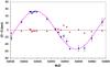 |
Fig.4 Delays of the pulse arrival times in 1A 1118-616 for the outburst of January 2009 as observed by RXTE/PCA and best-fit sine curve for circular orbital motion with a period of 24.0d. The dots around zero are the residuals to the best-fit solution. |
 |
Fig.5 Delays of the pulse arrival times in 1A 1118-616 for the outburst in January 1992 as observed by CGRO/BATSE. |
3.2. CGRO – 1992
The second data set is from observations of the January 1992 outburst by CGRO/BATSE. This outburst is described well in Coe et al. (1994). Pulse profiles were generated using phase/energy channel matrices for all eight BATSE detectors which are stored at the HEASARC archive1. For each detector, events in the 20–40keV energy range (according to the energy calibration provided) were selected and sorted into common pulse profiles with 128 phase bins. This was done for 12 different integration intervals, covering about 12days of observation (MJD 48621–48633). Pulse arrival times in MJD were determined by template fitting. Figure 5 shows the delays of pulse arrival times as found from a pulse phase connection analysis. Assuming an orbital period of 24.0d, the best-fit solution for a circular orbit implies to the parameters of Ppulse = 406.53 ± 0.02 s, Ṗpulse = (−3.1 ± 0.9) × 10-7ss-1, and Tπ/2 = MJD 48633.5 ± 2.5d. When the difference between the Tπ/2 value from the RXTE observation (see Table 1) and the one from the BATSE observation is divided by the orbital period of 24.0d, we find a separation of 258.83 orbital cycles. If, in turn, we divide the separation by 259 cycles, we determine a cycle length of 23.98d. The corresponding uncertainty in this value is 0.01d. However, we cannot be certain wether the separation is really 259 cycles, since the previously found uncertainty of 0.4d in the orbital period would permit any cycle number between 255 and 263.
4. Other support for the 24.0d orbital period
4.1. Timing of large X-ray outbursts
Three large X-ray outbursts of 1A 1118-616 have been observed so far. The first one occurred in December 1974, leading to the original discovery of the source by ARIEL-5 (Eyles et al. 1975; Ives et al. 1975). At this time, a modulation with a period of 6.75min was also discovered. The second burst was observed by CGRO/BATSE in January 1992 (Coe et al. 1994), with enhanced X-ray activity for ~ 80 days. The third, most recent outburst occurred in January 2009 and was observed by several X-ray satellites: Swift (Mangano et al. 2009; Mangano 2009), RXTE (Doroshenko et al. 2010), INTEGRAL (Leyder et al. 2009), and Suzaku. Also in this case, the source continued to exhibit high activity for about 70days after the large outburst. From the cited publications, we determined the time of the peak fluxes in these outbursts to be MJD 42407.0, MJD 48626.0, and MJD 54845.4, respectively, with an estimated uncertainty of ± 1day in all cases. Taking the above value of 24.0d for the orbital period, the outbursts in December 1974 and the one in January 2009 occurred 259 orbits before and after the one in January 1992. But, again, because of the uncertainty in Porb the separations could range from 255 to 263 orbital cycles, corresponding to a series of period values separated by about 0.1d. In Sect. 4.3, however, we present evidence that 259 may be the correct number. Assuming that this is indeed so, a linear fit to the three outburst times leads to a period of (24.012 ± 0.003)d (the small uncertainty being due to the long baseline in time).
4.2. Timing of medium-size X-ray flares
As already mentioned, the source remains particularly active after the second as well as after the third large outburst for several tens of days. Figure 1 in Coe et al. (1994) shows this for the second large burst (observed by CGRO/BATSE in January 1992): there is highly structured X-ray emission with several peaks, the largest of which are around ~26 d and ~49 d after the peak of the large burst (with peak fluxes ~0.5 and ~0.4 of the big burst, respectively). In Fig. 6, we show the light curve in the vicinity of the third large burst (of January 2009) as observed by RXTE/ASM (in a smoothed version of the daily light curve with a running mean of five consecutive days). Three peaks can also be identified within ~70 d of the the large burst, none of which corresponds exactly to phase zero, but the second and the third one are close (the mean of the three separations – starting with the large burst – is ~23 d).
 |
Fig.6 A section of the X-ray light curve of 1A 1118-616 as observed by the RXTE/ASM (smoothed using a running mean of five consecutive days). The large burst of January 2009, reaching a peak flux of 7.6cts/s at MJD 54845.4 is included. The short vertical lines are at phase 0.0 with respect to the ephemeris with Porb = 24.012 d and the arrows point to those small flares with peak fluxes >0.5cts/s (dotted horizontal line), which happen close to phase 0.0 (several others appear to happen close to phase 0.5). |
4.3. Timing of small X-ray flares
In the section of the ASM light curve shown in Fig. 6, three small peaks before the big burst (highlighted by small arrows) happen quite close to phase zero. There are also flares at other phases, but counting the number of flares with peak fluxes higher than 0.5cts/s over the complete ASM light curve (MJD 50087–MJD 55315), we find 39 out of 86 flares (45%) between phase –0.15 and +0.15. The rest are almost uniformly distributed with a slight enhancement around phase 0.5. The analysis of excursions with fluxes >1.0cts/s confirms this result: 15 out of 32 events between phase –0.15 and +0.15. Figure 7 shows the frequency distribution for the case of the >0.5 cts/s peaks. When the same analysis is repeated with orbital periods corresponding to separations between the large outbursts other than 259 orbital cycles (that is between 255 and 263), the rate of coincidences of small flares with phase zero is significantly less. We take this as an indication, not proof, that 259 is probably the right number.
 |
Fig.7 Frequency histogram of ASM small flares with peak flux >0.5 cts/s (from smoothed daily light curves) as a function of the 24.012 d phase. |
When a simple epoch folding of the long-term light curve of 1A 1118-616 as observed by RXTE/ASM is done, no significant peak is found at ~24 d. This is not inconsistent with the above considerations of medium size and small X-ray flares: there are only very few (not well aligned) medium size flares, occurring after the big outbursts, and the small flares (>0.5cts/s) have such low fluxes that both types of flares are completely buried in the “noise” represented by the daily flux measurements <0.5 cts/s. When a dynamical power density spectrum (PDS) (see e.g. Wilms et al. 2001) is generated (with an individual data set length of 2000d and a step size of 10d), a weak signal in the form of a broad peak between 22d and 25d is found (see Fig. A.1). The PDS is capable of detecting quasi-periodic signals allowing for frequency variations with time.
5. Inclination and mass function
Using the orbital elements determined above and an estimate of the mass of the optical companion, we can constrain the inclination of the binary orbit of 1A 1118/He 3-640. The optical companion was classified by Janot-Pacheco et al. (1981) as an O9.5 III-Ve star with strong Balmer emission lines and an extended envelope. Motch et al. (1988) assumed a mass of 18 M⊙ for the optical companion. When the calibration of O-star parameters of Martins et al. (2005) is used, the value of 18 M⊙ is confirmed (interpolating the values for O9.5 of Tables 4 and 5 of Martins et al. 2005). Adopting this value and assuming 1.4 M⊙ for the mass of the neutron star, Kepler’s third law leads to a physical radius of the (circular) orbit of a = 219.1light-s. The observed asini = 54.85light-s then leads to sini = 0.25 and to the inclination of i = 14.5°. This value is consistent with no eclipses being observed. The mass function is f(M) = (m2sini)3/(m1 + m2)2 = 1.14 × 10⁻⁴.
6. Discussion
The detection of the period of 24days for the binary orbit of 1A 1118-616 rests mainly on the observation and analysis of orbital delays of the arrival times of the X-ray pulses (with a pulse period of ~407 s). The main data set is from observations by RXTE/PCA, which sampled the large X-ray outburst of January 2009. Fortunately, the duration of the outburst as well as the length of the observations were long enough to cover slightly more than one complete orbit. It was also fortunate that the sampling pattern was dense enough to allow pulse phase connection between the sampling intervals. However, with data for only one orbit the determination of the orbital period using these data has a rather large uncertainty of about ± 0.4d. We asume this value of 0.4d as the final uncertainty in the orbital period, despite the evidence from the small flares that 24.012d, corresponding to a separation of 259 orbital cycles between the three large outbursts, may be the correct value.
For the January 2009 outburst, we have found that the peak of the X-ray flux coincides with Tπ/2, i.e., an orbital longitude of 90°, while the formal value of Ω was determined to be 310°. This supports our reservation of taking the formally achieved ϵ/Ω combination seriously: an F-test does give a rather high probability (~22%) that the improvement in χ2 (when these two free parameters are introduced) is just by chance. On the other hand, the finding that a majority of the small flares and one of the large bursts do occur at or around phase zero of our 24.012d ephemeris indicates that the eccentricity may be somewhat larger than zero, but most likely <0.16.
For completeness, we mention here that in optical observations of He 3-640/Wray 793 large values of Hα equivalent width are occasionally observed. Coe et al. (1994) had found a value in excess of 100Angstrom on MJD 48706 (80d after the peak of the January 1992 large X-ray outburst) and they associated the two phenomena with each other, which is clearly justified by examples of these associations in other Be X-ray binaries (Grundstrom et al. 2007; Kiziloglu et al. 2009; Reig et al. 2010).
With respect to the timing of the three observed large X-ray bursts, we emphasize that the two separations are the same at 17.04yrs. Motch et al. (1988) already concluded that the envelope of He 3-640 is probably not in a stationary state but undergoes expansion and contraction phases on a time scale of several years. We suggest that the 17yrs between the large X-ray outbursts is a characteristic period for the oscillation of the envelope of He 3-640.
Finally, we look at the position of 1A 1118-616 in the Corbet-diagram, which relates the orbital period to the spin period (see e.g., Reig et al. 2004; Rodriguez et al. 2009). For Be binaries, there is considerable scatter around a mean correlation trend, which was quantified by Corbet (1986) by the following formula: Porb = 10 days × (1 − e)−2/3 (Pspin/1 s)1/2. According to this formula, an orbital period of ~200 d or more had been expected (e.g., Motch et al. 1988), a prediction that in addition to the generally low level of the X-ray flux and the rareness and shortness of the larger outbursts may have helped the 24d orbital period escape detection for 35yrs after the source’s discovery in 1975. 1A 1118-616 is indeed at the edge of the Be star distribution towards the region where wind-fed SGXRBs (super giant X-ray binaries) accumulate, and the second most offset Be star after SAX J2103.5+4545. For the latter, Reig et al. (2004) had discussed a physical reason for the slow spin at a rather short orbital period, namely that long episodes of quiescence in Be X-ray systems can cause a spin down to an equilibrium period that is expected for wind-driven accretion. This may also apply to 1A 1118-616 and is consistent with the observed moderate spin-up rate ( ~ 1.1Hz s-1) during its outbursts in January 2009. A discussion of various alternative ways of reaching very long spin periods is given in Farrell et al. (2008) in the context of investigating the extremely slow (~2.7 h) pulsar 2S 0114+650.
Acknowledgments
We acknowledge the support through DLR grant 50 OR 0702. R.St. likes to thank Klaus Werner and Dima Klochkov for discussions about the optical companion and the analysis of the ASM light curve, respectively. R.E.R. and S.S. acknowledge the support under NASA contract NAS5-30720. We thank Robin Corbet for pointing us to SAX J2103.5+4545 and for his data collection of the Corbet-diagram.
References
- Chevalier, C., & Ilovaisky, S. A. 1975, IAU Circ., 2778, 1 [NASA ADS] [Google Scholar]
- Coe, M. J., & Payne, B. J. 1985, A&AS, 109, 175 [Google Scholar]
- Coe, M. J., Roche, P., Everall, C., et al. 1994, A&A, 289, 784 [NASA ADS] [Google Scholar]
- Corbet, R. 1986, MNRAS, 220, 1047 [NASA ADS] [CrossRef] [Google Scholar]
- Doroshenko, V., Suchy, S., Santangelo, A., et al. 2010, A&A, 515, L1 [NASA ADS] [CrossRef] [EDP Sciences] [Google Scholar]
- Eyles, C. J., Skinner, G. K., Willmore, A. P., & Rosenberg, F. D. 1975, Nature, 254, 577 [NASA ADS] [CrossRef] [Google Scholar]
- Fabian, A. C., Pringle, J. E., & Webbink, R. F. 1975, Nature, 255, 208 [NASA ADS] [CrossRef] [Google Scholar]
- Farrell, S., Sood, R., O’Neill, P., & Dieters, S. 2008, MNRAS, 389, 608 [NASA ADS] [CrossRef] [Google Scholar]
- Grundstrom, E. D., Boyajian, T. S., Finch, C., et al. 2007, ApJ, 660, 1398 [NASA ADS] [CrossRef] [Google Scholar]
- Ives, J. C., Sanford, P. W., & Burnell, S. J. B. 1975, Nature, 254, 578 [NASA ADS] [CrossRef] [Google Scholar]
- Janot-Pacheco, E., Ilovaisky, S. A., & Chevalier, C. 1981, A&A, 99, 274 [NASA ADS] [Google Scholar]
- Kelley, R., Rappaport, S., & Petre, R. 1980, ApJ, 238, 699 [NASA ADS] [CrossRef] [Google Scholar]
- Kiziloglu, Ü., Özbilgen, S., Kiziloglu, N., Baykal, A. 2009, A&A, 508, 895 [NASA ADS] [CrossRef] [EDP Sciences] [Google Scholar]
- Leyder, J., Walter, R., & Lubinski, P. 2009, ATEL, 1949, 1 [NASA ADS] [Google Scholar]
- Mangano, V. 2009, ATEL, 1896, 1 [NASA ADS] [Google Scholar]
- Mangano, V., Baumgartner, W. H., Gehrels, N., et al. 2009, GCN, 8777, 1 [Google Scholar]
- Martins, F., Schaerer, D., & Hillier, D. J. 2005, A&A, 436, 1049 [NASA ADS] [CrossRef] [EDP Sciences] [Google Scholar]
- Motch, C., Janot-Pacheco, E., Pakull, M., & Mouchet, M. 1988, A&A, 201, 63 [NASA ADS] [Google Scholar]
- Nagase, F. 1989, PASJ, 41, 1 [NASA ADS] [Google Scholar]
- Reig, P., Ngueruela, J., Fabregat, J., et al. 2004, A&A, 421, 673 [NASA ADS] [CrossRef] [EDP Sciences] [Google Scholar]
- Reig, P., Slowikowska, A., Zezas, A., & Blay, P. 2010, MNRAS, 401, 55 [NASA ADS] [CrossRef] [Google Scholar]
- Rodriguez, J., Tomsick, A., Bodaghee, A., et al. 2009, A&A, 508, 889 [NASA ADS] [CrossRef] [EDP Sciences] [Google Scholar]
- Rutledge, R. E., Bildsten, L., Brown, E. F., et al. 2007, ApJ, 658, 514 [NASA ADS] [CrossRef] [Google Scholar]
- Staubert, R., Klochkov, D., & Wilms, J. 2009, A&A, 500, 883 [NASA ADS] [CrossRef] [EDP Sciences] [Google Scholar]
- Wilms, J., Nowak, M., Pottschmidt, K., et al. 2001, MNRAS, 320, 327 [NASA ADS] [CrossRef] [Google Scholar]
Appendix A:
 |
Fig.A.1 Dynamical power density spectrum (PDS) of the complete RXTE/ASM smoothed daily light curve (with negative flux values and the large burst of January 2009 removed). For the method to generate such a PDS see Wilms et al. (2001). Here we used an individual data set length of 2000d, a step size of 10d, calculating the power for 50 trial periods in the search range for the orbital period between 10d and 32d. A broad peak of enhanced power is found between 22d and 25d. |
All Tables
All Figures
|
Fig.1 The light curve of the outburst of 1A 1118-616 as observed by RXTE/PCA (4–40keV) in January 2009. The time resolution is 16s. The continuous curve is the daily light curve as seen by RXTE/ASM (scaled to the PCA count rate and smoothed by taking the running mean of five consecutive days). |
| In the text | |
|
Fig.2 An example of a pulse profile (with 32 phase bins) of 1A 1118-616 as observed in ~2.5 ks by RXTE/PCA (normalized to a mean flux of 1.0), corresponding to the folding of 6 pulses with a pulse period of ~407.7 s. The center of the observing time is MJD 54844.375. The profile is repeated such that two phases are shown.This profile was used as a template in measuring relative phase shifts of profiles from other integration intervals and the corresponding pulse arrival times. |
| In the text | |
|
Fig.3 An example light curve with 16s resolution of one continuous observation by RXTE/PCA in the 4–40keV interval, together with the best-fit cosine function. |
| In the text | |
|
Fig.4 Delays of the pulse arrival times in 1A 1118-616 for the outburst of January 2009 as observed by RXTE/PCA and best-fit sine curve for circular orbital motion with a period of 24.0d. The dots around zero are the residuals to the best-fit solution. |
| In the text | |
|
Fig.5 Delays of the pulse arrival times in 1A 1118-616 for the outburst in January 1992 as observed by CGRO/BATSE. |
| In the text | |
|
Fig.6 A section of the X-ray light curve of 1A 1118-616 as observed by the RXTE/ASM (smoothed using a running mean of five consecutive days). The large burst of January 2009, reaching a peak flux of 7.6cts/s at MJD 54845.4 is included. The short vertical lines are at phase 0.0 with respect to the ephemeris with Porb = 24.012 d and the arrows point to those small flares with peak fluxes >0.5cts/s (dotted horizontal line), which happen close to phase 0.0 (several others appear to happen close to phase 0.5). |
| In the text | |
|
Fig.7 Frequency histogram of ASM small flares with peak flux >0.5 cts/s (from smoothed daily light curves) as a function of the 24.012 d phase. |
| In the text | |
|
Fig.A.1 Dynamical power density spectrum (PDS) of the complete RXTE/ASM smoothed daily light curve (with negative flux values and the large burst of January 2009 removed). For the method to generate such a PDS see Wilms et al. (2001). Here we used an individual data set length of 2000d, a step size of 10d, calculating the power for 50 trial periods in the search range for the orbital period between 10d and 32d. A broad peak of enhanced power is found between 22d and 25d. |
| In the text | |
Current usage metrics show cumulative count of Article Views (full-text article views including HTML views, PDF and ePub downloads, according to the available data) and Abstracts Views on Vision4Press platform.
Data correspond to usage on the plateform after 2015. The current usage metrics is available 48-96 hours after online publication and is updated daily on week days.
Initial download of the metrics may take a while.