| Issue |
A&A
Volume 526, February 2011
|
|
|---|---|---|
| Article Number | A108 | |
| Number of page(s) | 9 | |
| Section | Numerical methods and codes | |
| DOI | https://doi.org/10.1051/0004-6361/201015906 | |
| Published online | 07 January 2011 | |
Libpsht – algorithms for efficient spherical harmonic transforms
Max-Planck-Institut für Astrophysik,
Karl-Schwarzschild-Str. 1,
85741
Garching,
Germany
e-mail: This email address is being protected from spambots. You need JavaScript enabled to view it.
Received:
11
October
2010
Accepted:
1
November
2010
Abstract
Libpsht (or “library for performant spherical harmonic transforms”) is a collection of algorithms for efficient conversion between spatial-domain and spectral-domain representations of data defined on the sphere. The package supports both transforms of scalars and spin-1 and spin-2 quantities, and can be used for a wide range of pixelisations (including HEALPix, GLESP, and ECP). It will take advantage of hardware features such as multiple processor cores and floating-point vector operations, if available. Even without this additional acceleration, the employed algorithms are among the most efficient (in terms of CPU time, as well as memory consumption) currently being used in the astronomical community. The library is written in strictly standard-conforming C90, ensuring portability to many different hard- and software platforms, and allowing straightforward integration with codes written in various programming languages like C, C++, Fortran, Python etc. Libpsht is distributed under the terms of the GNU General Public License (GPL) version 2 and can be downloaded from http://sourceforge.net/projects/libpsht/.
Key words: methods: numerical / cosmic background radiation / large-scale structure of the Universe
© ESO, 2011
1. Introduction
Spherical harmonic transforms (SHTs) have a wide range of applications in science and engineering. In the case of CMB science, which prompted the development of the library presented in this paper, they are an essential building block for extracting the cosmological power spectrum from full-sky maps, and are also used for generating synthesised sky maps in the context of Monte Carlo simulations. For all recent experiments in this field, the extraction of spherical harmonic coefficients has to be done up to very high multipole moments (up to 104), which makes SHTs a fairly costly operation and therefore a natural candidate for optimisation. It also gives rise to a number of numerical complications that must be addressed by the transform algorithm.
The purpose of SHTs is the conversion between functions (or maps) on the sphere and their representation as a set of spherical harmonic coefficients in the spectral domain. In CMB science, such transforms are most often needed for quantities of spin 0 (i.e. quantities which are invariant with respect to rotation of the local coordinate system) and spin 2, because the unpolarised and polarised components of the microwave radiation are fields of these respective types. For applications concerned with gravitational lensing, SHTs of spins 1 and 3 are also sometimes required.
The paper is organised as follows. The following section lists the underlying equations anf the motivations for developing libpsht, as well as the goals of the implementation. A detailed explanation of the library’s inner workings is presented in Sect. 3, and Sect. 4 contains a high-level overview of the interface it provides. Detailed studies regarding libpsht’s performance, accuracy, and other quality indicators were performed, and their results presented in Sect. 5. Finally, a summary of the achieved (and not completely achieved) goals is given, together with an outlook on planned future extensions.
2. Code capabilities
2.1. SHT equations
A continuous spin-s function f(ϑ,ϕ)
with a spectral band limit of lmax is related to its
corresponding set of spin spherical harmonic coefficients
 by the following equations:
 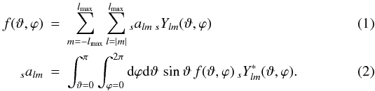 Equations (1) and (2) are known as backward (or synthesis) and
forward (or analysis) transforms, respectively. For a
discretised spherical map consisting of a vector p of
Npix pixels at locations
(ϑ,ϕ) and
with (potentially weighted) solid angles w, they change to:
Equations (1) and (2) are known as backward (or synthesis) and
forward (or analysis) transforms, respectively. For a
discretised spherical map consisting of a vector p of
Npix pixels at locations
(ϑ,ϕ) and
with (potentially weighted) solid angles w, they change to:
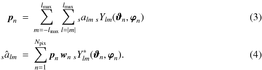 Depending
on the choice of lmax, w, and
the grid geometry, the
Depending
on the choice of lmax, w, and
the grid geometry, the  transform may only be
approximate, which is indicated by choosing the identifier â instead of
a.
transform may only be
approximate, which is indicated by choosing the identifier â instead of
a.
The main purpose of the presented code is the efficient implementation (regarding CPU time as well as memory consumption) of Eqs. (3) and (4) for scalars as well as tensor quantities of spins ±1 and ±2.
2.2. Design considerations
At present, several SHT implementations are in use within the CMB community, like those distributed with the Fortran and C++ implementations of HEALPix1 (Górski et al. 2005), GLESP2 (Doroshkevich et al. 2005), s2hat3, spinsfast4 (Huffenberger & Wandelt 2010), ccSHT5, and IGLOO6 (Crittenden & Turok 1998); they offer varying degrees of performance, flexibility and feature completeness. The main design goal for libpsht was to provide a code which performs better than the SHTs in these packages and is versatile enough to serve as a drop-in replacement for them.
This immediately leads to several technical and pragmatic requirements which the code must fulfill:
-
Efficiency:
the transforms provided by the library must perform atleast as well (in terms of CPU time and memory) as those in theavailable packages, on the same hardware. If possible, allavailable hardware features (like multiple CPU cores, vectorarithmetic instructions) should be used.
-
Flexibility:
the library needs to support all of the above discretisations of the sphere; in addition, it should allow transforms of partial maps.
-
Portability:
it must run on all platforms supported by the software packages above.
-
Universality:
it must provide a clear interface that can be conveniently called from all the programming languages used for the packages above.
-
Completeness:
if feasible, it should not depend on external libraries, because these complicate installation and handling by users.
-
Compactness:
in order to simplify code development, maintenance and deployment, the library source code should be kept as small as possible without sacrificing readability.
It should be noted that the code was developed as a library for use within other scientific applications, not as a scientific application by itself. As such it strives to provide a comprehensive interface for programmers, rather than ready-made facilities for users.
2.3. Supported discretisations
For completely general discretisations of the sphere, the operation count for SHTs is
 in both directions,
which is not really affordable for today’s resolution requirements. Fortunately,
approaches of lower complexity exist for grids with the following geometrical
constraints:
in both directions,
which is not really affordable for today’s resolution requirements. Fortunately,
approaches of lower complexity exist for grids with the following geometrical
constraints:
-
the map pixels are arranged on
 iso-latitude rings, where the colatitude of each ring is denoted as
ϑy;
iso-latitude rings, where the colatitude of each ring is denoted as
ϑy; -
within one ring, pixels are equidistant in ϕ and have identical weight wy; the number of pixels in each ring can vary and is denoted as Nϕ,y, and the azimuth of the first pixel in the ring is ϕ0,y.
Under these assumptions, Eqs. (3)
and (4) can be written as 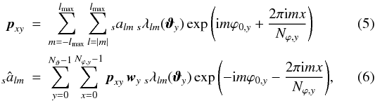 where
where
 . By subdividing both transforms
into two stages
. By subdividing both transforms
into two stages 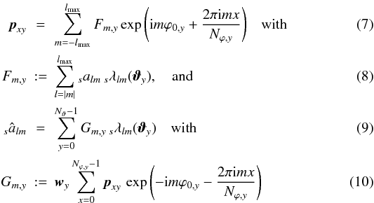 it
becomes obvious that the steps
it
becomes obvious that the steps  and
and
 require
 operations,
while a set of fast Fourier transforms – with the subdominant complexity of
operations,
while a set of fast Fourier transforms – with the subdominant complexity of
 –
can be used for the steps
Fm,y → pxy
and
pxy → Gm,y,
respectively. For any “useful” arrangement of the rings on the sphere,
Nϑ will be roughly proportional to
lmax, resulting in
–
can be used for the steps
Fm,y → pxy
and
pxy → Gm,y,
respectively. For any “useful” arrangement of the rings on the sphere,
Nϑ will be roughly proportional to
lmax, resulting in  operations per SHT.
Practically all spherical grids which are currently used in the CMB field (HEALPix, ECP, GLESP, IGLOO) fall into this category, so libpsht can take advantage of this simplification. A notable exception is the “quadrilateral spherical cube” grid used by the COBE mission, but this is not really an issue, since COBE’s resolution is so low that nowadays even brute-force SHTs produce results in acceptable time.
For the special case of the ECP grid, which is equidistant in both ϑ and
ϕ, algorithms of the even lower complexity
 have been
presented (see, e.g., Driscoll & Healy 1994;
Wiaux et al. 2007). These were not considered for
libpsht, because this would conflict with the flexibility goal. In addition, it has been
observed that the constant prefactor for these methods is fairly high, so that they do not
offer any performance advantage for small and intermediate
lmax; for transforms with high
lmax, on the other hand, their memory consumption is
prohibitively high.
have been
presented (see, e.g., Driscoll & Healy 1994;
Wiaux et al. 2007). These were not considered for
libpsht, because this would conflict with the flexibility goal. In addition, it has been
observed that the constant prefactor for these methods is fairly high, so that they do not
offer any performance advantage for small and intermediate
lmax; for transforms with high
lmax, on the other hand, their memory consumption is
prohibitively high.
2.4. Transformable quantities
Without limiting the general applicability of the provided SHTs, libpsht imposes a few constraints on the format of the data it processes. For scalar transforms, it will only work with real-valued maps (the ubiquitous scenario in CMB physics); this is not really a limitation, since transforming a complex-valued map can be achieved by simply transforming its real and imaginary parts independently and computing a linear combination of the results.
For SHTs with s ≠ 0, libpsht works on the so-called gradient
(E) and curl (B) components of the tensor field
 where
where
 ,
,
 and
(− 1)H is a sign convention (Lewis 2005). The default setting for H in libpsht is
1, following the HEALPix convention, but this can be changed easily if necessary. On the
real-space side, the tensor field is represented as two separate maps, containing the real
and imaginary part, respectively.
and
(− 1)H is a sign convention (Lewis 2005). The default setting for H in libpsht is
1, following the HEALPix convention, but this can be changed easily if necessary. On the
real-space side, the tensor field is represented as two separate maps, containing the real
and imaginary part, respectively.
In the following discussion, no fundamental distinction exists between
 and
and
 , so for the sake of
brevity both will be identified as
, so for the sake of
brevity both will be identified as  .
.
This choice of representation was made because it is compatible with the data formats
used by most existing packages, which simplifies interfacing and data exchange. It also
has the important advantage that any set of spherical harmonic coefficients is completely
specified by its elements with m >= 0, since
and
 are
coupled by symmetry relations.
are
coupled by symmetry relations.
3. Algorithm description
3.1. Calculation of the spherical harmonic coefficients
The central building block for every SHT implementation is the quick and accurate
computation of spherical harmonics  ; for libpsht, these need
only be evaluated at ϕ = 0 and will be abbreviated as
; for libpsht, these need
only be evaluated at ϕ = 0 and will be abbreviated as
 .
.
3.1.1. Scalar case
For s = 0, a proven method of determining the coefficients is using
the recursion relation  (13)with
 (14)in
the direction of increasing l; the starting values
λmm can be obtained from
λ00 = (4π)−1/2
and the additional recursion relation
(14)in
the direction of increasing l; the starting values
λmm can be obtained from
λ00 = (4π)−1/2
and the additional recursion relation
 (15)(Varshalovich et al. 1988). Since two values are
required to start the recursion in l, one also uses
(15)(Varshalovich et al. 1988). Since two values are
required to start the recursion in l, one also uses
 .
.
Both recursions are numerically stable; nevertheless, their evaluation is not trivial, since the starting values λmm can become extremely small for increasing m and decreasing sinϑ, such that they can no longer be represented by the IEEE754 number format used by virtually all of today’s computers. This problem was addressed using the approach described by Prézeau & Reinecke (2010), i.e. by augmenting the IEEE representation with an additional integer scale factor, which serves as an “enhanced exponent” and dramatically increases the dynamic range of representable numbers.
As is to be expected, this extended range comes at a somewhat higher computational cost; therefore the algorithm switches to standard IEEE numbers as soon as the λlm have reached a region which can be safely represented without a scale factor. From that point on, the recursion in l only requires three multiplications and one subtraction per λ value, which are very cheap instructions on current microprocessors.
From the above it follows that, depending on the exact parameters of the SHT, a
non-negligible fraction of the is extremely small, and
that all terms in Eqs. (8) and (9) containing such values as a factor do not
contribute in a measurable way to the SHT’s result, due to the limited dynamic range of
the floating-point format in which the result is produced. For that reason, libpsht
records the index lth, at which the
 first
exceed a threshold εth (which is set to the conservative
value of 10-30) during every l recursion. The remaining
operations will then be carried out for
l ≥ lth only.
first
exceed a threshold εth (which is set to the conservative
value of 10-30) during every l recursion. The remaining
operations will then be carried out for
l ≥ lth only.
Another acceleration is achieved by skipping the l-recursion for an (m,ϑ)-tuple entirely, if another recursion was performed before with mc ≤ m and |cosϑc| ≤ |cosϑ| < 1 that never crossed εth.
In the case that a ring at colatitude ϑ has a counterpart at
π − ϑ (which is almost always the case for the
popular grids), the recursion need only be
performed for one of those; the values for the other ring are quickly obtained by the
symmetry relation  (16)Libpsht will
identify such ring pairs automatically and treat them in an optimised fashion.
(16)Libpsht will
identify such ring pairs automatically and treat them in an optimised fashion.
3.1.2. Tensor case
Following Lewis (2005), libpsht does not
literally compute the tensor harmonics  , but rather their
linear combinations
, but rather their
linear combinations  (17)These are not
directly obtained using a recursion, but rather by first computing the spin-0
λlm and subsequently applying spin
raising and lowering operators; see Appendix A of Lewis
(2005) for the relevant formulae. Whenever scalar and tensor SHTs are performed
simultaneously, this has the advantage that the scalar
λlm can be re-used for both; in CMB
science this scenario is very common, since any transform involving a polarised sky map
requires SHTs for both s = 0 and s = ±2.
(17)These are not
directly obtained using a recursion, but rather by first computing the spin-0
λlm and subsequently applying spin
raising and lowering operators; see Appendix A of Lewis
(2005) for the relevant formulae. Whenever scalar and tensor SHTs are performed
simultaneously, this has the advantage that the scalar
λlm can be re-used for both; in CMB
science this scenario is very common, since any transform involving a polarised sky map
requires SHTs for both s = 0 and s = ±2.
The approach can be extended to higher spins in principle, but for
|s| > 2 the expressions become quite
involved and are also slow to compute. For this reason, libpsht’s transforms are
currently limited to s = 0, ±1, ±2.
Should a need for SHTs at higher s become evident, a method making use
of the relationships between  and the Wigner
 matrix elements
seems most promising, since they obey very similar recursion relations (see, e.g., Kostelec & Rockmore 2008), for which a recent
implementation is available (Prézeau & Reinecke
2010).
matrix elements
seems most promising, since they obey very similar recursion relations (see, e.g., Kostelec & Rockmore 2008), for which a recent
implementation is available (Prézeau & Reinecke
2010).
3.1.3. Re-using the computed
Many packages allow the user to supply an array containing precomputed
coefficients to the SHT
routines, which can speed up the computation by a factor of up to ≈2. Libpsht does not
provide such an option; this may seem surprising at first, but it was left out
deliberately for the following reasons:
-
Even if supplied externally, the coefficients have to be obtained bysome method. Reading them from mass storage is definitely not agood choice, since they can be computed on-the-fly much morequickly on current hardware. Externally provided values cantherefore only provide a benefit if they are used in at least twoconsecutive SHTs.
-
When using multiple threads in combination with precomputed
, computation time
soon becomes dominated by memory access operations to the table of coefficients,
because the memory bandwidth of a computer does not scale with the number of
processor cores. This will severely limit the scalability of the code. It is safe
to assume that this problem will become even more pronounced in the future, since
CPU power tends to grow more rapidly than memory bandwidth (Drepper 2007). -
For problem sizes with
 ,
when additional performance would be most desirable, the precomputed tables (whose
size is proportional to
,
when additional performance would be most desirable, the precomputed tables (whose
size is proportional to  ) become
so large that they no longer fit into main memory. A conservative estimate for the
size of the array at
lmax = 2000 and s = 0 is
about 8 GB; the Fortran HEALPix library currently requires 32GB in this situation.
) become
so large that they no longer fit into main memory. A conservative estimate for the
size of the array at
lmax = 2000 and s = 0 is
about 8 GB; the Fortran HEALPix library currently requires 32GB in this situation.
-
Libpsht supports multiple simultaneous SHTs, and will compute the
only once during such
an operation, re-using them for all individual transforms. Since this is done in a
piece-by-piece fashion (see Sect. 3.3), only
small subsets of size  need to be stored, which is more or less negligible; this approach also implies
that the internally precomputed subsets will most
likely remain in the CPU cache and therefore not be subject to the memory
bandwidth limit.
need to be stored, which is more or less negligible; this approach also implies
that the internally precomputed subsets will most
likely remain in the CPU cache and therefore not be subject to the memory
bandwidth limit.
3.2. Fast Fourier transform
Libpsht uses an adapted version of the well-known fftpack library (Swarztrauber 1982), ported to the C language (with a few minor
adjustments) by the author. This package performs well for FFTs of lengths
N whose prime decomposition only contains the factors 2, 3, and 5. For
prime N, its complexity degrades to
 ,
which should be avoided, so for N containing large prime factors,
Bluestein’s algorithm (Bluestein 1968) is employed,
which allows replacing an FFT of length N by a convolution (conveniently
implemented as a multiplication in Fourier space) of any length
≥2N − 1. By appropriate choice of the new length, the desired
,
which should be avoided, so for N containing large prime factors,
Bluestein’s algorithm (Bluestein 1968) is employed,
which allows replacing an FFT of length N by a convolution (conveniently
implemented as a multiplication in Fourier space) of any length
≥2N − 1. By appropriate choice of the new length, the desired
 complexity can be reestablished, at the cost of a higher prefactor.
Obviously it would have been possible to use the very popular and efficient FFTW7 library (Frigo &
Johnson 2005) for the Fourier transforms, but since this package is fairly
heavyweight, this would conflict with libpsht’s completeness or compactness goals. Even
though libfftpack with the Bluestein modification will be somewhat slower than FFTW, the
efficiency goal is not really compromised: libpsht’s algorithms have an overall complexity
of , so that the
FFT part with its total complexity of
will (for nontrivial problem sizes) never dominate the total CPU time.
3.3. Loop structure of the SHT
As Eqs. (5) and (6) and the complexity of
 already
suggest, a code implementing SHTs on an iso-latitude grid will contain at least three
nested loops which iterate on y, m, and
l, respectively. The overall speed and/or memory consumption of the
final implementation depend sensitively on the order in which these loops are nested,
since different hierarchies are not equally well suited for precomputation of common
quantities used in the innermost loop.
already
suggest, a code implementing SHTs on an iso-latitude grid will contain at least three
nested loops which iterate on y, m, and
l, respectively. The overall speed and/or memory consumption of the
final implementation depend sensitively on the order in which these loops are nested,
since different hierarchies are not equally well suited for precomputation of common
quantities used in the innermost loop.
The choice made for the computation of the , i.e. to obtain them by
l-recursion (see Sect. 3.1)
strongly favors placing the loop over l innermost; so only the order of
the y and m loops remains to be determined.
From the point of view of speed optimisation, arguably the best approach would be to
iterate over m in the outermost loop, then over the ring number
y, and finally over l. This allows precomputing the
Alm and
Blm quantities (see Sect. 3.1) exactly once and in small chunks, for an additional
memory cost of only .
However, this method requires additional  storage for the intermediate products Fm,y or
Gm,y, which is comparable to the size of
the input and output data. This was considered too wasteful, since it prohibits performing
SHTs whose input and output data already occupy most of the available computer memory.
storage for the intermediate products Fm,y or
Gm,y, which is comparable to the size of
the input and output data. This was considered too wasteful, since it prohibits performing
SHTs whose input and output data already occupy most of the available computer memory.
Unfortunately, switching the order of the two outermost loops does not improve the situation: now, one is presented with the choice of either precomputing the full two-dimensional Alm and Blm arrays, which is not acceptable for the same reason that prohibits storing the entire Fm,y and Gm,y arrays, or recomputing their values over and over, which consumes too much CPU time.
To solve this dilemma, it was decided not to perform the SHTs for a whole map in one go,
but rather to subdivide them into a number of partial transforms, each of which only deals
with a subset of rings (or ring pairs). An appropriate choice for the number of parts will
result in near-optimal performance combined with only small memory overhead; the most
symmetrical choice of  leads to a time overhead of
  and additional
memory consumption of
and additional
memory consumption of  , both of which are
small compared to the total CPU and storage requirements. Libpsht uses sub-maps of roughly
100 or Nϑ/10 rings (or
ring pairs), whichever is larger.
, both of which are
small compared to the total CPU and storage requirements. Libpsht uses sub-maps of roughly
100 or Nϑ/10 rings (or
ring pairs), whichever is larger.
The arrangement described above is sufficient for a single SHT. Since libpsht supports multiple simultaneous SHTs, another loop hierarchy had to be introduced. A pseudo-code listing illustrating the complete design of the SHT algorithm (including the subdominant parts performing the FFTs) is presented in Fig. 1.
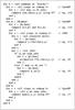 |
Fig. 1 Schematic loop structure of libpsht’s transform algorithm. |
3.4. Further acceleration techniques
To make use of multiple CPU cores, if available, the algorithm’s loop over m, as well as the code blocks performing the FFTs, have been parallelised using OpenMP8 directives, requesting dynamic scheduling for every iteration; this is indicated by the “OpenMP” tag in Fig. 1. As long as the SHTs are large enough, this results in very good scaling with the number of cores available (see also Sect. 5.2.4).
If the target machine supports the SSE2 instruction set9 (which is the case for all AMD/Intel CPUs introduced since around 2003), its
ability to perform two arithmetic operations of the same kind with a single machine
instruction is used to process two ring (pairs) simultaneously, greatly improving the
overall execution speed. The relevant loop is marked with “SSE2” in Fig. 1. The necessary changes are straightforward for the most
part; however, special attention must be paid to the l recursion, because
the two sequences of will cross the threshold to
IEEE-representable numbers at different lth. Fortunately this
complication can be addressed without a significant slowdown of the algorithm.
The data types used and the functions called in order to use the SSE2 instruction set are not part of the C90 language standard, and will therefore not be known to all compilers and on all hardware platforms. However there is a portable way to detect compiler and hardware support for SSE2; if the result of this check is negative, only the standard-compliant floating-point implementation of libpsht will be compiled, without the necessity of user intervention.
Similarly, the OpenMP functionality is accessed using so-called #pragma compiler directives, which are simply ignored by compilers lacking the required capability, reducing the source code to a single-threaded version.
Both extensions are supported by the widely used gcc10 and Intel compilers.
4. Programming interface
Only a high-level overview of the provided functionality can be given here. For the level of detail necessary to actually interface with the library, the reader is referred to the technical documentation provided alongside the source code.
4.1. Description of input/output data
Due to libpsht’s universality goal, it must be able to accept input data and produce output data in a wide variety of storage schemes, and therefore only makes few assumptions about how maps and alm are arranged in memory.
A tesselation of the sphere and the relative location of its pixels in memory is described to libpsht by the following set of data:
-
the total number of rings in the map; and
-
for every ring
-
the number of pixels Nϕ,y;
-
the index of the first pixel of the ring in the map array;
-
the stride between indices of consecutive pixels in this ring;
-
the azimuth of the first pixel ϕ0,y;
-
the colatitude ϑy;
-
the weight factor wy. This is only used for forward SHTs and is typically the solid angle of a pixel in this ring.
-
-
the maximum l and m quantum numbers available in the set;
-
the index stride between alm and al + 1,m;
-
an integer array containing the (hypothetical) index of the element a0,m.
Due to the convention described in Sect. 2.4, only coefficients with m ≥ 0 will be accessed.
These two descriptions are flexible enough to describe all spherical grids of interest, as well as all data storage schemes that are in widespread use within the CMB community. In combination with a data pointer to the first element of a map or set of alm, they describe all characteristics of a set of input or output data that libpsht needs to be aware of.
It should be noted that the map description trivially supports transforms on grids that only cover parts of the ϑ range; rings that should not be included in map synthesis or analysis can simply be omitted in the arrays describing the grid geometry, speeding up the SHTs on this particular grid. More general masks, which affect parts of rings, have to be applied by explicitly setting the respective map pixels to zero before map analysis or after map synthesis.
Libpsht will only work on data that is already laid out in main memory according to the structures mentioned above. There is no functionality to access data on mass storage directly; this task must be undertaken by the programs calling libpsht functionality. Given the bewildering variety of formats which are used for storing spherical maps and alm on disk – and with the prospect of these formats changing more or less rapidly in the future – I/O was not considered a core functionality of the library.
4.2. Supported floating-point formats
In addition to the flexibility in memory ordering, libpsht can also work on data in single- or double-precision format, with the requirement that all inputs and outputs for any set of simultaneous transforms must be of the same type. Internally, however, all computations are performed using double-precision numbers, so that no performance gain can be achieved by using single-precision input and output data.
4.3. Multiple simultaneous SHTs
As already mentioned, it is possible to compute several SHTs at once, independent of direction and spin, as long as their map and alm storage schemes described above are identical. This is achieved by repeatedly adding SHT requests, complete with pointers to their input and output arrays, to a “job list”, and finally calling the main SHT function, providing the job list, map information and alm information as arguments.
4.4. Calling the library from other languages
Due to the choice of C as libpsht’s implementation language, the library can be interfaced without any complications from other codes written in C or C++. Using the library from languages like Python and Java should also be straightforward, but requires some glue code.
For Fortran the situation is unfortunately a bit more complicated, because a well-defined interface between Fortran and C has only been introduced with the Fortran2003 standard, which is not yet universally supported by compilers. Due to the philosophy of incrementally building a job list and finally executing it (see Sect. 4.3), simply wrapping the C functions using cfortran.h11 glue code does not work reliably, so that building a portable interface is a nontrivial task. Nevertheless, the Fortran90 code beam2alm of the Planck mission’s simulation package has been successfully interfaced with libpsht.
5. Benchmarks
In order to evaluate the reliability and efficiency of the library, a series of tests and comparisons with existing implementations were performed. All of these experiments were executed on a computer equipped with 64GB of main memory and Xeon E7450 processors (24 CPU cores overall) running at 2.4 GHz. gcc version 4.4.2 was used for compilation.
5.1. Correctness and accuracy
The validation of libpsht’s algorithms was performed in two stages: first, the result of a backward transform was compared to that produced with another SHT library using the same input, and afterwards it was verified that a pair of backward and forward SHTs reproduces the original alm with sufficient precision.
All calculations in this section start out with a set of
 that consists
entirely of uniformly distributed random numbers in the range (−1;1), except for the
imaginary parts of the
that consists
entirely of uniformly distributed random numbers in the range (−1;1), except for the
imaginary parts of the  , which
must be zero for symmetry reasons, and coefficients with
l < |s|, which have no
meaning in a spin-s transform and are set to zero as well.
, which
must be zero for symmetry reasons, and coefficients with
l < |s|, which have no
meaning in a spin-s transform and are set to zero as well.
5.1.1. Validation against other implementations
For this test, a set of alm with lmax = 2048 was generated using the above prescription and converted to a Nside = 1024 HEALPix map by both libpsht and the Fortran HEALPix facility synfast. This was done for spins 0 and 2, mimicking the synthesis of a polarised sky map. Comparison of the resulting maps showed a maximum discrepancy between individual pixels of 1.55 × 10⁻⁷, and the RMS error was 6.3 × 10⁻¹³, which indicates a very good agreement.
5.1.2. Accuracy of recovered âlm
An individual accuracy test consists of a map synthesis, followed by an analysis of the
obtained map, producing the result  .
.
Two quantities are used to assess the agreement between these two sets of spherical
harmonic coefficients; they are defined as 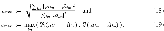 A
variety of such tests was performed for different grid geometries,
lmax, and spins; the results are shown in Figs. 2 and 3.
A
variety of such tests was performed for different grid geometries,
lmax, and spins; the results are shown in Figs. 2 and 3.
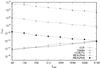 |
Fig. 2 εrms for libpsht transform pairs on ECP, Gaussian and HEALPix grids for various lmax. Every data point is the maximum error value encountered in transform pairs of all supported spins. “Healpix4” and “Healpix8” refer to iterative analyses with 4 and 8 steps, respectively. |
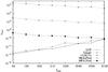 |
Fig. 3 εmax for libpsht transform pairs on ECP, Gaussian and HEALPix grids for various lmax. Every data point is the maximum error value encountered in transform pairs of all supported spins. “Healpix4” and “Healpix8” refer to iterative analyses with 4 and 8 steps, respectively. |
For ECP and “Gaussian” grids, each ring consisted of 2lmax + 1 pixels, and the grids contained 2lmax + 2 and lmax + 1 rings, respectively. The ϑy for the Gaussian grid were chosen to coincide with the roots of the Legendre polynomial Plmax + 1(ϑ). Under these conditions, and with appropriately chosen pixel weights (taken from Driscoll & Healy 1994; and Doroshkevich et al. 2005), the transform pair should reproduce the original alm exactly, were it not for the limited precision of floating-point arithmetics. In fact, the errors measured for SHTs on those two grids are extremely small and close to the theoretical limit.
For the transform pairs on HEALPix grids, a resolution parameter of
Nside = lmax/2
was chosen. Here, the recovered will only
be an approximation of the original ; if higher accuracy
is required, this approximation can be improved by Jacobi iteration, as described in the
HEALPix documentation. The figures show clearly that εrms is
around 10-3 for the simple transform pair and can be reduced dramatically by
iterated analysis.
5.2. Time consumption
5.2.1. Relative cost of SHTs
Single-core CPU time for various SHTs with lmax = 2048.
Table 1 shows the single-core CPU times for SHTs of different directions, spins and grids, but with identical band limit, in order to illustrate their relative cost. It is fairly evident that forward and backward SHTs with otherwise identical parameters require almost identical time, with the alm → map direction being slightly slower. Since this relation also holds for other band limits, only the timings for one direction will be shown in the following figures, in order to reduce clutter.
SHTs with |s| > 0 take roughly twice the
time of corresponding scalar ones; here the s = 2 case is slightly more
expensive than s = 1, because computing the
 from
λlm requires more operations than
computing the
from
λlm requires more operations than
computing the  .
.
The timings also indicate the scaling of the SHT cost with Nϑ, which is practically equal for HEALPix and ECP grids, but half as high for the Gaussian grid.
These timings, as well as all other timing results for libpsht in this paper, were obtained using SSE2-accelerated code. Switching off this feature will result in significantly longer execution times; on the benchmark computer the factor lies in the range of 1.6 to 1.8.
5.2.2. Scaling with lmax
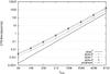 |
Fig. 4 Timings of single-core forward SHTs on a HEALPix grid with Nside = lmax/2. The annotation “polarised” refers to a combined SHT of spin 0 and 2 quantities, which is a very common case in CMB physics. |

SHTs of different spins and a wide range of band limits were performed on a single CPU
core, in order to assess the correlation between CPU time and
lmax; the results are shown in Fig. 4. As expected, the time consumption scales almost with
 ; deviations
from this behaviour only become apparent for lower band limits, where SHT components of
lower overall complexity (like the FFTs, computation of the
Alm and
Blm coefficients and initialisation of
data structures) are no longer negligible. Switching to a normalised representation of
the CPU time, as was done in Fig. 5, makes this
effect much more evident; even for transforms of very high band limit the curves are not
entirely horizontal, which would indicate a pure
; deviations
from this behaviour only become apparent for lower band limits, where SHT components of
lower overall complexity (like the FFTs, computation of the
Alm and
Blm coefficients and initialisation of
data structures) are no longer negligible. Switching to a normalised representation of
the CPU time, as was done in Fig. 5, makes this
effect much more evident; even for transforms of very high band limit the curves are not
entirely horizontal, which would indicate a pure  algorithm.
5.2.3. Performance comparison with Fortran HEALPix
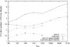 |
Fig. 6 CPU time ratios between the Fortran HEALPix synfast code and libpsht for various backward SHTs on a HEALPix grid with Nside = lmax/2. |
Figure 6 shows the ratio of CPU times for equivalent SHTs carried out using the synfast facility of Fortran HEALPix and libpsht, using identical hardware resources. It allows several deductions:
-
in all tested scenarios, libpsht’s implementation issignificantly faster, even when precomputed coefficients areused with synfast;
-
the performance gap is markedly wider for s = 0 transforms, which indicates that libpsht’s l-recursion is the part which has been accelerated by the largest factor in comparison to the Fortran HEALPix SHT library;
-
the polarised synfast SHTs only show a marginal speed improvement when using precomputed coefficients; for the scalar transforms, the difference is much more noticeable. Although this observation has no direct connection to libpsht, it is nevertheless of interest: most likely the missing acceleration is caused by saturation of the memory bandwidth, as discussed in Sect. 3.1.3, and confirms the decision not to introduce such a feature into libpsht.
5.2.4. Scaling with number of cores
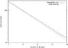 |
Fig. 7 Elapsed wall clock time for a backward SHT with s = 2, lmax = 4096, and Nside = 2048 on a HEALPix grid, run with a varying number of OpenMP threads. |
As illustrated in Fig. 1, all CPU-intensive parts of libpsht’s transform algorithm are instrumented for parallel execution on multicore computers using OpenMP directives. Figure 7 shows the wall clock times measured for a single SHT that was run using a varying number of OpenMP threads. The maximum number of threads was limited to 16 (in contrast to the maximum useful value of 24 on the benchmark computer), because the machine was not completely idle during the libpsht performance measurements, and the scaling behaviour at larger numbers of threads would have been influenced by other running tasks.
It is evident that the overhead due to workload distribution among several threads is quite small: for the 16-processor run, the accumulated wall clock time is only 18% higher than for the single-processor SHT. An analogous experiment was performed with the Fortran HEALPix code synfast; here the overhead for 16 threads was around 35%.
5.2.5. Comparison with theoretical CPU performance
For this experiment, the library’s code was enhanced to count the number of
floating-point operations that were carried out during the SHT. This instrumentation was
only done in the parts of the code with  complexity, i.e.
everything related to creation and usage of the . Operations that were
necessary only for the purpose of numerical stability (e.g. due to the range-extended
floating-point format) were not taken into account. Dividing the resulting number of
operations by the CPU time for a single-core uninstrumented run of the same SHT provides
a conservative estimate for the overall floating-point performance of the algorithm.
Measuring s = 0 and s = 2
alm → map SHTs on a HEALPix grid with
Nside = 1024 and lmax = 2048
resulted in 2.1GFlops/s and 4.1GFlops/s, respectively. This corresponds to 0.88 and 1.71
floating-point operations per clock cycle, or 22% and 43% of the theoretical peak
performance. Both of these percentages are quite high for an implementation of a
nontrivial algorithm, which can be seen as a hint that there is not much more room for
further optimisation on this hardware architecture. In other words, further speedups can
only be achieved by a fundamental change in the underlying algorithm.
complexity, i.e.
everything related to creation and usage of the . Operations that were
necessary only for the purpose of numerical stability (e.g. due to the range-extended
floating-point format) were not taken into account. Dividing the resulting number of
operations by the CPU time for a single-core uninstrumented run of the same SHT provides
a conservative estimate for the overall floating-point performance of the algorithm.
Measuring s = 0 and s = 2
alm → map SHTs on a HEALPix grid with
Nside = 1024 and lmax = 2048
resulted in 2.1GFlops/s and 4.1GFlops/s, respectively. This corresponds to 0.88 and 1.71
floating-point operations per clock cycle, or 22% and 43% of the theoretical peak
performance. Both of these percentages are quite high for an implementation of a
nontrivial algorithm, which can be seen as a hint that there is not much more room for
further optimisation on this hardware architecture. In other words, further speedups can
only be achieved by a fundamental change in the underlying algorithm.
There are several reasons for the obvious performance discrepancy between scalar and s = 2 transforms. To a large part it is probably caused by the internal dependency chains of the λlm recursion: even though the CPU could in principle start new operations every clock cycle, it has to wait for some preceding operations to finish first (which takes several cycles), because their results are needed in the next steps. When computing a recurrence, the CPU is therefore spending a significant fraction of time in a waiting state (see, e.g., Fog 2010). For the s = 2 transform this is much less of an issue, since many more floating-point operations must be carried out, which are not interdependent, and the time spent on the l-recursion becomes subdominant.
Other reasons for the lower performance of the recursion are the necessity to deal with extended floating-point numbers and its rather high ratio of memory accesses compared to arithmetic operations.
5.2.6. Gains by using simultaneous transforms
The CPU time savings achievable by performing multiple SHTs together instead of one after another were measured on a HEALPix grid with Nside = 1024 and lmax = 2048. Table 2 summarises the measured CPU times for an unsystematic selection of simultaneous and successive transforms, as well as the speedup.
Speedup for simultaneous vs. consecutive SHTs on a HEALPix grid with Nside = 1024 and lmax = 2048.
The results show that for a large number of simultaneous SHTs the computation time can
be cut roughly in half; this is the same asymptotic limit that also holds for SHTs with
completely precomputed (see Sect. 3.1.3), but the presented approach has dramatically
lower memory needs and can therefore be used for higher-resolution transforms. It is
also evident that forward and backward transforms, as well as transforms of different
spins, can be freely mixed while still preserving the performance increase.
5.3. Memory consumption
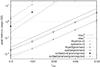 |
Fig. 8 Memory consumption of various SHTs performed with libpsht and synfast on a HEALPix grid with Nside = lmax/2. Input and output data are stored in single-precision format. |
Figure 8 shows the maximum amount of memory allocated during a variety of SHTs carried out using libpsht and the Fortran HEALPix synfast facility. Since the memory required for forward and backward transforms is essentially equal, only one direction has been plotted. The sizes of SHTs with lmax < 512 could not be measured reliably due to their short running time and are therefore not shown.
As can be seen, libpsht needs slightly less memory than synfast for equivalent
operations; overall, the scaling is very close to the expected
 if no
precomputed are used. For comparison
purposes, a few data points for synfast runs using precomputed scalar and tensor
were also plotted; they
clearly indicate the extremely high memory usage of these transforms, which scales with
.
if no
precomputed are used. For comparison
purposes, a few data points for synfast runs using precomputed scalar and tensor
were also plotted; they
clearly indicate the extremely high memory usage of these transforms, which scales with
.
During the tests with multiple simultaneous threads it was observed that increasing the number of cores does not have a significant influence on the total required memory; for the concrete test discussed in Sect. 5.2.4, memory usage for the run with 16 threads was only 2% larger than for the single-threaded run.
6. Conclusions
Looking back at the goals outlined in Sect. 2.2 and the results of the benchmark computations above, it can be concluded that the current version of the libpsht package meets almost all specified requirements. It implements SHTs that have the same or a higher degree of accuracy as the other available implementations, can work on all spherical grids relevant to CMB studies, and is written in standard C, which is very widely supported. The employed algorithms are significantly more efficient than those published and used in this field of research before; their memory usage is economic and allows transforms whose input and output data occupy almost all available space. When appropriate, vector capabilities of the CPUs, as well as shared memory parallelism are exploited, resulting in further performance gains.
Despite this range of capabilities, the package only consists of approximately 7000 lines of code, including the FFT implementation and in-line documentation for developers; except for a C compiler, it has no external dependencies.
Libpsht has been integrated into the simulation package of the Planck mission (Level-S, Reinecke et al. 2006), where it is interfaced with a development version of the C++ HEALPix package12 and a Fortran90 code performing SHTs on detector beam patterns; this demonstrates the feasibility of interfacing the library with C++ and Fortran code.
There are two areas in which libpsht’s functionality should probably be extended: it
currently does not provide transforms for spins larger than 2, and there is no active
support for distributing SHTs over several independent computing nodes. As was mentioned in
Sect. 3.1.2, addressing the first point is probably
not too difficult, and enhancing the library with  generators based on
Wigner d matrix elements is planned for one of the next releases. Regarding
the second point, a combination of libpsht’s central SHT functionality with the
parallelisation strategy implemented by Radek Stompor’s s2hat library appears very promising
and is currently being investigated.
generators based on
Wigner d matrix elements is planned for one of the next releases. Regarding
the second point, a combination of libpsht’s central SHT functionality with the
parallelisation strategy implemented by Radek Stompor’s s2hat library appears very promising
and is currently being investigated.
Libpsht is distributed under the terms of the GNU General Public License (GPL) version 2 (or later versions at the user’s choice); the most recent version, alongside online technical documentation can be obtained at the URL http://sourceforge.net/projects/libpsht/.
The next major release of HEALPix C++ will use libpsht.
Acknowledgments
Some of the results in this paper have been derived using the HEALPix (Górski et al. 2005) and GLESP (Doroshkevich et al. 2005) packages. M.R. is supported by the German Aeronautics Center and Space Agency (DLR), under program 50-OP-0901, funded by the Federal Ministry of Economics and Technology. I am grateful to Volker Springel, Torsten Ensslin, Jörg Rachen and Georg Robbers for fruitful discussions and valuable feedback on drafts of this paper.
References
- Bluestein, L. I. 1968, Northeast Electronics Research and Engineering Meeting Record, 10, 218 [Google Scholar]
- Crittenden, R. G., & Turok, N. G. 1998 [arXiv:astro-ph/9806374], unpublished [Google Scholar]
- Doroshkevich, A. G., Naselsky, P. D., Verkhodanov, O. V., et al. 2005, Int. J. Mod. Phys. D, 14, 275 [NASA ADS] [CrossRef] [Google Scholar]
- Drepper, U. 2007, What Every Programmer Should Know About Memory, http://www.akkadia.org/drepper/cpumemory.pdf [Google Scholar]
- Driscoll, J. R., & Healy, D. M. 1994, Adv. Appl. Math., 15, 202 [CrossRef] [Google Scholar]
- Fog, A. 2010, Optimizing software in C++, http://agner.org/optimize/optimizing_cpp.pdf [Google Scholar]
- Frigo, M., & Johnson, S. G. 2005, Proc. IEEE, 93, 216, http://fftw.org/fftw-paper-ieee.pdf [Google Scholar]
- Górski, K. M., Hivon, E., Banday, A. J., et al. 2005, ApJ, 622, 759 [NASA ADS] [CrossRef] [Google Scholar]
- Huffenberger, K. M., & Wandelt, B. D. 2010, ApJS, 189, 255 [NASA ADS] [CrossRef] [Google Scholar]
- Kostelec, P., & Rockmore, D. 2008, J. Fourier Analysis and Applications, 14, 145 [CrossRef] [Google Scholar]
- Lewis, A. 2005, Phys. Rev. D, 71, 083008 [NASA ADS] [CrossRef] [Google Scholar]
- Prézeau, G., & Reinecke, M. 2010, ApJS, 190, 267 [NASA ADS] [CrossRef] [Google Scholar]
- Reinecke, M., Dolag, K., Hell, R., Bartelmann, M., & Enßlin, T. A. 2006, A&A, 445, 373 [NASA ADS] [CrossRef] [EDP Sciences] [Google Scholar]
- Swarztrauber, P. 1982, Vectorizing the Fast Fourier Transforms (New York: Academic Press), 51 [Google Scholar]
- Varshalovich, D. A., Moskalev, A. N., & Khersonskii, V. K. 1988, Quantum Theory of Angular Momentum (World Scientific Publishers) [Google Scholar]
- Wiaux, Y., Jacques, L., & Vandergheynst, P. 2007, J. Comput. Phys., 226, 2359 [NASA ADS] [CrossRef] [Google Scholar]
All Tables
Speedup for simultaneous vs. consecutive SHTs on a HEALPix grid with Nside = 1024 and lmax = 2048.
All Figures
|
Fig. 1 Schematic loop structure of libpsht’s transform algorithm. |
| In the text | |
|
Fig. 2 εrms for libpsht transform pairs on ECP, Gaussian and HEALPix grids for various lmax. Every data point is the maximum error value encountered in transform pairs of all supported spins. “Healpix4” and “Healpix8” refer to iterative analyses with 4 and 8 steps, respectively. |
| In the text | |
|
Fig. 3 εmax for libpsht transform pairs on ECP, Gaussian and HEALPix grids for various lmax. Every data point is the maximum error value encountered in transform pairs of all supported spins. “Healpix4” and “Healpix8” refer to iterative analyses with 4 and 8 steps, respectively. |
| In the text | |
|
Fig. 4 Timings of single-core forward SHTs on a HEALPix grid with Nside = lmax/2. The annotation “polarised” refers to a combined SHT of spin 0 and 2 quantities, which is a very common case in CMB physics. |
| In the text | |
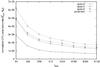 |
Fig. 5 Same as Fig. 4, but with CPU time divided by
|
| In the text | |
|
Fig. 6 CPU time ratios between the Fortran HEALPix synfast code and libpsht for various backward SHTs on a HEALPix grid with Nside = lmax/2. |
| In the text | |
|
Fig. 7 Elapsed wall clock time for a backward SHT with s = 2, lmax = 4096, and Nside = 2048 on a HEALPix grid, run with a varying number of OpenMP threads. |
| In the text | |
|
Fig. 8 Memory consumption of various SHTs performed with libpsht and synfast on a HEALPix grid with Nside = lmax/2. Input and output data are stored in single-precision format. |
| In the text | |
Current usage metrics show cumulative count of Article Views (full-text article views including HTML views, PDF and ePub downloads, according to the available data) and Abstracts Views on Vision4Press platform.
Data correspond to usage on the plateform after 2015. The current usage metrics is available 48-96 hours after online publication and is updated daily on week days.
Initial download of the metrics may take a while.