| Issue |
A&A
Volume 526, February 2011
|
|
|---|---|---|
| Article Number | A124 | |
| Number of page(s) | 11 | |
| Section | Stellar atmospheres | |
| DOI | https://doi.org/10.1051/0004-6361/201015769 | |
| Published online | 10 January 2011 | |
Spectral analysis of Kepler SPB and β Cephei candidate stars⋆
1
Thüringer Landessternwarte Tautenburg,
07778
Tautenburg,
Germany
e-mail: lehm@tls-tautenburg.de; andrew@tls-tautenburg.de
2
GEPI, Observatoire de Paris, CNRS, Université Paris
Diderot, 5 place Jules
Janssen, 92190
Meudon,
France
e-mail: thierry.semaan@obspm.fr
3
Instituto de Astrofísica de Andalucía (CSIC),
Apartado 3004, 18080
Granada,
Spain
e-mail: jgs@iaa.es
4
Astrophysics Group, Keele University, Staffordshire
ST5 5BG,
UK
e-mail: bs@astro.keele.ac.uk
5 Instituut voor Sterrenkunde,
Katholieke Universiteit Leuven, Belgium
e-mail: maryline@ster.kuleuven.be
6
Georg-August-University, Göttingen, Germany
e-mail: denis.shulyak@gmail.com
7
Tavrian National University, Department of
Astronomy, Simferopol,
Ukraine
e-mail: vadim@starsp.org
8 Royal Observatory of
Belgium
e-mail: Peter.DeCat@oma.be
Received:
16
September
2010
Accepted:
11
November
2010
Context. For asteroseismic modelling, analysis of the high-accuracy light curves delivered by the Kepler satellite mission needs support by ground-based, multi-colour and spectroscopic observations.
Aims. We determine the fundamental parameters of SPB and β Cep candidate stars observed by the Kepler satellite mission and estimate the expected types of non-radial pulsators.
Methods. We compared newly obtained high-resolution spectra with synthetic spectra computed on a grid of stellar parameters assuming LTE, and checked for NLTE effects for the hottest stars. For comparison, we determined Teff independently from fitting the spectral energy distribution of the stars obtained from the available photometry.
Results. We determine Teff, log g, microturbulent velocity, vsini, metallicity, and elemental abundance for 14 of the 16 candidate stars. Two stars are spectroscopic binaries. No significant influence of NLTE effects on the results could be found. For hot stars, we find systematic deviations in the determined effective temperatures from those given in the Kepler Input Catalogue. The deviations are confirmed by the results obtained from ground-based photometry. Five stars show reduced metallicity, two stars are He-strong, one is He-weak, and one is Si-strong. Two of the stars could be β Cep/SPB hybrid pulsators, four SPB pulsators, and five more stars are located close to the borders of the SPB instability region.
Key words: asteroseismology / stars: early-type / stars: variables: general / stars: atmospheres / stars: abundances
© ESO, 2011
1. Introduction
List of observed stars.
The Kepler satellite delivers light curves of unique accuracy and time coverage, providing unprecedented data for the asteroseismic analysis. The identification of non-radial pulsation modes and the asteroseismic modelling, on the other hand, require a classification of the observed stars in terms of Teff, log g, vsini, and metallicity. These basic stellar parameters cannot be obtained using only Kepler’s single-bandpass photometry. But they can be deduced from multi-colour photometry and from spectroscopy and that is why ground-based observations of the Kepler target stars are urgently needed.
We describe a semi-automatic method of spectrum analysis based on the high-resolution spectra of 16 stars (Sect. 2), taken from a list of 34 brighter B-type stars in the Kepler satellite field of view that have been proposed by the Working Groups 3 and 6 of the Kepler Asteroseismic Science Consortium (KASC) to be candidates for SPB and β Cep pulsators. For the object selection, the Teff and log g values given in the Kepler Input Catalogue1 (KIC) were used in most cases (Balona et al. 2010). Our sample comprises the 16 brightest stars from the original selection, which meanwhile has been expanded to 49 candidate stars. The Teff and log g values listed in the KIC are based on Sloan Digital Sky Survey-like griz, D51 (510 nm) and 2MASS JHK photomety (Batalha et al. 2010). The noted passbands do not contain the Balmer-jump, which leads to inaccurate parameters for the hotter stars. There are therefore hints that the temperature values given in the KIC show larger deviations for stars hotter than about 7000 K (see Molenda-Żakowicz et al. 2010). Moreover, the surface gravity given in the KIC has an uncertainty of ±0.5 dex, which is much too high for an accurate classification of the stars in terms of non-radial pulsators. The spectral types given for most of the selected stars in the SIMBAD database, operated at the CDS, Strasbourg, are based on only a few, older measurements and in most cases no luminosity class can be found. For two stars we found no classification in the SIMBAD database and for two no classification in the KIC.
The aim of this work is to provide fundamental stellar parameters like effective temperature Teff, surface gravity log g, metallicity [M/H], and projected rotation velocity vsini for an asteroseismic modelling of the stars, to compare our results of spectral analysis with the KIC data and to estimate the expected type of variability of the different target stars. For the analysis, we used stellar atmosphere models and synthetic spectra computed under the assumption of local thermodynamic equilibrium (LTE, Sect. 3). However, since non-LTE (NLTE) effects may be important for the hotter B-type stars (see e.g. Auer & Mihalas 1973), we repeated the analysis for the three hottest stars in our sample using NLTE computations (Sect. 4). The comparison of results allowed us to evaluate the importance of NLTE effects and the reliability of our LTE analysis. An additional comparison was performed with those stellar temperatures obtained using the spectral energy distributions (SEDs) derived from multi-colour photometry of the stars (Sect. 5). Finally, we compared the derived stellar parameters with those expected for SPB and β Cep pulsators from theoretical computations (Sect. 6). The results are discussed in the corresponding sections and summarized in Sect. 7.
2. Observations
Spectra of 16 bright (V < 10.4) suspected SPB and β Cep stars selected from the KIC have been taken with the Coude-Echelle spectrograph attached to the 2-m telescope at the Thüringer Landessternwarte (TLS) Tautenburg. The spectra have a resolving power of 32 000 and cover the wavelength range from 470 to 740 nm. Table 1 gives KIC number, common designation, suspected type of variability, V-magnitude, number of observed spectra, and the signal-to-noise of the averaged spectra for all observed stars. The last three columns list the spectral types given in the SIMBAD database, the inferred spectral types derived from the Teff and log g given in the KIC, and derived from the results of our analysis (Sect. 3.3). For the derivation we used the tables by Schmidt-Kaler (1982) and by de Jager & Nieuwenhuijzen (1987).
Spectra have been reduced using standard ESO-MIDAS packages. In addition, we accounted for small shifts of the instrumental radial velocity (RV) zero point by comparing the positions of a large number of telluric O2-lines with their known wavelengths and corrected the spectra for the observed deviations. Finally, the RV differences between all the spectra of the same star have been determined from cross-correlation, and the spectra rebinned according to theses differences and added to build the mean, averaged spectrum.
Number of stronger lines in ionization stages I to III in the considered spectral region for stars of 10 000 K and 20 000 K.
 |
Fig. 1 Observed (black) and synthetic (red) spectra (normalized intensity versus wavelength in Å) of KIC 8 451 410. |
3. LTE based analysis
3.1. The method
The large vsini of many of the observed stars makes it impossible to find enough unblended spectral lines for a spectral analysis based on the comparison of the equivalent widths of the lines of single elements. Thus we decided to analyse the spectra by computing synthetic spectra for a wider spectral region, including Hβ and more of metal lines.
A necessary precondition for using the spectrum synthesis method to derive unique values of Teff and log g independently of the elemental abundances is to have a sufficient number of lines of elements in different ionization stages. We used the spectral range from 472 to 588 nm (lower end of the covered wavelength range up to the wavelength where stronger telluric lines occur). Table 2 lists the number of lines present in the considered spectral region, and they show line depths of the intrinsic, rotationally unbroadened lines of more than 5%, calculated with the SynthV program (see below) for stars of 10 000 and 20 000 K. Numbers given in bold face indicate that there are lines of the corresponding element in different ionization stages. It can be seen that the temperature of the cooler stars can be determined from the ionization balance between Fe i and Fe ii and minor contributions from the Ca, Cr, Mg, and Ni lines, and from the Fe ii/Fe iii and Si ii/Si iii stages for the hotter stars. Figure 1 shows a cut-off from the observed and calculated spectra of KIC 8 451 410, one of the cooler target stars showing sharp lines. The ions of the stronger lines are indicated, among them the main diagnostic lines of Fe i and Fe ii.
 |
Fig. 2 χ2 obtained from the grid search in five parameters versus three of the parameters. |
We used the LLmodels program (Shulyak et al. 2004) in its most recent parallel version to compute the atmosphere models and the SynthV program (Tsymbal 1996) in a parallelized version written by A.T. to compute the synthetic spectra. The LLmodels code is a 1-D stellar model atmosphere code for early and intermediate type stars assuming LTE that is intended for as accurate a treatment as possible of the line opacity using a direct method for the line-blanketing calculation. This line-by-line method is free of any approximations so that it fully describes the dependence of the line absorption coefficient on frequencies and depths in a model atmosphere, it does not require precalculated opacity tables. The code is based on modified ATLAS9 subroutines (Kurucz 1993a) and the continuum opacity sources and partition functions of iron-peak elements from ATLAS12 (Kurucz 1993b) are used. The advantage of the programs in our application is that they allow us to use different metallicity and individual abundances of He and metals and that they run fast in parallel mode on a cluster PC installed at TLS. The main limitation with respect to hot stars is that both programs assume LTE. The line tables have been taken from the VALD data base (Kupka et al. 2000). They were adjusted by the mentioned programs according to the different spectral types.
We computed the synthetic spectra on a grid in Teff, log g, vsini, and metallicity, based on a pre-calculated library of atmosphere models. The models were computed by scaling the solar abundance taken from Grevesse et al. (2007) of each metal by −0.8 to +0.8 dex, assuming constant, solar He abundance and a microturbulent velocity of 2 km s-1. In the following, metallicity [M/H] means this abundance difference in dex compared to the solar value, valid for all metals. The value of [M/H] was derived in this step and will be given later in Table 5 together with the other parameters.
In a second step, we fixed the previously derived parameters to its optimum values and took the abundance table corresponding to the determined metallicity as the starting point for readjusting the individual abundances of He and selected metals. All the abundances of these single elements have been derived from the spectrum synthesis method. First, we checked for the presence of lines of the corresponding element in the spectrum of the star by computing a synthetic spectrum that only includes the lines of H, He, and the single element and compared it with the observed one. Then, if lines of this element could be detected, we iterated its abundance together with vsini until we reached a new minimum in the χ2 calculated from the comparison with the observed spectrum.
In the final step, we readjusted the values of Teff, log g, and vsini based on the abundances determined in step two and added the microturbulent velocity ξt as a free parameter. We were not able to compute all the atmosphere models for the full parameter space including the individual abundances of He and metal lines and different ξt, however. We used the atmosphere models computed for the fixed, optimum metallicity determined in step 1 but computed the synthetic spectra with the SynthV program based on the individual abundances determined in step 2. A comparison of the derived metallicities and metal abundances showed that the derived values are compatible in most cases. Only for the three stars where we found larger deviations of the He abundance (the He weak star KIC 5 479 821 and the He strong stars KIC 8 177 087 and KIC 12 258 330) did we have to calculate and use atmosphere models based on exactly the determined He abundances. The final values of the parameters and its errors have been taken from step 1 for the metallicity, from step 2 for the individual abundances (here, we did no error calculation but assumed the error derived for the metallicity to be the typical error), and from the last step for all the other parameters.
The applied method of grid search allows finding the global minimum of χ2 and for a realistic estimation of the errors of the parameters as we show in the next section.
3.2. Testing the method
The method was tested on a spectrum of Vega (spectral type A0 V, Morgan & Keenan 1973) taken with the same instrument and spectral resolution, with the aim of checking for the reliability of the obtained values and for the influence of the different parameters on the accuracy of the results. Figure 2 shows the χ2-distributions obtained from the grid search. Each panel contains all χ2 values up to a certain value obtained from all combinations of the different parameters versus one of the parameters. The dashed lines indicate the 1σ confidence level obtained from the χ2-statistics assuming that the χ2-distribution approaches a Gaussian one when the number of degrees of freedom is high. The continuous curves show the polynomial fit to the lowest χ2-values. The three crosses in each panel show the optimum value and the ±1σ error limits of the corresponding parameter.
Vega: comparison of the results. Errors of our determination are given in the last row.
Table 3 lists the resulting values and compares them with results from the literature. Our values of Teff and log g agree well with those from previous investigations. The metallicity and microturbulent velocity have been used by us as free parameters as well. The obtained values confirm those assumed by the other authors and the obtained value of vsini is identical with that measured by Hill et al. (2004).
We also used this test to check for the influence of a given parameter on the determination of the other ones. A simple way to look for such correlations is to compute the optimum values of all N parameters and their errors first by doing a search on the full grid of parameters. Then one of the parameters is fixed to its derived optimum value and the optimization of the other parameters is repeated on an N-1 grid. The obtained values will be the same but the derived error will be smaller the more the corresponding parameter is correlated with the parameter that was fixed. Table 4 gives in each row the fraction of the computed error of the parameters in the case where one of them is fixed to the error that is obtained when all parameters are considered to be free. The values indicating the strongest effects are set in bold face. It shows that there is a strong correlation between Teff, log g, and metallicity (cases 1, 3, and 4). This can be easily understood because the line strengths are determined by Teff and [M/H] and the shape of the Balmer line is strongly influenced by log g and [M/H]. Both vsini and ξt, on the other hand, are much less influenced by the other parameters and fixing them to their optimum values in the error calculation has no effect on the derived errors of the other parameters (cases 2 and 5). The result shows that we have to vary at least Teff, log g, and metallicity together to get reliable results and error estimations.
 |
Fig. 3 Error in ξt versus measured Teff. |
Reduction in the errors of the parameters in % by fixing one of them (see text).
Fundamental parameters.  and
log gK are taken from the KIC and given for
comparison.
and
log gK are taken from the KIC and given for
comparison.
Metallicity and elemental abundances relative to solar ones in dex and He abundance in fractions of the solar one. Stars are sorted by Teff.
3.3. Results
Table 5 lists the fundamental parameters obtained for the 16 target stars. For comparison Teff and log g taken from the KIC are given. The accuracy in Teff is about 2% (mean value of 1.8%) for most of the stars, but only for the two hottest stars do we obtain twice this value. Looking for any correlations between the errors of measurement and the absolute values of determined parameters, we found only one, namely for the microturbulent velocity in dependence on Teff (Fig. 3). It seems that our method can determine ξt with an accuracy of about 0.6 km s-1 for the cooler stars, but that the error rises to almost 4 km s-1 for the hottest stars. It means that, for stars hotter than about 15 000 K, it is not possible to determine their microturbulent velocity and that for those stars the determination of the other parameters is practically independent of the value of ξt. There is also a slight correlation between the relative error of vsini and log g that we attribute to the fact that the accuracy of vsini is lowered by including Hβ in the measurement and that for lower log g the Balmer lines show narrower profiles. A test of two of the stars of different temperatures shows that the determination of vsini by excluding Hβ gives the same values but with smaller errors. Thus, the vsini measurement can be done independently of the log g determination for which one includes the Balmer lines, and our given errors (mean accuracy of 8%) are overestimated. The mean error in log g is of 0.07. We refer to the previous section where it was shown that all the errors get larger (and more reliable) by determining them from the complete grid in all parameters as we did here.
Table 6 lists the resulting metallicities and individual abundances. The upper part gives the abundances of elements that were found in the spectra of most of the stars, the lower part those that have also been found for the cooler stars. Larger deviations from the solar values are highlighted in bold face. The solar values refer to the solar chemical composition given by Grevesse et al. (2007). In the following, we remark on peculiarities found in some of the stars. A general comparison of our results with the KIC data will be given in the next section.
KIC 3 240 411 and 10 960 750: not any data about these two stars from previous investigations could be found. According to our measurement, they are the hottest stars of our sample. KIC 3 240 411 has low metallicity, in agreement with a distinct depletion in Fe, whereas KIC 10 960 750 has solar abundance.
KIC 3 756 031: this star shows the lowest metallicity of our sample. All metals where we found contributions in its spectrum are depleted, whereas He is enhanced. The profiles of some of the metal lines are strongly asymmetric. This may indicate pulsation (we will show that the star falls into the SPB instability region) or, because of the chemical peculiarity of the star, rotational modulation due to spots (as found, e.g., by Briquet et al. (2004) for four B-type stars showing inhomogeneous surface abundance distributions).
KIC 5 217 845: the star has been identified from the Kepler satellite light curve as eclipsing binary of uncertain type with a period of 1.67838 days (Prsa et al. 2010). No RV or line profile variations could be detected from our two spectra, however.
KIC 5 479 821: the star is He-weak by a factor of 0.46 compared to the solar value. It shows a strong enhancement of C and N and a depletion of Mg and S. All final parameter values have been calculated from atmosphere models based on the derived individual abundances. The given metallicity, derived from a previous step, has no physical meaning.
KIC 8 177 087: this is the sharpest-lined star of our sample with vsini = 22 km s-1. Whereas He is strongly enhanced, all metal abundances are close to the solar values.
KIC 8 451 410: this is a suspected SB2 star. We observe an RV shift between our two spectra and cannot fit the shifted and co-added spectrum as perfectly as in the other cases. The observed strong Ba and Y overabundance and the strong depletion in Sc may be related to the presence of a second component in the observed spectrum. The determined low temperature of about 8 500 K agrees within the errors of measurement with that given in the KIC.
KIC 8 459 899: from the slightly larger O-C residuals of the spectrum fit, we suspect that this star may be an SB2 star as well but that the obtained parameters are still reliable. It has low metallicity, and the derived value agrees well with the depleted metal abundances, except for O, which is enhanced.
KIC 8 583 770: this is a double star (WDS 19570+4441) with a 3-magnitude fainter companion at a separation of 0.9″. According to our analysis, it is Si-strong, and Mg is enhanced.
KIC 8 766 405: the star has low metallicity, the derived value agrees well with the depleted metal abundances, except for N and O which are enhanced.
KIC 11 973 705: this is certainly an SB2 star, and the typical spectrum of a cooler star of 8000 to 9000 K can be seen in the O-C residuals. All values given here result from a formal solution for the hotter component that shows the stronger lines. Due to the unknown flux ratio between the two components, the derived values are not reliable, except for vsini.
KIC 12 207 099: for this sharp-lined star we have got no satisfactory solution. Maybe that it is a chromium star (we obtain a Cr abundance of 2.30 dex above the solar one) and vertical stratification of the elemental abundances has to be included in the calculations, or it is an SB2 star as well.
KIC 12 258 330: the star is He-strong, and it shows an enhancement in He abundance by a factor of more than two compared to the solar value. The metal abundances are close to the solar values, and the derived metallicity is too low (see the remark for KIC 5 479 821).
3.4. Comparison with the KIC data
Comparing our Teff and log g with the values given for 12 of the stars in the KIC (for two of the 16 stars of our sample there are no entries, and we excluded KIC 11 973 705 and 12 207 099), we see systematic differences. We obtain higher temperatures in general, and the difference increases with increasing temperature of the stars. Already Molenda-Żakowicz et al. (2010) have found that the Teff given in the KIC is too low for stars hotter than about 7000 K, by up to 4000 K for the hottest stars. The trend in the temperature difference derived from our values is shown in Fig. 4. The error in the difference also includes the 200 K error typical for the KIC data. We have drawn the curve of a second order polynomial resulting from a fit that observes the boundary condition that the difference should be zero for Teff = 7000 K. Our analysis seems to confirm the finding by Molenda-Żakowicz et al.
 |
Fig. 4 Difference in Teff between our values and those given in the KIC versus measured Teff. |
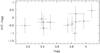 |
Fig. 5 Difference in log g between our values and those given in the KIC versus measured log g. |
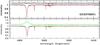 |
Fig. 6 Fit (red) of the spectrum of K03758031 (black), assuming Teff=16 000 K (top) and Teff=11 200 K (bottom). The O−C spectra are shifted by +1.1. |
Comparing our values derived for log g with those given in the KIC shows that they are systematically lower (Fig. 5). Due to the large errors that mainly result from the ± 0.5 dex error of the KIC data, we cannot say that this difference is significant, however. The same holds true for the Fe/H ratios given in the KIC, because the corresponding error of ± 0.5 dex prevents us from any comparison with our derived values.
There are two extreme cases: KIC 3 756 031, where our derived temperature is 16 000 K whereas the KIC gives about 11 200 K and KIC 12 258 330, where we obtain a log g of 3.85, which is lower by 1 dex than given in the KIC. A closer investigation shows, however, that the KIC values are very unlikely.
Figure 6 shows, in its upper panel, the fit of a part of the spectrum of KIC 3 756 031 assuming our value of Teff. The lower panel gives the same for Teff taken from the KIC. Neither Hβ nor the He lines are fitted well. The best fit of Hβ at this temperature is obtained assuming a log g below 3.0, but in this case the He lines can also not be reproduced. The use of LTE in our program cannot balance a temperature difference of 5000 K, and the 11200 K given in the KIC cannot be true for this star.
 |
Fig. 7 As in Fig. 6 but for KIC 12 258 330 and Teff = 14 750 K, log g = 3.85 (top) and Teff = 13 224 K, log g = 4.86 (bottom). |
Figure 7 shows, in its upper panel, the fit of a part of the spectrum of KIC 12 2583 330 assuming our values of Teff and log g. The lower panel gives the same for Teff and log g taken from the KIC. The resulting deviation in the shape of Hβ cannot be explained in terms of a wrong continuum normalization in the Hβ range. The log g given for this star in the KIC is by about 1 dex too large.
4. NLTE based analysis
4.1. The method
Our aim in this attempt was not to investigate the NLTE effects in detail but to check for the order of the deviations in the results of the LTE calculations that may arise from neglecting these effects. We used the GIRFIT program (Frémat et al. 2006) to determine the fundamental parameters Teff, log g, and vsini. This program adjusts synthetic spectra interpolated on a grid of stellar fluxes to the observed spectra using the least squares method. The temperature structure of the atmospheres was computed as in Castelli & Kurucz (2003) using the ATLAS9 computer code (Kurucz 1993a). Non-LTE level populations were then computed for each of the atoms listed in Table A.1 (only available in the electronic version) using the TLUSTY program (Hubeny & Lanz 1995) and keeping the temperature and the density distributions obtained with ATLAS9 fixed. For the spectral region considered, we used the specific intensity grids computed by Frémat (private communication) for Teff and log g ranging from 15 000 K to 27 000 K and from 3.0 to 4.5, respectively. For Teff < 15 000 K we used LTE calculation. We assumed solar metallicity and a micro-turbulence of 2 km s-1 for all the grids.
Our investigation of NLTE effects in the three hottest stars of our sample (not regarding the suspected SB2 candidates) is based on the 4720–5050 Å spectral region. For the two hotter stars, KIC 3 240 411 and KIC 10 960 750, we used the two helium lines at 4921 and 5016 Å that are present in this region to measure vsini. Then we determined the other parameters, Teff and log g, by fitting the spectrum in the whole domain between 4720 and 5050 Å. For the cooler star KIC 3 756 031, the determination of vsini is based on the metallic and the He I lines. The derived vsini values of these stars are consistent with those obtained for the Hβ lines. Additionally, we used the spectrum of KIC 12 258 330 for an analysis with the above-mentioned programs but in LTE to check for the influence of using different wavelength ranges and the differences in the applied programs. For this star, we derived Teff = 14 700 K (Sect. 3.3) and we do not expect NLTE effects at this temperature.
4.2. Results
Table 7 lists the results. The given errors were computed according to the error determination method introduced by Martayan et al. (2006), which is based on computing theoretical spectra where a Poisson-distributed noise has been added. For KIC 12 258 330, we did not find any satisfying solution that fits both the Balmer and the He lines, so we give two solutions here. For comparison, we also list the parameter values obtained in Sect. 3 and visualize the differences in the results in Fig. 8. The values of vsini derived from the two different methods agree within the errors of measurement for all of the stars.
 |
Fig. 8 Comparison of the parameter values derived from LTE (crosses) and from NLTE (circles) treatment. |
Fundamental parameters derived from the NLTE model (LTE for KIC 12 258 330).
For two of the stars, among them the hottest star KIC 3 240 411, the values of both Teff and log g agree within the errors of measurement. For the other two stars, surprisingly for KIC 12 258 330 where we assumed LTE, we observe large differences between the values obtained from the two approaches.
4.3. Discussion of the influence of NLTE effects
Four stars were analysed by two different methods using a) slightly different input physics; b) LTE or NLTE treatment for three of the stars; and c) different wavelength ranges, short in NLTE, and wider in LTE. For two of the stars, KIC 3 240 411 and KIC 3 766 081, the results agree well within the errors of measurement. For the other two stars, KIC 10 960 750 and KIC 12 258 330, we find significant deviations. That we find a good agreement for the hottest star and a distinct deviation for the coolest one that was analysed using LTE in both attempts is surprising and raises questions about the origin of the observed deviations, i.e. about the level of the influence of the differences in the two methods that we labelled a) to c) in before.
For KIC 12 258 330, we can clearly show that the difference in the results comes from its beeing a helium-strong star and that our second approach assumed solar metallicity and He abundance. A change in He abundance modifies the structure of the stellar atmosphere (temperature and density), so the derived Teff and log g will depend on the He abundance, apart from any NLTE effect. Figure 9 shows the quality of different fits, all calculated in LTE. Model 1 is the LTE solution from Sect. 3 where the He abundance is enhanced by a factor of 2.1 against the solar one, and Teff = 14 700 K, log g = 3.85. Models 2 and 3 are based on Teff = 15 400 K, log g = 4.30 with solar He abundance in model 2, and enhanced He abundance in model 3. It can be seen that varying the He abundance effects not only the strength of the He lines but also the shape of the wings of Hβ, hence the derived log g. Compared to solution 1), the reduced χ2 of solution 2) is 1.5 times higher and that of solution 3) 3.2 times higher. The result of this comparison shows that KIC 12 258 330 is He-strong. From our analysis described in Sect. 3, we could obtain a unique solution of minimum χ2 in Teff, log g, and He abundance because we used a wider spectral range and the temperature-abundance degeneracy is lifted by including more Fe and Si lines of different ionization stages.
 |
Fig. 9 Fit of the spectrum of KIC 12 258 330 obtained from models 1 (red), 2 (green), and 3 (blue). |
A closer investigation of the application to KIC 10 960 750 shows that the differences in Teff and log g mainly come from the usage of different wavelength regions. If we shorten the region for the LTE calculations to what is used in NLTE, we end up with Teff = (18940 ± 840) K and log g = 3.78 ± 0.08, which comes much closer to the results obtained from the NLTE calculations. Here, we have to solve the question if the difference in the results comes from the fact that one more stronger He line at 5876 Å was included in the wider spectral range used in the LTE approximation, which falsifies the LTE results due to additional NLTE effects, or if the difference simply comes from a wider spectral range giving more accurate results that favour the LTE results.
As already mentioned in the introduction, Auer & Mihalas (1973) state that the deviations in the equivalent widths of He lines due to NLTE effects increase for B-type stars with wavelength and that they can reach 30% for the 5876 Å line and more for redder lines. According to their calculations, NLTE effects are negligible only for the He lines in the blue (up to He i 4471 Å) but produce deeper line cores for the He lines at longer wavelengths, whereas the line wings remain essentially unaffected. Hubeny & Lanz (2007) state as well that the core of strong lines and lines from minor ions will be most affected by departures from LTE, which implies that the abundance of some species might be overestimated from LTE predictions. Also the surface gravities derived from the Balmer line wings tend to be overestimated.
Mitskevich & Tsymbal (1992), on the other hand, computed model atmospheres of B-stars in LTE and NLTE and found no remarkable differences. In particular the temperature inversion in the upper layers of the atmospheres, intrinsic to the models of Auer & Mihalas, is absent in their NLTE models, and the departure coefficients for the first levels of H and He in the upper layers are lower by three orders of magnitude. The authors believe that the reason for the discrepancy in the results is the absence of agreement between radiation field and population levels in the program applied by Auer and Mihalas. And there is a second point. The TLUSTY program (Hubeny & Lanz 1995) provides NLTE, fully line-blanketed model atmospheres, whereas Auer and Mihalas did not take the line blanketing into account.
In a more recent article, Nieva & Przybilla (2007) investigate the NLTE effects in OB stars. Using ATLAS 9 for computing the stellar atmospheres in LTE and the DETAIL and SURFACE programs to include the NLTE level populations and to calculate the synthetic spectra, respectively, they computed the Balmer and He i, ii lines over a wide spectral range and compared the results with those of pure LTE calculations. In the result, they obtained narrower profiles of the Balmer lines in LTE than in NLTE for stars hotter than 30 000 K, leading to an overestimation of their surface gravities. The calculations done for one cooler star of 20 000 K, which is in the range of the hottest stars of our sample, but for log g of 3.0, did not show such an effect but differences in the line cores, increasing from Hδ to Hα. Also many of the He i lines of the cooler star experience significant NLTE-strengthening, in particular in the red, but without following a strict rule, so the strengthening of the He i 5876 Å line is less then that of the 4922 Å and 6678 Å lines.
From the LTE calculations, we obtain solar metal and He abundance for KIC 10 960 750. Unfortunately, our actually available grid of NLTE synthetic spectra does not comprise the wavelength region of the He i 5876 Å line, so we cannot reproduce the LTE calculations one by one. Since the quality of the fit of the observed spectrum obtained from the LTE and NLTE calculations is the same, we cannot directly decide if the difference in the parameters comes from NLTE effects of the He 5876 Å line as discussed above. But since we do not observe any deviation in the results for the hottest star of our sample, we believe that NLTE effects are only second-order effects so cannot give rise to the deviations observed for KIC 10 960 750.
5. Stellar temperatures from spectral energy distributions
5.1. The method
Stellar effective temperatures can also be determined from the spectral energy distributions (SEDs). For our target stars, these were constructed from photometry taken from the literature. 2MASS (Sktrutskie et al. 2006), Tycho B and V magnitudes (Høg et al. 1997), USNO-B1 R magnitudes (Monet et al. 2003), and TASS I magnitudes (Droege et al. 2006), supplemented with CMC14 r′ magnitudes (Evans et al. 2002) and TD-1 ultraviolet flux measurements (Carnochan 1979), were available.
The SED can be significantly affected by interstellar reddening. We have determined the reddening from interstellar Na D lines present in our spectra. For resolved multi-component interstellar Na D lines, the equivalent widths of the individual components were measured using multi-Gaussian fits. The total E(B − V) in these cases is the sum of the reddening per component, since interstellar reddening is additive (Munari & Zwitter 1997). The value of E(B − V) was determined using the relation given by these authors. Several of stars have UBV photometry, which allows us to determine E(B − V) with the Q-method (Heintze 1973). For these stars, there is good agreement with the extinction obtained from the Na D lines. The SEDs were de-reddened using the analytical extinction fits of 3 for the ultraviolet and 1 for the optical and infrared.
The stellar Teff values were determined by fitting solar-composition (Kurucz 1993a) model fluxes to the de-reddened SEDs. The model fluxes were convolved with photometric filter response functions. A weighted Levenberg-Marquardt, non-linear least-squares fitting procedure was used to find the solution that minimizes the difference between the observed and model fluxes. Since log g is poorly constrained by our SEDs, we fixed log g = 4.0 for all the fits.
E(B − V) determined from the Na D lines and from the Q-method, and Teff obtained from SED-fitting.
5.2. Results
The results are given in Table 8. The uncertainty in Teff includes the formal least-squares error and that from the uncertainty in E(B − V) added in quadrature. The differences between the photometric, spectroscopic, and the KIC values are shown in Fig. 10.
KIC 10 960 750 has uvbyβ photometry. Using the uvbybeta and tefflogg codes of 2, we obtain E(B − V) = 0.05, Teff = 19 320 ± 800 K, and log g = 3.60 ± 0.07, which is in good agreement with what we determined from spectroscopy. For three more stars, the Teff derived from SED fitting agrees with those from the spectroscopic analysis within the errors of measurement. For 12 of the 16 targets, the photometric Teff is close to the spectroscopic Teff confirming the spectroscopically obtained values. In only one case, KIC 11 973 705, the photometric Teff favours the KIC value. This is the star that we identified as an SB2 star where we see the lines of a secondary component in its spectrum. KIC 5 217 845, 5 479 821, and 8 583 770 suggest that the interstellar lines comprise unresolved multiple components leading to an overestimation of the interstellar reddening and to much too high Teff. One of them, KIC 8 583 770, is a double star (WDS 19570+4441) with a 3-magnitude fainter companion at a separation of 0.9″.
 |
Fig. 10 Comparison of Teff given in the KIC (asterisks) with the spectroscopic (connected by lines) and photometric (open circles) values. The stars are sorted by their spectroscopically determined temperature. |
Our method of deriving E(B − V) from the EWs of the Na D lines may overestimate Teff in the cases where we observe unresolved interstellar contributions to the Na D line profiles. This is one reason, besides the poor photometric data for some of the stars, for this method having lower accuracy than the spectroscopic analysis. That the E(B − V) derived from the Na D lines and from the Q-method for the stars where UBV or, in one case, uvbyβ photometry was available are in good agreement and that all derived Teff favour our spectroscopic values together confirm that the Teff given in the KIC must be too low, however.
Thus, the results from the SED-fitting based on the photometric data reveal the reason the Teff given in the KIC deviate from our findings. For most of the hotter stars, the interstellar reddening was not properly taken into account, leading to an underestimation of the stellar temperatures. It also explains why the difference in the derived temperatures between the KIC and our spectroscopic analysis rises with increasing temperature of the stars. The hotter the stars, the more luminous and the farther they are and the more the ignored reddening plays a role.
6. The stellar sample and the SPB and β Cep instability strips
In the result of our analysis, we can directly place the stars into a Teff-log g diagram to compare their positions with the known instability domains of main-sequence B-type pulsators. Figure 11 shows the resulting plots where the boundaries of the theoretical β Cep (the hottest region in Fig. 11) and SPB instability strips have been taken from Miglio et al. (2007). A core convective overshooting parameter of 0.2 pressure scale heights was used in the stellar models since asteroseismic modelling results of β Cep targets have given evidence of core overshooting of that order (e.g. Aerts et al. 2010). It is well-known that the choice of the metal mixture, opacities, and metallicity also has a strong influence on the extent of the instability regions. Here, we illustrate these domains for the OP (upper panel) and the OPAL (lower panel) opacity tables, as well as for two values of the metal mass fraction [M/H] = 0.01 (continuous boundaries of the instability regions) and [M/H] = 0.02 (dashed boundaries). However, we only adopt the metal mixture by Asplund et al. (2005) corrected with the Ne abundance determined by Cunha et al. (2006). Another choice of metal mixture (e.g., that by Grevesse & Noels 1993) leads to narrower instability domains, as shown in Miglio et al. (2007).
The stars in Fig. 11 are marked by the letters given in Table 9. The SB2 star KIC 11 973 705 and the other presumed SB2 star KIC 12 207 099 are marked by two asterisks, as their determined values are uncertain, and no error bars can be given. It can be seen that four stars (b, e, j, and p) fall in the middle of the SPB region. The two hottest stars (a and m) can be of SPB and/or β Cep nature. Both low-order p- and g-modes and high-order g-modes can be expected for these possibly “hybrid” pulsators. Six of the stars (c, d, f, g, h, and n) lie on or close to the boundaries of the SPB instability strips so that they possibly exhibit high-order g-mode pulsations. The remaining four stars lie outside the instability regions, two of them (k and i) are too cool to be main-sequence SPB stars and the two other ones (l and o) have too low log g. Table 9 lists the potential pulsators together with their spectral types as derived in Sect. 3.3. For the two suspected SB2 stars, we do not want to make a classification in terms of pulsators because their determined spectral types may be completely wrong.
 |
Fig. 11 The stars (see Table 9 for the labels) and the SPB (thin lines) and β Cep (thick lines) instability regions in the Teff-log g diagram. |
Positions of the stars with respect to the instability regions.
7. Conclusions
We determine the fundamental parameters of B-type stars from the combined analysis of Hβ and the neighbouring metal lines in high-resolution spectra. Our results obtained for the test star Vega show that we can reproduce the values of Teff, log g, vsini, metallicity, and microturbulent velocity known from the literature. The application of our programmes to stars hotter than 15 000 K sets limitations in the accuracy of the results due to the used LTE approximation. The independent analysis of the three hottest stars of our sample by NLTE-based programmes showed that the derived parameters agree within the errors of measurements for two of the stars, among them the hottest star. The deviations obtained for one of the stars can be explained by other limitations of the applied methods than the use of LTE, and thus we believe that our results are valid within the derived errors of measurement. The analysis of the He-strong star KIC 12 258 330 clearly shows that stronger abundance anomalies can lead to wrong atmospheric parameters and thus have to be taken into account in the computation of the stellar atmosphere model.
In particular, the use of LTE cannot explain the large deviations in Teff and log g following from the KIC data for some of the stars, however, as we showed for two examples. From our results, there is strong evidence that the KIC systematically underestimates the temperatures of hotter stars and that the difference increases with increasing Teff. This finding confirms the results by Molenda-Żakowicz et al. (2010) who observe the same tendency for stars hotter than about 7000 K.
The calculation of Teff using SED-fitting based on the available photometric data revealed why the Teff listed in the KIC are too low and why the difference is great for the hottest stars: the stellar temperatures have been underestimated because the interstellar reddening was not properly taken into account.
Eight stars of our sample show larger abundance anomalies. Five of them have reduced metallicity, two are He-strong, one is He-weak, and one is Si-strong.
According to our measurements, two of the 16 investigated stars fall into the overlapping range of the β Cep and SPB instability regions and could show, as so-called hybrid pulsators, both low-order p- and g-modes and high-order g modes. These are the two hottest stars in our sample, KIC 3 240 411 and KIC 10 960 750. Four stars fall into the SPB instability region, and five more are located close to the borders of this region. The two coolest stars, KIC 8 451 410 and KIC 8 583 770, lie between the SPB instability region and the blue edge of the classical instability strip. Two of the stars, KIC 11 973 705 and KIC 12 207 099, could not be classified because of their SB2 nature, and one star, KIC 8 766 405, is too evolved to show β Cep or SPB-type pulsations.
Acknowledgments
This research has made use of the SIMBAD database, operated at CDS, Strasbourg, France, the Vienna Atomic Line Database (VALD), and of data products from the Two Micron All Sky Survey, which is a joint project of the University of Massachusetts and the Infrared Processing and Analysis Center/California Institute of Technology, funded by the National Aeronautics and Space Administration and the National Science Foundation. T.S. is deeply indebted to Dr. Yves Frémat for providing the NLTE specific intensity grids for this study. A.T. and D.S. acknowledge the support of their work by the Deutsche Forschungsgemeinschaft (DFG), grants LE 1102/2-1 and RE 1664/7-1, respectively. M.B. is a Postdoctoral Fellow of the Fund for Scientific Research of Flanders (FWO), Belgium.
References
- Aerts, C., Christensen-Dalsgaard, J., & Kurtz, D. W. 2010, Asteroseismol. (Springer) [Google Scholar]
- Asplund, M., Grevesse, N., Sauval, A. J., Allen de Prieto, C., & Blomme, R. 2005, A&A, 431, 693 [NASA ADS] [CrossRef] [EDP Sciences] [Google Scholar]
- Auer, L. H., & Mihalas, D. 1973, ApJS, 25, 433 [NASA ADS] [CrossRef] [Google Scholar]
- Balona, L. A., Pigulski, A., de Cat, P., et al. 2010, MN, submitted [Google Scholar]
- Batalha, N. M., Borucki, W. J., Koch, D. G., et al. 2010, ApJ, 713, L109 [NASA ADS] [CrossRef] [Google Scholar]
- Briquet, M., Aerts, C., & Lüftinger, T. 2004, A&A, 413, 273 [NASA ADS] [CrossRef] [EDP Sciences] [Google Scholar]
- Carnochan, D. J. 1979, Bull. Inf. CDS, 17, 78 [Google Scholar]
- Castelli, F., & Kurucz, R. L. 1994, A&A, 281, 817 [NASA ADS] [Google Scholar]
- Castelli, F., & Kurucz, R. L. 2003, IAU Symp., 210, 20 [Google Scholar]
- Cunha, K., Hubeny, I., & Lanz, T. 2006, ApJ, 647, L143 [NASA ADS] [CrossRef] [Google Scholar]
- de Jager, C., & Nieuwenhuijzen, H. 1987, A&A, 177, 217 [NASA ADS] [Google Scholar]
- Dreiling, L. A., & Bell, R. A. 1980, ApJ, 241, 736 [NASA ADS] [CrossRef] [Google Scholar]
- Droege, T. F., Richmond, M. W., & Sallman, M. 2006, PASP, 118, 1666 [NASA ADS] [CrossRef] [Google Scholar]
- Evans, D. W., Irwin, M. J., & Helmer, L. 2002, A&A, 395, 347 [NASA ADS] [CrossRef] [EDP Sciences] [Google Scholar]
- Frémat, Y., Zorec, J., Hubert, A.-M., et al. 2005, A&A, 440, 305 [NASA ADS] [CrossRef] [EDP Sciences] [Google Scholar]
- Frémat, Y., Neiner, C., Hubert, A.-M., et al. 2006, A&A, 451, 1053 [NASA ADS] [CrossRef] [EDP Sciences] [Google Scholar]
- Gigas, D. 1986, A&A, 165, 170 [Google Scholar]
- Grevesse, N., & Noels, A. 1993, in La formation des éléments chimiques, AVCP, ed. R. D. Hauck B., & Paltani S., 205 [Google Scholar]
- Grevesse, N., Asplund, M., & Sauval, A. J. 2007, Space Sci. Rev., 130, 105 [Google Scholar]
- Heintze, J. R. W. 1973, Proc. IAU Symp., 54, 231 [NASA ADS] [Google Scholar]
- Hill, G., Gulliver, A. F., & Adelman, S. J. 2004, IAU Symp., 224, 35 [NASA ADS] [Google Scholar]
- Høg, E., Bässgen, G., Bastian, U., et al. 1997, A&A, 323, 57 [Google Scholar]
- Howarth, I. D. 1983, MNRAS, 203, 301 [NASA ADS] [CrossRef] [Google Scholar]
- Hubeny, I., & Lanz, T. 1995, ApJ, 439, 875 [Google Scholar]
- Hubeny, I., & Lanz, T. 2007, ApJS, 169, 83 [CrossRef] [Google Scholar]
- Kupka, F., Ryabchikova, T. A., Piskunov, N. E., et al. 2000, Balt. Astron., 9, 590 [NASA ADS] [Google Scholar]
- Kurucz, R. L. 1979, ApJS, 40, 1 [NASA ADS] [CrossRef] [Google Scholar]
- Kurucz, R. L. 1993a, ATLAS9 Stellar Atmosphere Programs and 2 km s-1 grid, Kurucz CD-ROM No. 13, Smithsonian Astroph. Obs. [Google Scholar]
- Kurucz, R. L. 1993b, IAU Colloq., 138, 87 [Google Scholar]
- Lane, M. C., & Lester, J. B. 1984, ApJ, 281, 723 [Google Scholar]
- Martayan, C., Frémat, Y., Hubert, A.-M., et al. 2006, A&A, 452, 273 [NASA ADS] [CrossRef] [EDP Sciences] [Google Scholar]
- Miglio, A., Montalbán, J., & Dupret, M.-A. 2007, CoAst, 151, 48 [NASA ADS] [Google Scholar]
- Mitskevich, A. S., & Tsymbal, V. V. 1992, A&A, 260, 303 [NASA ADS] [Google Scholar]
- Molenda-Żakowicz, J., Jerzykiewicz, M., Frasca, A., et al. 2010, submitted [arXiv:1005.0985] [Google Scholar]
- Monet, D. G., Levine, S. E., Casian, B., et al. 2003, AJ, 125, 984 [NASA ADS] [CrossRef] [Google Scholar]
- Moon, T. T. 1985, Commun. Univ. London Obs., 78 [Google Scholar]
- Morgan, W. W., & Keenan, P. C. 1973, Ann. Rev. Astron. Astrophys., 11, 29 [CrossRef] [Google Scholar]
- Munari, U., & Zwitter, T. 1997, A&A, 318, 26 [Google Scholar]
- Nieva, M. F., & Przybilla, N. 2007, A&A, 467, 295 [NASA ADS] [CrossRef] [EDP Sciences] [Google Scholar]
- Prsa, A., Batalha, N. M., & Slawson, R. W. 2010, AJ, submitted [arXiv:1006.2815] [Google Scholar]
- Schmidt-Kaler, Th. 1982, in Landolt-Börnstein, ed. K. Schaifers, & H. H. Voigt (Springer-Verlag), 2b [Google Scholar]
- Seaton, M. J. 1979, MNRAS, 187, 73 [Google Scholar]
- Shulyak, D., Tsymbal, V., Ryabchikova, et al. 2004, A&A, 428, 993 [NASA ADS] [CrossRef] [EDP Sciences] [Google Scholar]
- Skrutskie, M. F., Cutri, R. M., Stiening, R., et al. 2006, AJ, 131, 1163 [NASA ADS] [CrossRef] [Google Scholar]
- Tsymbal, V. 1996, ASPC, 108, 198 [Google Scholar]
Appendix A: Atomic models
Table A.1 shows the ions together with the levels and sublevels that have been considered in the NLTE calculations (Sect. 4.1).
Atomic models used for the treatment of NLTE.
All Tables
Number of stronger lines in ionization stages I to III in the considered spectral region for stars of 10 000 K and 20 000 K.
Vega: comparison of the results. Errors of our determination are given in the last row.
Fundamental parameters. and
log gK are taken from the KIC and given for
comparison.
Metallicity and elemental abundances relative to solar ones in dex and He abundance in fractions of the solar one. Stars are sorted by Teff.
E(B − V) determined from the Na D lines and from the Q-method, and Teff obtained from SED-fitting.
All Figures
|
Fig. 1 Observed (black) and synthetic (red) spectra (normalized intensity versus wavelength in Å) of KIC 8 451 410. |
| In the text | |
|
Fig. 2 χ2 obtained from the grid search in five parameters versus three of the parameters. |
| In the text | |
|
Fig. 3 Error in ξt versus measured Teff. |
| In the text | |
|
Fig. 4 Difference in Teff between our values and those given in the KIC versus measured Teff. |
| In the text | |
|
Fig. 5 Difference in log g between our values and those given in the KIC versus measured log g. |
| In the text | |
|
Fig. 6 Fit (red) of the spectrum of K03758031 (black), assuming Teff=16 000 K (top) and Teff=11 200 K (bottom). The O−C spectra are shifted by +1.1. |
| In the text | |
|
Fig. 7 As in Fig. 6 but for KIC 12 258 330 and Teff = 14 750 K, log g = 3.85 (top) and Teff = 13 224 K, log g = 4.86 (bottom). |
| In the text | |
|
Fig. 8 Comparison of the parameter values derived from LTE (crosses) and from NLTE (circles) treatment. |
| In the text | |
|
Fig. 9 Fit of the spectrum of KIC 12 258 330 obtained from models 1 (red), 2 (green), and 3 (blue). |
| In the text | |
|
Fig. 10 Comparison of Teff given in the KIC (asterisks) with the spectroscopic (connected by lines) and photometric (open circles) values. The stars are sorted by their spectroscopically determined temperature. |
| In the text | |
|
Fig. 11 The stars (see Table 9 for the labels) and the SPB (thin lines) and β Cep (thick lines) instability regions in the Teff-log g diagram. |
| In the text | |
Current usage metrics show cumulative count of Article Views (full-text article views including HTML views, PDF and ePub downloads, according to the available data) and Abstracts Views on Vision4Press platform.
Data correspond to usage on the plateform after 2015. The current usage metrics is available 48-96 hours after online publication and is updated daily on week days.
Initial download of the metrics may take a while.