| Issue |
A&A
Volume 526, February 2011
|
|
|---|---|---|
| Article Number | A62 | |
| Number of page(s) | 9 | |
| Section | Stellar structure and evolution | |
| DOI | https://doi.org/10.1051/0004-6361/201015707 | |
| Published online | 22 December 2010 | |
X-ray wind tomography of the highly absorbed HMXB IGR J17252–3616⋆
1
ISDC Data Center for Astrophysics, Université de Genève,
Chemin d’Ecogia 16,
1290
Versoix,
Switzerland
e-mail: This email address is being protected from spambots. You need JavaScript enabled to view it.
2
Observatoire de Genève, Université de Genève,
Chemin des Maillettes
51, 1290
Versoix,
Switzerland
Received: 7 September 2010
Accepted: 6 November 2010
Abstract
Context. About ten persistently highly absorbed super-giant high-mass X-ray binaries (sgHMXB) have been discovered by INTEGRAL as bright hard X-ray sources lacking bright X-ray counterparts. Besides IGR J16318-4848, which has peculiar characteristics, the other members of this family share many properties with the classical wind-fed sgHMXB systems.
Aims. Our goal is to understand the characteristics of highly absorbed sgHMXB and in particular the companion stellar wind, which is thought to be responsible for the strong absorption.
Methods. We monitored IGR J17252–3616, a highly absorbed system featuring eclipses, with XMM-Newton to study the variability of the column density and the Fe Kα emission line along the orbit and during the eclipses. We also compiled a 3D model of the stellar wind to reproduce the observed variability.
Results. We first derive a refined orbital solution based on INTEGRAL, RXTE, and XMM-Newton data. We find that the XMM-Newton monitoring campaign reveals significant variations in the intrinsic absorbing column density along the orbit and the Fe Kα line equivalent width around the eclipse. The origin of the soft X-ray absorption is associated with a dense and extended hydrodynamical tail, trailing the neutron star. This structure extends along most of the orbit, indicating that the stellar wind has been strongly disrupted. The variability of the absorbing column density suggests that the wind velocity is smaller (υ∞ ≈ 400 km s-1) than observed in classical systems. This may also explain the much stronger density perturbation inferred from the observations. Most of the Fe Kα emission is generated in the innermost region of the hydrodynamical tail. This region, which extends over a few accretion radii, is ionized and does not contribute to the soft X-ray absorption.
Conclusions. We present a qualitative model of the stellar wind of IGR J17252–3616 that can represent the observations, and we suggest that highly absorbed systems have lower wind velocities than classical sgHMXB. This proposal could be tested with detailed numerical simulations and high-resolution infrared/optical observations. If confirmed, it may turn out that half of the persistent sgHMXB have low stellar wind speeds.
Key words: X-rays: binaries / stars: winds, outflows / pulsars: individual: IGR J17252 / 3616 / supergiants
Based on observations obtained with XMM-Newton and INTEGRAL, two ESA science mission with instruments, data centers, and contributions directly funded by ESA Member States, NASA, and Russia.
© ESO, 2010
1. Introduction
High mass X-ray binaries (HMXB) consist of a neutron star or a black hole fueled by the accretion of the wind of an early-type stellar companion. Their X-ray emission, a measure of the accretion rate, shows a variety of transient to persistent patterns. Outbursts are observed on timescales from seconds to months and dynamical ranges varying by factors of 104. The majority of the known HMXB are Be/X-ray binaries (Liu et al. 2006), with Be stellar companions. These systems are transient, featuring bright outbursts with typical durations on the order of several weeks (White 1989; White et al. 1995; Charles & Coe 2006). A second class of HMXBs harbor OB supergiant companions (sgHMXBs) that feed the compact object by means of strong, radiatively driven stellar winds or Roche lobe overflow. Thanks to INTEGRAL, the number of known sgHMXB systems has tripled in the past few years (Walter et al. 2006).
Highly absorbed sgHMXB were discovered by INTEGRAL (Walter et al. 2004) and are characterized by strong and persistent soft X-ray absorption (NH > 1023 cm-2). When detected, these systems have short orbital periods and long spin periods (Walter et al. 2006). They correspond to the category of wind-fed accretors in the Corbet diagram (Corbet 1986).
XMM-Newton observation log.
IGR J17252–3616 was detected by ISGRI onboard INTEGRAL on February 9, 2004 among other hard X-ray sources (Walter et al. 2004, 2006). The source was first detected by EXOSAT (EXO 1722-3616) as a weak soft X-ray source, back in 1984 (Warwick et al. 1988). In 1987, Ginga performed a pointed observations and revealed a highly variable X-ray source, X1722-363, with a pulsation period of ~413.9 s (Tawara et al. 1989). Additional Ginga observations revealed the orbital period of 9−10 days and a mass of the companion star of ~15 M⊙ (Takeuchi et al. 1990). Both papers concluded that the system was a high mass X-ray binary (HMXB).
INTEGRAL and XMM − Newton observations of IGR J17252–3616 allowed Zurita Heras et al. (2006) to identify the infrared counterpart of the system, to accurately measure the absorbing column density, and refine the spin period of the system. Thanks to the eclipses, an accurate orbital period could be derived from INTEGRAL data. Further RXTE observations helped identify a highly inclined system (i > 61°) with a companion star of M∗ ≲ 20 M⊙ and R∗ ~ 20−40 R⊙ (Thompson et al. 2007). Recent VLT observations help us to infer the companion spectral type (Chaty et al. 2008; Mason et al. 2009) and radial velocity measurements (Mason et al. 2010). Its spectral energy distribution can be characterized by a temperature of T∗ ~ 30 kK and a reddening of AV ~ 20 (Rahoui et al. 2008).
In this paper, we report on a monitoring campaign of IGR J17252–3616 performed with XMM-Newton along the orbit in order to estimate the structure of the stellar wind and the absorbing material in the system. We describe the data and their analysis in Sect. 2 and a refined orbital solution in Sect. 3, and we present the evolution of the X-ray spectrum during the orbit in Sect. 4. In Sect. 5, we present and discuss a 3D model of the stellar wind that can reproduce the observations and present our conclusions in Sect. 6.
2. Data reduction and analysis
2.1. XMM-Newton
Pointed observations of IGR J17252–3616 were performed between August and October 2006 with XMM-Newton (Jansen et al. 2001). We scheduled 9 observations to cover the orbital phases 0.01, 0.03, 0.08, 0.15, 0.27, 0.40, 0.65, 0.79, and 0.91. In addition, we used one observation of 2004 with a phase of 0.37. The observations are summarized in Table 1.
The Science Analysis Software (XMM-SAS) version 9.0.01 was used to produce event lists for the EPIC-pn instrument (Strüder et al. 2001) by running epchain. Barycentric correction and good time intervals (GTI) were applied. Photon pile-up and/or out-of-time events were not identified among the data. High level products (i.e., spectra and lightcurves) were produced using evselect2. Spectra and lightcurves were built by collecting double and single events in the energy range 0.2−10 keV. The lightcurves were built using 5 s time bins. The spectra were re-binned to obtain 25 counts/bin for low count-rate observations and 100 counts/bin for high count-rate observations.
In one dataset (ObsID 0405640701, ~19 ks), the count rate above 10 keV has a very peculiar behavior, increasing monotonically with time. As this does not affect the background subtracted source lightcurve significantly, we used the entire set of data in the pulse arrival-time determination. Standard GTI was used for spectral analysis.
2.2. INTEGRAL
We analyzed the hard X-ray lightcurve of IGR J17252–3616 obtained with ISGRI (Lebrun et al. 2003) on board INTEGRAL (Winkler et al. 2003). We extracted the 22−40 keV lightcurve using the HEAVENS3 interface (Walter et al., in prep.). The lightcurve includes all data available on IGR J17252–3616 from Jan. 29, 2003 06:00:00 to Apr. 8, 2009 00:28:48 UTC. The effective exposure time on source is ~3.6 Ms.
3. Timing analysis and orbit determination
3.1. Orbital period from INTEGRAL
We used the Lomb-Scargle (Press & Rybicki 1989) technique to determine the orbital period from the INTEGRAL light-curve and obtained Porb = 9.742 ± 0.001 days. Figure 1 shows (upper panel) the Lomb-Scargle power around the orbital period (dashed line). This period was used to refine the orbital solution (Sect. 3.3). The lower panel of Fig. 1 shows the light-curve folded with the newly derived orbital period. The eclipse is clearly detected with the count rate dropping to zero.
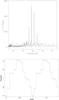 |
Fig. 1 Top: Lomb-Scargle periodogram obtained from the INTEGRAL 22−40 keV lightcurve. Bottom: INTEGRAL lightcurve folded with a period of 9.742 days. |
3.2. Pulse arrival times
Pulse arrival times (PATs, hereafter) were obtained from the broad-band 0.2−10 keV lightcurves obtained by XMM-Newton. Close to the eclipse (φ = 0.03, 0.08, 0.91, 0.01), when the compact object is behind the massive star, pulses could not be detected. We did not extract PATs for the observation of 2004.
To determine the PATs, we used a pulse profile template. This template is derived by folding the lightcurve from observation 0405640801 with a period of 414.2 s, obtained using the Lomb-Scargle technique (Press & Rybicki 1989). This observation was selected because the source was very bright for a long and almost uninterrupted exposure.
A sequence of pulse profile template was fit to each individual lightcurve. This sequence is characterized by: (i) the time of a pulse at the middle of the observation; (ii) the pulse period; and (iii) the amplitudes of each pulse. This assumes that the pulse period is reasonably constant during each observation.
The statistical errors in the pulse time and period are typically 0.01 s and 0.1 s, respectively. Table 2 lists the pulse times and the pulse period obtained at the middle of each observation.
The PAT accuracy is limited by the systematic error related to the assumed pulse profile template. Using a different pulse profile template (derived from observation 0405640901) produces PAT with an offset between 8 s and 12 s from the values listed in Table 2. We adopted a systematic error of 10 s.
Pulse arrival times and derived pulse period.
3.3. Orbital solution
We derived the orbital solution using the PATs of the RXTE observation obtained by Thompson et al. (2007, Epoch 3, see Fig. 2, and the PATs derived above from XMM data.
The orbital solution was obtained by comparing the observed pulse arrival delays (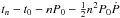 ) to the expected ones αxsini cos [2π(tn − T90)/Porb] (Levine et al. 2004). The orbital parameters (the orbital period, Porb; the projected semi-major axis, αxsini; the reference time corresponding to mid-eclipse, T90) were assumed to be constant. To account for pulse evolution, two sets of pulse parameters (spin period at time t0, P0; spin period derivative, Ṗ) were used for the RXTE and XMM campaigns. The pulse number n was given by the nearest integer to n = (tn − t0)/(P0 + 0.5Ṗ(tn − t0)).
We performed a combined fit of the RXTE and XMM observations. We derived the orbital solutions by (i) allowing all parameters to vary freely and (ii) fixing the orbital period to the value derived from the INTEGRAL data. The resulting parameters are listed in Table 3. We were also able to obtain an upper limit (90%) of e < 0.15 on the eccentricity by adding the first-order term in a Taylor series expansion in the eccentricity (Levine et al. 2004). The RXTE and XMM orbital solutions are comparable and the resulting parameters are consistent within the errors.
The folded lightcurve obtained with the INTEGRAL derived orbital period (Fig. 1, lower panel) results in a pulse fraction ~100%. For the rest of the analysis, we used the orbital solution obtained with fixed Porb (Table 3).
Figure 2 shows the resulting pulse arrival-time delays (fixed Porb) for both RXTE and XMM data together with the best-fit orbital solution.
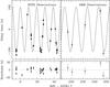 |
Fig. 2 Delays (top) and residuals (bottom) derived from the fixed Porb orbital solution compared to the data. Left: RXTE data are taken from Thompson et al. (2007). Right: XMM − Newton data from this work. |
Orbital solution for IGR J17252–3616.
4. Spectral analysis
The spectral analysis was performed using the XSPEC4 package version 11.3.2ag (Arnaud 1996). To use the  statistics, we grouped the data to have at least 25 (faint spectra) and up to 100 (bright spectra) counts per bin. We initially fitted the observed spectra using a phenomenological model made of an intrinsically absorbed cutoff power-law, a blackbody soft excess, and a gaussian Fe Kα line (wabs*(bb+gauss+vphabs*cutoff)). The centroid of the iron line is compatible with Ec ~ 6.40 ± 0.03 keV at all epochs.
The spectra are always strongly absorbed below ~3 keV and display an iron K-edge at ~7.2 ± 0.2 keV. We first fit each spectrum by assuming all parameters to be free, apart from the Galactic absorption, which was fixed to NH = 1.5 × 1022 cm-2 (Dickey & Lockman 1990).
Some parameters (photon index, cutoff energy, blackbody temperature, and absorber Fe metallicity) did not vary (within the 90% errors) among the observations and were fixed to their average values of EC = 8.2 keV, Γ = 0.02, and kTBB = 0.5 keV, Z = 1 Z⊙. The Fe line was fixed to an energy of 6.4 keV, with a narrow width. Two representative spectra are displayed in Fig. 3.
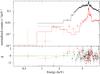 |
Fig. 3 Top: folded model and data for φ = 0.65 (black) and φ = 0.91 (red). Bottom: the corresponding residuals using the model described in the text with the parameters from Table 4. |
The intrinsic absorbing column density and the normalization of each component were allowed to vary freely. The best-fit model parameters are listed in Table 4. Figure 4 shows the variation in all these parameters and in both the unabsorbed 2−10 keV flux and Fe Kα equivalent width (EW). The unabsorbed Fe Kα EW was calculated by setting the intrinsic absorbing column density to zero. All the spectral fits were good resulting in  , apart from the φ = 0.03 observation for which a poor fit was obtained. For the observations made during the eclipse, some parameters are poorly constrained.
Spectral analysis results.
The unabsorbed continuum flux (Fig. 4f) is on the order of ~5 × 10-11 erg cm-2 s-1 outside the eclipse. Variations are observed across the range (2−10) × 10-11 erg cm-2 s-1 and can be interpreted as variations in the accretion rate (Ṁ). During the eclipse, the continuum flux drops by a factor of ~200 and remains stable at the level of  10-13 erg cm-2 s-1.
The intrinsic absorbing column density (Fig. 4b) is persistently high (≳1023 cm-2). Significant variations are detected for φ = 0.2−0.4 and close to the eclipse, reaching values of NH ~ 9 × 1023 cm-2.
The normalization of the blackbody component (Fig. 4c) does not show any variability, although the low energy part of the spectrum is poorly constrained. The normalization of the blackbody component is compatible with ~1033 erg s-1 assuming a distance of 8 kpc. The very high intrinsic absorbing column density rules out the neutron star as the origin of the soft excess.
The flux and EW of the Fe Kα line are displayed in Figs. 4d and 4e, respectively. Both components display significant variations indicating that the region emitting the line is at least partially obscured by the mass-donor star.
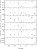 |
Fig. 4 Spectral variability along the orbit illustrated by a) the cut-off power-law normalization at 1 keV, b) the intrinsic hydrogen column density, c) the soft excess blackbody luminosity, assuming a distance of 8 kpc, d) the iron line flux, e) the iron line equivalent width calculated for the unabsorbed continuum, and f) the unabsorbed flux. Dashed vertical lines indicate the eclipse boundary. |
As the X-ray continuum illuminating the gas emitting the Fe fluorescent line cannot be measured during the eclipse, we calculated a corrected Fe Kα EW by assuming a constant continuum flux of 1.8 × 10⁻³ ph keV-1 cm-2 s-1 (Table 4).
5. Discussion
5.1. Constraining the physical parameters of the system
In the previous sections, we have derived an orbital solution (Table 3) yielding a mass function  ± 0.7 M⊙. This is consistent with a high mass X-ray binary system.
Adopting an inclination i = 90°, we infer a mass MOB ~ 14 M⊙ for the donor star. Radial velocity observations showed that q = MX/MOB ~ 0.1 (Mason et al. 2010). Using an upper limit on the mass of ~20 M⊙ (Thompson et al. 2007) constrains the inclination of the orbit i > 70°. Mason et al. (2010) estimated an inclination i ≈ 75°−90°. Within this range, the mass of the donor star is constrained to be MOB ≈ 14−17 M⊙. The mass ratio and the donor mass imply a neutron star mass of MNS = 1.4−1.7 M⊙. The masses of both the donor star and the compact object are roughly similar (within a factor of 2) to that of Vela X-1 (Quaintrell et al. 2003; van Kerkwijk et al. 1995).
The separation of the system could be derived from the duration of the eclipse and the inclination (Joss & Rappaport 1984). For the eclipse duration of Δφ ≈ 0.18 ± 0.02 (i.e. 1.75 days), we can estimate the separation to be αx ≈ 1.7−1.8 R∗. The Roche lobe of the system is RL = 0.99−1.06 R∗ assuming a synchronous rotation (Joss & Rappaport 1984). This means that the system is very close to filling its Roche lobe and to forming an accretion disk, although no significant spin-up has been observed.
Using our VLT observations, Mason et al. (2009) performed near-IR spectroscopy of IGR J17252–3616 and concluded that the donor star is between B0−B5 I and B0−B1 Ia with an effective temperature Teff = 22−28 kT and a stellar radius of R∗ = 22−36 R⊙. On the basis of this spectroscopic determination, we obtain absolute numbers for the separation (αx ≈ 37−64 R⊙) and the Roche lobe radius (RL ≈ 22−38 R⊙).
The unabsorbed 2−10 keV source flux is in the range (0.2−1.3) × 10-10 erg s-1 cm-2. Adopting a mean value of (0.8 ± 0.3) × 1010 erg s-1 cm-2 and assuming a distance of 8 kpc (Mason et al. 2009), the inferred 2−10 keV unabsorbed luminosity is LX ~ 1036 erg s-1. Assuming accretion as the source of energy (where LX = ϵṀc2), we can estimate a mass accretion rate of Ṁ ~ 10-9 M⊙ yr-1, which is similar to that of Vela X-1 (Fürst et al. 2010).
During the eclipse, the X-ray luminosity drops by a factor of ~200 resulting in LX ~ 5 × 1033 erg s-1. As OB stars emit in X-rays with a luminosity LX ~ 1031−32 erg s-1 (Güdel & Nazé 2009), this emission is probably dominated by X-ray scattering in the stellar wind (Haberl 1991). Hickox et al. (2004) discussed the origins of the soft X-ray excesses of many types of accreting pulsars. It is likely that the fairly constant soft X-ray excess observed in IGR J17252–3616 is emitted by recombination lines (Schulz et al. 2002) in a region of the wind larger than the stellar radius (Watanabe et al. 2006).
For a spherically symmetric stellar wind, one would expect to have smooth and predictable variations in the absorbing column density along the orbit. In particular, observations along the same line of sight or symmetric when compared to the eclipse must result in different, respectively identical, column densities. Our observing strategy resulted in NH(φ = 0.15) ≈ NH(φ = 0.37), NH(φ = −0.35) > NH(φ = 0.37) and NH(φ = −0.35) ≈ NH(φ = −0.21), ruling out a spherical geometry.
5.2. Stellar wind structure
We constructed a 3D model of the OB supergiant stellar wind to simulate the variability of the intrinsic column density (NH) and the Fe Kα line equivalent width (EW), during the orbit, and compare them with the observations. We assumed a distance D ≈ 8 kpc (Mason et al. 2009), a circular orbit (e = 0), and an edge-on geometry (i = 90°).
Variability of absorption along the orbit
We first investigated the behavior of the intrinsic column density, NH, as a function of phase, to identify the structure of the wind during the orbit. We approximated the wind structure with two components, the unperturbed wind (ρwind) and a tail-like hydrodynamic perturbation (ρtail) related to the presence of the neutron star. Tail-like structures are expected for the photoionization and heating of the wind leading to strong shock formation and dense sheets of gas trailing the neutron star (Fransson & Fabian 1980). These shocks are produced by hydrodynamical simulations (Blondin et al. 1990) but produce a NH of up to ~1022 cm-2, which is too small to account for the variability observed in IGR J17252–3616.
The unperturbed stellar wind was modeled by assuming a standard wind profile (Castor et al. 1975) 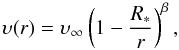 where υ(r) is the wind velocity at distance r from the stellar center, υ∞ is the terminal velocity of the wind, and β is a parameter describing the wind gradient. The conservation of mass provides the radial density distribution of the stellar wind. The unperturbed stellar wind is a good approximation within the orbit of the neutron star. Hydrodynamical simulations (Blondin et al. 1990, 1991; Blondin 1994; Blondin & Woo 1995; Mauche et al. 2008) of HMXB have shown that the wind can be highly disrupted by the neutron star beyond the orbit.
To estimate the terminal velocity of the unperturbed wind, we studied the NH variability using three different sets of parameters (Fig. 5). The mass-loss rate and terminal velocity are constrained by the data to be in the range Ṁw/υ∞ ~ (0.7−2) × 10-16 M⊙/km (β has a very limited impact on the results, so we used 0.7).
The fraction of the wind captured by the neutron star could be estimated from the accretion radius  × 1011 cm (where υorb = 250 km s-1 is the orbital velocity) as
 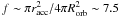 × 10-4. The mass-loss rate is therefore Ṁw ~ f-1Ṁ ≈ 1.5 × 10⁻⁶ M⊙/yr and the terminal velocity of the wind is constrained to be in the interval υ∞ ~ 250−600 km/h.
In our simulation, we adopted a terminal velocity υ∞ = 400 km s-1, a stellar radius R∗ = 29 R⊙, a wind gradient β = 0.7, and a mass loss rate  = 1.35 × 10⁻⁶ M⊙ yr-1. The assumed, observed, and inferred model parameters are listed in Table 5. The variability of NH along the orbit indicates that the unperturbed wind is adequate for phases φ ≈ 0−0.35. For φ ≳ 0.35, NH increases at a value of ~2 × 1023 cm-2. This indicates that a high density tail-like structure lies on one side of the orbit, trailing the neutron star. The tail-like component is still present up to φ ≳ 0.8.
We assumed that the tail-like structure is created very close to the neutron star and opens up with distance. The density of the material inside the “tail” decreases with distance to ensure mass conservation. Its distribution follows a “horn”-like shape with a circular section. We adjusted the density of the tail-like structure to match the observations. The density distribution ρwind + ρtail is displayed in Fig. 6. The supergiant is located at the center (black disk). The tail-like structure covers about half of the orbit.
Figure 5 displays the simulated NH variability from the above density distribution together with the observed data points. The data and the model shows that the tail-like perturbation is essential to understand the observed variations.
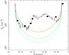 |
Fig. 5 Simulated NH variations plotted together with the data. We illustrate three different smooth wind configurations, for Ṁ/υ∞ = 0.7 (cyan), 1 (green), and 2 (red) × 10-16 M⊙/km, keeping all the other parameters fixed. The solid black line shows the total NH consisting of the unperturbed stellar wind (green line) and the tail-like extended component. The observations during the eclipse have been omitted. |
Wind model parameters.
Variability of the Fe Kα line during the orbit
Assuming that the intrinsic X-ray flux is unaffected by the eclipse, the Fe Kα equivalent width drops by a factor of ~10 during the eclipse in an orbital phase interval of ~0.1. This indicates that the radius of the region emitting Fe Kα is smaller than half of the stellar radius (<1012 cm) and far more compact than the tail structure responsible for the absorption variability profile.
Vela X-1 shows a similar behavior, which was interpreted as an emitting region of the size of (Ohashi et al. 1984), or even within (Endo et al. 2002) the accretion radius.
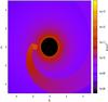 |
Fig. 6 Number density distribution in the plane of the orbit including a smooth wind and a tail-like perturbation. The black disk at the center represents the supergiant star. |
Outside the eclipse, the equivalent width of the Fe Kα line is of the order of 100 eV. Following Matt (2002) and assuming a spherical transmission geometry, this corresponds to a column density of NH ~ 2 × 1023 cm-2. As this additional absorption is not observed, the region emitting Fe Kα must be partially ionized.
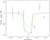 |
Fig. 7 Corrected unabsorbed Fe Kα line equivalent width along the orbit. Green curve indicates the prediction of the hydrodynamical tail and the black curve the addition of the central cocoon. |
An ionization parameter ξ = L/nR2 in the range 10−300 is required to fully ionize light elements contributing to the soft X-ray absorption and keep an Fe Kα line at the energy of 6.4 keV (Kallman et al. 2004; Kallman & McCray 1982). The density of the Fe Kα emitting region is therefore ~ξ-1R12-2 × 1012 cm-3, where R12 is the distance from the neutron star in units of 1012 cm. As NH = nR ~ 2 × 1023 cm-2, we have ξ ~ 5/R12. A dense cocoon is therefore needed around the neutron star with a size 0.5 > R12 > 0.02 and a density 1011 cm-3 < n < 3 × 1012 cm-3.
The majority of the Fe Kα is formed in a region that is small enough to allow for pulsation of the Fe Kα line, as observed in Cen X–3 (Day et al. 1993) and Her X–1 (Choi et al. 1994). We searched for such pulsations in our longest and almost uninterrupted observation (obsID 0405640801; φ = 0.40). Folded lightcurves were built in the energy bands 6.2−6.7 keV, 2−6.1 keV, and 6.8−10 keV and resulted in a pulse fraction of 49 ± 5%, 58 ± 3%, and 57 ± 4%, respectively. The ratio of the line flux to the continuum in the energy range 6.2−6.7 keV is ~0.25. Assuming that the line is not pulsed, we infer an Fe Kα pulse fraction of ~50%, which is in good agreement with the above measurement. Weak Fe Kα pulsation can be explained if the cocoon is isotropic.
To match the observed column density variability, the radius and the density of the inner region of the tail structure were set to 4 × 1011 cm and 3 × 1011 cm-3, respectively. It is therefore very likely that the dense cocoon corresponds to the inner and ionized region of the hydrodynamical tail. We thus added this partially ionized cocoon in our simulations, using a density of 3 × 1011 cm-3 within a radius of ~6 × 1011 cm ~ 3 Racc. The Fe Kα emissivity map (Fig. 8) was calculated by applying an illuminating radiation field (~1/r2) to the density distribution. Figure 7 displays the resulting simulated profile of the Fe Kα equivalent width together with the observed data. The green curve shows the variations in the Fe Kα equivalent width expected from the wind density profile excluding the central cocoon, which obviously could not reproduce the data. The black curve accounts for the dense central cocoon. The exact profile of the eclipse is related to the size and density profile of the cocoon. No effort has been made to obtain an exact match to the data.
The ionized cocoon is expected to produce an iron K-edge at ~7.8 keV. For a column density of NH ~ 2 × 1023 cm-1, its optical depth τ ~ 0.2 (Kallman et al. 2004) remains difficult to detect. Even our observation at an orbital phase 0.15 (the best candidate for the detection of the ionised edge) does not have enough signal.
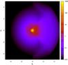 |
Fig. 8 Integrated Fe Kα emissivity (relative units) centered on the neutron star at phase φ = 0.5. The smooth circular halo shows the rim of the supergiant star. The tail structure can be observed on the right. |
The mass of the tail-like structure Mtail ~ 10-8 M⊙ can be accumulated in ttail = Mtail/Ṁ, where  and reff is an effective radius for the funneling of the wind in the tail. For a tail accumulation timescale (ttail) comparable to the orbital period of (~10 days), this effective radius is 12 Racc.
The orientation of the tail-like structure depends on the wind and orbital velocities. The angle between the wind velocity and the orbital velocity is given by tan(α) = υorb/υ. The tail obtained in our simulations is tilted by α ~ 80°. This corresponds to υ ~ 0.2 υorb ≈ 50 km s-1, which is lower than υ(Rorb) ≈ 250 km s-1 because of the ionization of the stellar wind in the vicinity of the neutron star.
6. Conclusions
We have presented the analysis of an observing campaign performed with XMM-Newton on the persistently absorbed sgHMXB IGR J17252–3616. Nine observations have been performed over about four weeks, distributed across various orbital phases. Three of them were scheduled during the eclipse of the neutron star by the companion star.
We first refined the orbital solution, using in addition archival INTEGRAL and RXTE data and found an orbital period of 9.742 d and a projected orbital radius of 101 ± 2 lt-s. The pulsar spin period varies between 414.3 and 413.8 s during the observing campaign.
The X-ray spectrum (0.2–10 keV), which varies during the orbit, was successfully fitted using an absorbed cut-off power-law continuum, a soft excess, and a gaussian emission line. The soft excess, modeled with a black body, remained constant.
The continuum component varies in intensity (a measure of the instantaneous accretion rate) but displays a constant spectral shape, as usually observed in accreting pulsars.
The absorbing column density and the Fe Kα emission line show remarkable variations. The column density, always above 1023 cm-2, increases towards 1024 cm-2 close to the eclipse, as expected for a spherically symmetric wind. The wind velocity is unusually small close to υ∞ = 400 km s-1. An additional excess of absorption of 2 × 1023 cm-2 is observed for orbital phases φ > 0.3, which is found to represent a hydrodynamical tail trailing the neutron star.
During the eclipse, the equivalent width of the Fe Kα line drops by a factor >10 indicating that most of the line is emitted in a cocoon surrounding the pulsar, with a size of a few accretion radii. This cocoon is ionized and corresponds to the inner region of the hydrodynamical tail.
The parameters of the IGR J17252–3616 are very similar to these of Vela X-1, except for the smaller wind velocity. We argue that the persistently large absorption column density is related to the hydrodynamical tail, which has been strengthened by the low wind velocity. The tail is a persistent structure dissolving on a timescale comparable to the orbital period.
Our interpretation can be tested using numerical hydrodynamical simulations and high resolution optical/infrared spectroscopy. If confirmed, it may turn out that half of the persistent sgHMXB have stellar wind speeds several times lower than usually measured.
References
- Arnaud, K. A. 1996, in Astronomical Data Analysis Software and Systems V, ed. G. H. Jacoby, & J. Barnes, ASP Conf. Ser., 101, 17 [Google Scholar]
- Blondin, J. M. 1994, ApJ, 435, 756 [NASA ADS] [CrossRef] [EDP Sciences] [Google Scholar]
- Blondin, J. M., & Woo, J. W. 1995, ApJ, 445, 889 [NASA ADS] [CrossRef] [Google Scholar]
- Blondin, J. M., Kallman, T. R., Fryxell, B. A., & Taam, R. E. 1990, ApJ, 356, 591 [NASA ADS] [CrossRef] [Google Scholar]
- Blondin, J. M., Stevens, I. R., & Kallman, T. R. 1991, ApJ, 371, 684 [NASA ADS] [CrossRef] [Google Scholar]
- Castor, J. I., Abbott, D. C., & Klein, R. I. 1975, ApJ, 195, 157 [NASA ADS] [CrossRef] [Google Scholar]
- Charles, P. A., & Coe, M. J. 2006, Optical, ultraviolet and infrared observations of X-ray binaries, ed. W. H. G. Lewin, & M. van der Klis, 215 [Google Scholar]
- Chaty, S., Rahoui, F., Foellmi, C., et al. 2008, A&A, 484, 783 [NASA ADS] [CrossRef] [EDP Sciences] [Google Scholar]
- Choi, C. S., Nagase, F., Makino, F., et al. 1994, ApJ, 437, 449 [NASA ADS] [CrossRef] [Google Scholar]
- Corbet, R. H. D. 1986, MNRAS, 220, 1047 [NASA ADS] [CrossRef] [Google Scholar]
- Day, C. S. R., Nagase, F., Asai, K., & Takeshima, T. 1993, ApJ, 408, 656 [NASA ADS] [CrossRef] [Google Scholar]
- Dickey, J. M., & Lockman, F. J. 1990, ARA&A, 28, 215 [NASA ADS] [CrossRef] [MathSciNet] [Google Scholar]
- Endo, T., Ishida, M., Masai, K., et al. 2002, ApJ, 574, 879 [NASA ADS] [CrossRef] [Google Scholar]
- Fransson, C., & Fabian, A. C. 1980, A&A, 87, 102 [NASA ADS] [Google Scholar]
- Fürst, F., Kreykenbohm, I., Pottschmidt, K., et al. 2010, A&A, 519, A37 [NASA ADS] [CrossRef] [EDP Sciences] [Google Scholar]
- Güdel, M., & Nazé, Y. 2009, A&ARv, 17, 309 [NASA ADS] [CrossRef] [Google Scholar]
- Haberl, F. 1991, A&A, 252, 272 [NASA ADS] [Google Scholar]
- Hickox, R. C., Narayan, R., & Kallman, T. R. 2004, ApJ, 614, 881 [NASA ADS] [CrossRef] [Google Scholar]
- Jansen, F., Lumb, D., Altieri, B., et al. 2001, A&A, 365, L1 [NASA ADS] [CrossRef] [EDP Sciences] [Google Scholar]
- Joss, P. C., & Rappaport, S. A. 1984, ARA&A, 22, 537 [NASA ADS] [CrossRef] [Google Scholar]
- Kallman, T. R., & McCray, R. 1982, ApJS, 50, 263 [NASA ADS] [CrossRef] [Google Scholar]
- Kallman, T. R., Palmeri, P., Bautista, M. A., Mendoza, C., & Krolik, J. H. 2004, ApJS, 155, 675 [NASA ADS] [CrossRef] [Google Scholar]
- Lebrun, F., Leray, J. P., Lavocat, P., et al. 2003, A&A, 411, L141 [NASA ADS] [CrossRef] [EDP Sciences] [Google Scholar]
- Levine, A. M., Rappaport, S., Remillard, R., & Savcheva, A. 2004, ApJ, 617, 1284 [NASA ADS] [CrossRef] [Google Scholar]
- Liu, Q. Z., van Paradijs, J., & van den Heuvel, E. P. J. 2006, A&A, 455, 1165 [NASA ADS] [CrossRef] [EDP Sciences] [Google Scholar]
- Mason, A. B., Clark, J. S., Norton, A. J., Negueruela, I., & Roche, P. 2009, A&A, 505, 281 [NASA ADS] [CrossRef] [EDP Sciences] [Google Scholar]
- Mason, A. B., Norton, A. J., Clark, J. S., Negueruela, I., & Roche, P. 2010, A&A, 519, A79 [NASA ADS] [CrossRef] [EDP Sciences] [Google Scholar]
- Matt, G. 2002, MNRAS, 337, 147 [NASA ADS] [CrossRef] [Google Scholar]
- Mauche, C. W., Liedahl, D. A., Akiyama, S., & Plewa, T. 2008, in Am. Inst. Phys. Conf. Ser., ed. M. Axelsson, 1054, 3 [Google Scholar]
- Ohashi, T., Inoue, H., Koyama, K., et al. 1984, PASJ, 36, 699 [NASA ADS] [Google Scholar]
- Press, W. H., & Rybicki, G. B. 1989, ApJ, 338, 277 [NASA ADS] [CrossRef] [Google Scholar]
- Quaintrell, H., Norton, A. J., Ash, T. D. C., et al. 2003, A&A, 401, 313 [NASA ADS] [CrossRef] [EDP Sciences] [Google Scholar]
- Rahoui, F., Chaty, S., Lagage, P., & Pantin, E. 2008, A&A, 484, 801 [NASA ADS] [CrossRef] [EDP Sciences] [Google Scholar]
- Schulz, N. S., Canizares, C. R., Lee, J. C., & Sako, M. 2002, ApJ, 564, L21 [NASA ADS] [CrossRef] [Google Scholar]
- Strüder, L., Briel, U., Dennerl, K., et al. 2001, A&A, 365, L18 [NASA ADS] [CrossRef] [EDP Sciences] [Google Scholar]
- Takeuchi, Y., Koyama, K., & Warwick, R. S. 1990, PASJ, 42, 287 [NASA ADS] [Google Scholar]
- Tawara, Y., Yamauchi, S., Awaki, H., et al. 1989, Astron. Soc. Japan, 41, 473 [Google Scholar]
- Thompson, T. W. J., Tomsick, J. A., in ’t Zand, J. J. M., Rothschild, R. E., & Walter, R. 2007, ApJ, 661, 447 [NASA ADS] [CrossRef] [Google Scholar]
- van Kerkwijk, M. H., van Paradijs, J., Zuiderwijk, E. J., et al. 1995, A&A, 303, 483 [NASA ADS] [Google Scholar]
- Walter, R., Bodaghee, A., Barlow, E. J., et al. 2004, The Astronomer’s Telegram, 229, 1 [Google Scholar]
- Walter, R., Zurita Heras, J., Bassani, L., et al. 2006, A&A, 453, 133 [NASA ADS] [CrossRef] [EDP Sciences] [Google Scholar]
- Warwick, R. S., Norton, A. J., Turner, M. J. L., Watson, M. G., & Willingale, R. 1988, MNRAS, 232, 551 [NASA ADS] [CrossRef] [Google Scholar]
- Watanabe, S., Sako, M., Ishida, M., et al. 2006, ApJ, 651, 421 [NASA ADS] [CrossRef] [Google Scholar]
- White, N. E. 1989, A&ARv, 1, 85 [NASA ADS] [Google Scholar]
- White, N. E., Nagase, F., & Parmar, A. N. 1995, in X-ray Binaries, ed. W. H. G. Lewin, J. van Paradijs, & E. P. J. van den Heuvel, 1 [Google Scholar]
- Winkler, C., Courvoisier, T., Di Cocco, G., et al. 2003, A&A, 411, L1 [NASA ADS] [CrossRef] [EDP Sciences] [Google Scholar]
- Zurita Heras, J. A., de Cesare, G., Walter, R., et al. 2006, A&A, 448, 261 [NASA ADS] [CrossRef] [EDP Sciences] [Google Scholar]
All Tables
All Figures
|
Fig. 1 Top: Lomb-Scargle periodogram obtained from the INTEGRAL 22−40 keV lightcurve. Bottom: INTEGRAL lightcurve folded with a period of 9.742 days. |
| In the text | |
|
Fig. 2 Delays (top) and residuals (bottom) derived from the fixed Porb orbital solution compared to the data. Left: RXTE data are taken from Thompson et al. (2007). Right: XMM − Newton data from this work. |
| In the text | |
|
Fig. 3 Top: folded model and data for φ = 0.65 (black) and φ = 0.91 (red). Bottom: the corresponding residuals using the model described in the text with the parameters from Table 4. |
| In the text | |
|
Fig. 4 Spectral variability along the orbit illustrated by a) the cut-off power-law normalization at 1 keV, b) the intrinsic hydrogen column density, c) the soft excess blackbody luminosity, assuming a distance of 8 kpc, d) the iron line flux, e) the iron line equivalent width calculated for the unabsorbed continuum, and f) the unabsorbed flux. Dashed vertical lines indicate the eclipse boundary. |
| In the text | |
|
Fig. 5 Simulated NH variations plotted together with the data. We illustrate three different smooth wind configurations, for Ṁ/υ∞ = 0.7 (cyan), 1 (green), and 2 (red) × 10-16 M⊙/km, keeping all the other parameters fixed. The solid black line shows the total NH consisting of the unperturbed stellar wind (green line) and the tail-like extended component. The observations during the eclipse have been omitted. |
| In the text | |
|
Fig. 6 Number density distribution in the plane of the orbit including a smooth wind and a tail-like perturbation. The black disk at the center represents the supergiant star. |
| In the text | |
|
Fig. 7 Corrected unabsorbed Fe Kα line equivalent width along the orbit. Green curve indicates the prediction of the hydrodynamical tail and the black curve the addition of the central cocoon. |
| In the text | |
|
Fig. 8 Integrated Fe Kα emissivity (relative units) centered on the neutron star at phase φ = 0.5. The smooth circular halo shows the rim of the supergiant star. The tail structure can be observed on the right. |
| In the text | |
Current usage metrics show cumulative count of Article Views (full-text article views including HTML views, PDF and ePub downloads, according to the available data) and Abstracts Views on Vision4Press platform.
Data correspond to usage on the plateform after 2015. The current usage metrics is available 48-96 hours after online publication and is updated daily on week days.
Initial download of the metrics may take a while.