| Issue |
A&A
Volume 526, February 2011
|
|
|---|---|---|
| Article Number | A157 | |
| Number of page(s) | 4 | |
| Section | Stellar structure and evolution | |
| DOI | https://doi.org/10.1051/0004-6361/201015128 | |
| Published online | 14 January 2011 | |
Peculiar rotation in evolved binary systems: stellar and tidal evolution of TZ Fornacis
Instituto de Astrofísica de Andalucía,
CSIC, Apartado 3004,
18080
Granada,
Spain
e-mail: This email address is being protected from spambots. You need JavaScript enabled to view it.
Received:
1
June
2010
Accepted:
8
September
2010
Abstract
Aims. TZ Fornacis is an evolved binary system with an orbital period of 75.7 days and a circular orbit. The two stars have similar masses (2.045 ± 0.055 and 1.945 ± 0.027 M⊙) but very different radii: 8.33 ± 0.12 and 3.966 ± 0.088 R⊙. One of its most interesting characteristics is that while the primary rotates synchronously with the mean orbital angular velocity, the secondary is rotating 16 times faster than this reference value. The stellar and tidal evolution of such a system was investigated in the past using some simplifications: integration of the time scales for circularization and synchronization that are valid only for low eccentricities and small departures from the synchronism, which are not fully valid for the case of TZ Fornacis. Another detected problem is the inconsistency between the observed levels of circularization/synchronization and the theoretical critical times and the inferred age (the time of synchronization of the secondary was found to be shorter than its age). The main goal of the present paper is to advance a little more in our understanding of the stellar and tidal evolution of TZ For.
Methods. In order to improve our understanding of the tidal evolution of TZ For, we adopt new absolute dimensions and compute specific stellar evolutionary models for the precise observed masses. We explicitly integrate the differential equations that govern the tidal evolution (eccentricity, angular velocities and orbital period) by using these stellar models.
Results. The stellar models indicate that there are two possibilities for the position of the primary on the HR diagram: case A (primary on the clump) and case B (primary on the first ascendent branch). The integration of the complete differential equations of tidal evolution was crucial to shed some light on the tidal evolution of TZ For. The observed levels of circularization/synchronization are now compatible with the inferred age and with the times of circularization/synchronization in both cases. The mentioned inconsistency is no longer detected. In particular, we have found that the primary is synchronized with the orbital period, while the secondary is rotating 17.6 (or 16.2) times faster depending on the selected model, which agrees well with the observations.
Key words: stars: evolution / stars: interiors / binaries: eclipsing / stars: rotation / binaries: general
© ESO, 2011
1. Introduction
The scenario of tidal evolution is not perfectly clear from the theoretical point of view because the comparison with observations presents some disagreement (see Claret & Cunha 1997, for a brief review). Summarising, the hydrodynamical mechanism seems to be too efficient to circularize the orbits, while the predictions by the tidal torque process indicated a lower efficiency than that required to fit the observations. In spite of these problems the tidal evolution theories can be used to infer interesting features of double star systems. If the system in question has a good determination of its relevant astrophysical parameters and presents similar masses, it becomes a very important tool to test the stellar and tidal evolution theories. Both components evolve very similarly during the main-sequence, and small differences in radii and effective temperatures can be detected observationally. However, in the fastest stages of the evolution, significant changes in the astrophysical parameters – mainly radii – are expected to occur. These changes do not only affect the differential stellar evolution, but also the tidal evolution and in consequence, the dynamics of the system.
Of particular importance within this context is that we have evolved systems presenting circular orbits but with asynchronous components. About 15 years ago we have investigated the case of TZ For (Claret & Giménez 1995). The absolute dimensions of that system were recently published by Torres et al. (2010) and they are based on the paper by Andersen et al. (1991). The masses of the primary and the secondary are similar (2.045 ± 0.055 and 1.945 ± 0.027 M⊙), but the radii are very different: 8.33 ± 0.12 and 3.966 ± 0.088 R⊙. The orbital period is 75.7 days. The primary star is rotating synchronously with the orbital period, but the secondary rotates about 16 times faster than the synchronous value. The asynchronysm of the secondary component could be explained in the mentioned paper by significant changes in the moment of inertia during a short time interval (Claret & Giménez 1995). However, there are two points in that paper that require some revision. First, we have integrated the time scales for circularization and synchronization, which are valid only for low eccentricities and small departures from the synchronism (for the definition of tcir and tsync12 see for example Claret & Giménez 1995; Claret & Cunha 1997). While the first condition can be considered as marginally acceptable at least for the present but not necessarily in the past, the second one is clearly in contradiction with the asynchronism of the secondary. Second, the critical times for circularization and synchronization we have found were not fully compatible with the observations although they are on the same order of the evolutionary age (log t = 9.11). The critical time for circularization (log tcir = 9.05) is compatible with the observed eccentricity and age. The same holds for the primary, which is synchronized at log tsync1 = 9.00. However, for the secondary the situation is different. Indeed, given the observed level of synchronization of the secondary, its critical time for synchronism (log tsync2 = 9.03) is not consistent with the inferred age.
The principal goal of the present paper is to try to advance a little more in the understanding of the stellar and tidal evolution of TZ For. To do that, we adopt the revised absolute dimensions and compute specific stellar evolutionary models and integrate explicitly the differential equations that govern the tidal evolution (eccentricity, angular velocities and orbital period). In Sect. 2 we describe the stellar models and present the tidal evolution equations. Then we apply the computations to the case of TZ For and finally we present our results and conclusions.
2. Stellar models for TZ For and the equations of the tidal evolution
The stellar models were generated with the Granada evolutionary code by Claret (2004). We considered core overshooting described as an extra mixing beyond the classical Schwarzschild criterion. For the excess distance we use dover = αovHp, where Hp is the pressure scale height taken at the edge of the convective core as given by Schwarzschild’s criterion and αov is a free parameter. The dependence of αov with stellar mass was considered following the results by Claret (2007). For models with convective envelopes, we adopted the mixing-length theory to describe them, with α = 1.68, as calibrated using the Sun.
For high temperatures the code uses the set of tables provided by Iglesias & Rogers (1996), completed with the computations by Alexander & Ferguson (1994) for lower temperatures. Mass loss was considered during the Main-Sequence and for red giants. Given the evolutionary status and the masses of TZ For, the formalism by Nieuwenhuijzen & de Jager (1990) was considered for all models, and for the red giants stage we adopted the formalism by Reimers (1977).
There are several attempts to fit the astrophysical parameters of TZ For. For example,
Lastennet & Valls-Gabaud (2002) used other
stellar evolution codes, but they were unable to reproduce the astrophysical parameters of
TZ For at the same isochrone. Similar results were obtained by other authors (Young
& Arnett 2005; VandenBerg et al. 2006). We obtain an acceptable fit with the primary in
the clump by assuming (X,Z) = (0.016,0.72). However, as in the case of the
mentioned attempts, the error bars in the inferred age are relatively large and we do not
consider these models here. Such a difficulty – to reproduce the observed parameters for TZ
For – may be related to deficiencies in stellar modeling in the later phases of evolution.
Another deficiency may be related to the absolute effective temperatures. These parameters
are highly dependent on calibration, distance and models of stellar atmospheres. In order to
avoid possible complications with the effective temperature calibrations we use the R-log
(age) plane. We have considered two possibilities for the position of the primary on the HR
diagram. In the first one we consider the primary in the helium-burning phase (Fig. 1) (see also Claret & Giménez 1995; Lastennet & Valls-Gabaud 2002). The adopted chemical composition was (X,Z) = (0.730,0.010)
and αov = 0.20. This chemical composition has an additional
point of uncertainty because of the discussion about the value of the metallicity of the Sun
(Basu 2008). The vertical lines in Fig. 1 denote the ages of each component and an average common
age of  is
obtained. When the error bars in the observed masses are considered, the error bars in the
age increase and the result is
is
obtained. When the error bars in the observed masses are considered, the error bars in the
age increase and the result is  .
In the second solution, the primary is on the first ascendent branch (see also Young
& Arnett 2005; and VandenBerg et al. 2006). A common age of
.
In the second solution, the primary is on the first ascendent branch (see also Young
& Arnett 2005; and VandenBerg et al. 2006). A common age of
 was found for (X,Z) = (0.706,0.018) and
αov = 0.50, a value already found in Claret (2007). The more probable likely case is case A because the
primary is in a relatively slow phase, while in case B such a star is evolving very rapidly
and therefore it is less probable under the statistical point of view.
was found for (X,Z) = (0.706,0.018) and
αov = 0.50, a value already found in Claret (2007). The more probable likely case is case A because the
primary is in a relatively slow phase, while in case B such a star is evolving very rapidly
and therefore it is less probable under the statistical point of view.
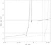 |
Fig. 1 Radius evolution of TZ For (the continuous line represents the primary and the dashed one the secondary). The radius is in solar units, while the time is given in years. The horizontal lines denote the observed radii and their error bars. The vertical dashed lines mark the inferred ages of each component of the system. Case A. |
The differential equations for the tidal evolution in the weak friction model can be
written as (Hut 1981; see also Eggleton &
Kiseleva-Eggleton 2002)
 (3)
(3) (4)where e is
the orbital eccentricity, A is the semimajor axis, Ωi is the
angular velocity of the component i, ω is the mean orbital
angular velocity, βi is the radius of gyration
of the component i, k2i is the apsidal motion
constant of the component i,
Ri is the radius of the component
i,
q = M2/M1,
q2 = M1/M2
and tF is an estimate on the timescale of tidal friction and it
is given by
(4)where e is
the orbital eccentricity, A is the semimajor axis, Ωi is the
angular velocity of the component i, ω is the mean orbital
angular velocity, βi is the radius of gyration
of the component i, k2i is the apsidal motion
constant of the component i,
Ri is the radius of the component
i,
q = M2/M1,
q2 = M1/M2
and tF is an estimate on the timescale of tidal friction and it
is given by  (5)The auxiliary functions
fk can be written as
(5)The auxiliary functions
fk can be written as
 (6)
(6) (7)
(7) (8)
(8) (9)
(9) (10)In order to compute the
theoretical internal structure constants kj
necessary to integrate above the tidal evolution equations, we integrated the described
models using the differential equations of Radau as given by
(10)In order to compute the
theoretical internal structure constants kj
necessary to integrate above the tidal evolution equations, we integrated the described
models using the differential equations of Radau as given by
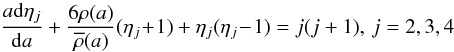 (11)where
 (12)and
a is the mean radius of the configuration ,
ϵj is a measure of the deviation from
sphericity, ρ(a) is the mass density at the distance
a from the center, and
(12)and
a is the mean radius of the configuration ,
ϵj is a measure of the deviation from
sphericity, ρ(a) is the mass density at the distance
a from the center, and  is the mean mass density within a
sphere of radius a. The kj is computed
following the equation
is the mean mass density within a
sphere of radius a. The kj is computed
following the equation 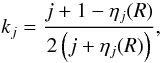 (13)where R
refers the values of ηj at the star’s surface.
(13)where R
refers the values of ηj at the star’s surface.
To integrate the above differential equations we have used the Runge-Kutta fourth order method. The values of the stellar parameters shown in Eqs. (1)–(4) were inferred directly from the respective evolutionary tracks.
3. Discussion of the results and concluding remarks
As we have seen in the previous section, there are two acceptable fittings for TZ For: one with a primary in the clump, during the helium-burning phase (case A) and another one positioning the primary in the first ascendent branch (case B). The differential Eqs. (1)–(4) can be integrated by using these models if we know the initial conditions. Unfortunately this is not the case. However, we can introduce some trial values for the eccentricity, orbital period and angular velocities and investigate how these parameters evolve with time and compare them with the observed levels of circularization and synchronism. This procedure can provide a possible and satisfactory scenario for the tidal evolution of TZ For. We have performed several tests by introducing initial trial values of the eccentricity and angular velocities. The resulting times for circularization are not strongly dependent on the initial eccentricities, but the initial rotational velocities are critical to obtain the correct values of the angular rotation for both components at the inferred age.
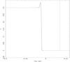 |
Fig. 2 Eccentricity evolution of TZ For. The dashed line indicates the mean age for the system. Case A. |
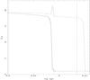 |
Fig. 3 Angular velocity evolution of TZ For. These parameters are normalized to the mean angular orbital velocity. The continuous line represents the primary and the dashed one the secondary. The dashed vertical line indicates the mean age for the system. Case A. |
For case A, we begin with an initial period of 77 days, an initial eccentricity of 0.3 and
assume that both components rotate initially 20 faster than the mean orbital angular
velocity. The initial value for the relative radius of the primary is on the order of 0.01.
This parameter achieves the value 0.24 for more evolved phases when the tidal forces are
more effective. The actual value of the relative radius of the primary is ≈0.07. The
results of the integrations of the tidal equations are shown in Fig. 2 (eccentricity) and Fig. 3 (angular
velocities). The vertical dashed line indicates the mean inferred age. The circularization
is achieved very quickly when the relative radius of the primary is 0.238. The critical time
for circularization is log tcir = 8.991 and is perfectly
consistent with the derived age for TZ For (log t = 9.034) and with the
observed level of circularization. Note that immediatly before the system circularizes the
orbit, there is a small increase in the eccentricity. This is because of the nature of
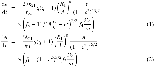
Eq. (1), which governs the eccentricity evolution: depending on the values of the ratio
 we have
de/dt > 0. An interesting feature of the
normalized angular velocities can be seen in Fig. 3.
The synchronism for the primary is achieved more or less at the same time as for
circularization (log tsync1 = 8.990) and reproduces very well
the observed level of synchronism of the primary at the inferred age. Concerning the
secondary, the dashed line shows the evolution of its angular velocity. At the derived age
the models predict that the secondary rotates around 17.6 times faster than the mean orbital
angular velocity, which agrees well with the observed value (16 times). Note that using the
explicit differential equations of tidal evolution the inconsistency pointed out in the
Introduction is solved because all three critical times are compatible with the inferred age
and the synchronism of the secondary is only achieved at log t
around 9.05.
we have
de/dt > 0. An interesting feature of the
normalized angular velocities can be seen in Fig. 3.
The synchronism for the primary is achieved more or less at the same time as for
circularization (log tsync1 = 8.990) and reproduces very well
the observed level of synchronism of the primary at the inferred age. Concerning the
secondary, the dashed line shows the evolution of its angular velocity. At the derived age
the models predict that the secondary rotates around 17.6 times faster than the mean orbital
angular velocity, which agrees well with the observed value (16 times). Note that using the
explicit differential equations of tidal evolution the inconsistency pointed out in the
Introduction is solved because all three critical times are compatible with the inferred age
and the synchronism of the secondary is only achieved at log t
around 9.05.
The tidal evolution in case B is not so different from case A. We have used the same initial parameters as previously. As indicated before, the inferred age is 9.150 and the circularization is achieved at log t = 9.143, which is compatible with the circular orbit of TZ For at the present. On the other hand, the primary should synchronize with the orbital period at about the same time. The evolution of the angular velocity of the secondary is similar to the case A, and at the inferred age, we have Ω1 = 16.2ω, also in very good agreement with the observations. Again the quoted inconsistency between the critical times and age is not detected.
It is remarkable that independently of the evolutionary status of the primary considered (case A or B) the agreement of the observed eccentricity and levels of synchronization of both components with the theoretical predictions is good. Note also that this improvement with respect to the Claret & Giménez (1995) paper is mainly due to the explicit integration of the tidal evolution equations, instead of integrating the timescales. In order to check the capability of our method, we have performed the same calculations of tidal evolution for the models with (X,Z) = (0.016,0.72). The results are very similar to cases A and B – except that the inherent error bars are larger – and the inconsistency mentioned in the Introduction was not detected.
In spite of the good agreement found between the levels of circularization/synchronization and the inferred ages of TZ For,
there is still a limitation in our analysis: the estimate of the timescale of tidal friction. In the present paper we have adopted the value tF = (MR2/L)1/3 which is only a rough approximation for the tidal friction. A more detailed treatment of tF is performed by Eggleton et al. (1998), who give the main ingredients to compute the tidal friction timescale as weighted functions inside each star. These calculations are beyond the scope of the present paper but we hope to present them in a the near future by using TZ For, α Aur and other evolved systems with circular orbits but with asynchronous components.
Acknowledgments
I would like to thank Dr. P. P. Eggleton for useful suggestions that improved the paper. The Spanish MEC (AYA2006-06375, AYA2009-14000-C03-01) is gratefully acknowledged for its support during the development of this work. This research has made use of the SIMBAD database, operated at the CDS, Strasbourg, France, and of NASA’s Astrophysics Data System Abstract Service.
References
- Andersen, J., Clausen, J. V., Nordstrom, B., Tomkin, J., & Mayor, M. 1991, A&A, 246, 99 [NASA ADS] [Google Scholar]
- Alexander, D. R., & Ferguson, J. W. 1994, ApJ, 437, 879 [NASA ADS] [CrossRef] [Google Scholar]
- Basu, S. 2008, ASPC, 384, 10 [NASA ADS] [Google Scholar]
- Claret, A. 2004, A&A, 424, 919 [NASA ADS] [CrossRef] [EDP Sciences] [Google Scholar]
- Claret, A. 2007, A&A, 475, 1019 [NASA ADS] [CrossRef] [EDP Sciences] [Google Scholar]
- Claret, A., & Cunha, N. C. S. 1997, A&A, 318, 187 [NASA ADS] [Google Scholar]
- Claret, A., & Giménez, A. 1995, A&A, 296, 180 [NASA ADS] [Google Scholar]
- Eggleton, P. P., & Kiseleva-Eggleton, L. 2002, ApJ, 575, 461 [NASA ADS] [CrossRef] [Google Scholar]
- Eggleton, P. P., Kiseleva, L. G., & Hut, P. 1998, ApJ, 499, 853 [NASA ADS] [CrossRef] [Google Scholar]
- Hut, P. 1981, A&A, 99, 126 [NASA ADS] [Google Scholar]
- Iglesias, C. A., & Rogers, F. J. 1996, ApJ, 464, 943 [NASA ADS] [CrossRef] [Google Scholar]
- Lastennet, E., & Valls-Gabaud, D. 2002, A&A, 396, 551 [NASA ADS] [CrossRef] [EDP Sciences] [Google Scholar]
- Nieuwenhuijzen, H., & de Jager, C. 1990, A&A, 231, 134 [NASA ADS] [Google Scholar]
- Reimers, D. 1977, A&A, 61, 217 [NASA ADS] [Google Scholar]
- Torres, G., Andersen, J., & Giménez, A. 2010, A&ARv, 18, 67 [Google Scholar]
- VandenBerg, D., Bergbusch, P., & Dowler, P. D. 2006, ApJSS, 162, 387 [Google Scholar]
- Young, P. A., & Arnett, D. 2005, ApJ, 618, 908 [NASA ADS] [CrossRef] [Google Scholar]
All Figures
|
Fig. 1 Radius evolution of TZ For (the continuous line represents the primary and the dashed one the secondary). The radius is in solar units, while the time is given in years. The horizontal lines denote the observed radii and their error bars. The vertical dashed lines mark the inferred ages of each component of the system. Case A. |
| In the text | |
|
Fig. 2 Eccentricity evolution of TZ For. The dashed line indicates the mean age for the system. Case A. |
| In the text | |
|
Fig. 3 Angular velocity evolution of TZ For. These parameters are normalized to the mean angular orbital velocity. The continuous line represents the primary and the dashed one the secondary. The dashed vertical line indicates the mean age for the system. Case A. |
| In the text | |
Current usage metrics show cumulative count of Article Views (full-text article views including HTML views, PDF and ePub downloads, according to the available data) and Abstracts Views on Vision4Press platform.
Data correspond to usage on the plateform after 2015. The current usage metrics is available 48-96 hours after online publication and is updated daily on week days.
Initial download of the metrics may take a while.