| Issue |
A&A
Volume 526, February 2011
|
|
|---|---|---|
| Article Number | A8 | |
| Number of page(s) | 13 | |
| Section | Extragalactic astronomy | |
| DOI | https://doi.org/10.1051/0004-6361/201014926 | |
| Published online | 13 December 2010 | |
The radio properties of infrared-faint radio sources
1
Astronomisches Institut, Ruhr-Universität Bochum, Universitätsstr.
150,
44801
Bochum,
Germany
e-mail: This email address is being protected from spambots. You need JavaScript enabled to view it.
2
CSIRO Australia Telescope National Facility,
PO Box 76,
Epping,
NSW
1710,
Australia
3 Sydney Institute for Astronomy, The University of Sydney, NSW
2006, Australia
4
Mullard Space Science Laboratory, UCL, Holmbury St Mary, Dorking, Surrey, RH5
6NT, UK
5
School of Chemical and Physical Sciences, Victoria University of
Wellington, PO Box
600, Wellington,
New Zealand
6
Infrared Processing and Analysis Center, MS220-6, California
Institute of Technology, Pasadena
CA
91125,
USA
7
School of Mathematics and Physics, University of Tasmania,
Private Bag 37,
Hobart
7001,
Australia
Received:
4
May
2010
Accepted:
20
October
2010
Abstract
Context. Infrared-faint radio sources (IFRS) are objects that have flux densities of several mJy at 1.4 GHz, but that are invisible at 3.6 μm when using sensitive Spitzer observations with μJy sensitivities. Their nature is unclear and difficult to investigate since they are only visible in the radio.
Aims. High-resolution radio images and comprehensive spectral coverage can yield constraints on the emission mechanisms of IFRS and can give hints to similarities with known objects.
Methods. We imaged a sample of 17 IFRS at 4.8 GHz and 8.6 GHz with the Australia Telescope Compact Array to determine the structures on arcsecond scales. We added radio data from other observing projects and from the literature to obtain broad-band radio spectra.
Results. We find that the sources in our sample are either resolved out at the higher frequencies or are compact at resolutions of a few arcsec, which implies that they are smaller than a typical galaxy. The spectra of IFRS are remarkably steep, with a median spectral index of −1.4 and a prominent lack of spectral indices larger than −0.7. We also find that, given the IR non-detections, the ratio of 1.4 GHz flux density to 3.6 μm flux density is very high, and this puts them into the same regime as high-redshift radio galaxies.
Conclusions. The evidence that IFRS are predominantly high-redshift sources driven by active galactic nuclei (AGN) is strong, even though not all IFRS may be caused by the same phenomenon. Compared to the rare and painstakingly collected high-redshift radio galaxies, IFRS appear to be much more abundant, but less luminous, AGN-driven galaxies at similar cosmological distances.
Key words: galaxies: active / galaxies: high-redshift
© ESO, 2010
1. Introduction
Infrared-faint radio sources (IFRS) are radio sources discovered in deep radio surveys with co-located deep infrared data (Norris et al. 2006; Middelberg et al. 2008a; Garn & Alexander 2008). A small fraction of the radio sources (about 2%) in these surveys were found to have no identifiable infrared (IR) counterparts in sensitive observations with the Spitzer infrared telescope, as part of the SWIRE survey (Spitzer Wide-Area InfraRed Extragalactic survey, Lonsdale et al. 2003). Given a radio-survey 5σ sensitivity of 100 μJy and a 3.6 μm (the most sensitive Spitzer band) non-detection at a 3-sigma level of 3 μJy, the ratio of radio flux density to IR flux density, S20/S3.6, is at least 30, so this S20/S3.6 value is a loose definition of an IFRS. However, most IFRS have S20/S3.6 values of a few hundred, and some of a few thousand, when they have radio flux densities of tens of mJy in the presence of μJy-sensitivity IR data. Stacking Spitzer images at the position of the IFRS has failed to show infrared counterparts, imposing low limits on the IR flux densities and showing that these are not simply objects that fall just below the Spitzer sensitivity limit (Norris et al. 2006; Garn & Alexander 2008; Norris et al. 2010). Since their discovery in 2006, several publications have attempted to understand their nature and emission mechanisms.
There is a growing body of research linking the IFRS phenomenon to high-redshift active galactic nuclei (AGN). In several publications, SED modelling of IFRS has been presented, showing that only AGN-driven objects, redshifted and scaled in luminosity, agree with the observational evidence.
Very long baseline interferometry (VLBI) observations of a total of six IFRS by Norris et al. (2007) and Middelberg et al. (2008b) resulted in the detection of high-brightness temperature cores in two IFRS, indicating that they contain AGN. Middelberg et al. (2008b) showed that the luminosity and morphology of the source was consistent with a compact steep-spectrum (CSS) source at z > 1.
Garn & Alexander (2008) modelled the radio spectra of IFRS and showed that they are in agreement with scaled-down versions of 3C sources at z = 2−5. They found that a variety of template spectra were needed to reproduce the measurements, indicating that the IFRS are not a single-source population.
Recently, Huynh et al. (2010) investigated those four IFRS in the Great Observatories Origins Deep Survey/Chandra Deep Field South (GOODS/CDFS), identified by Norris et al. (2006), which are in a region for which ultra-deep Spitzer imaging has recently become available. For two of the four sources, they were able to identify IR counterparts at 3.6 μm, whereas counterparts were still not visible for the other two. They used four template spectra to model the data: the starforming galaxy M 82; the AGN-dominated, ultra-luminous infrared galaxy (ULIRG) Mrk 231; the starburst ULIRG Arp 220; and the radio-loud quasar 3C 273. They found that in the case of the two IR non-detections, only 3C 273 was able to reproduce the measurements, and only when its spectrum was redshifted to z = 1−3 and obscuration was added to the optical regime. In the case of the two IR detections, only 3C 273 was able to fit the data when it was assumed to be at z = 1.5−2.0 and an old stellar population was added to the 3C 273 spectrum. In no case were the other three template spectra successful models.
Norris et al. (2010) extended this work using deep Spitzer imaging data from the Spitzer Extragalactic Representative Volume Survey project (Lacy et al. 2010), and showed that most IFRS sources have extreme values of S20/S3.6, which is best fitted by a high-redshift (z > 3), radio-loud galaxy or quasar. They point out that such AGN are left as the only viable explanation for the IFRS phenomenon. Local AGN at moderate (z < 1) redshifts with host galaxies weak enough to escape detection by Spitzer are unknown, and galaxies with AGN and sufficient dust extinction to obscure the host would require extinctions in excess of AV = 100m (Arp 220 is still IR-bright despite this extinction).
Huynh et al. (2010) and Norris et al. (2010) also consider the possibility that IFRS are pulsars. While it cannot be ruled out that pulsars are among the IFRS (in fact, a pulsar is likely to look like an IFRS), the density of pulsars at high galactic latitudes is of the order of 0.5 deg-2 (Manchester et al. 2005), so they cannot account for the majority of the IFRS.
A significant population of AGN which have as yet escaped detection also has cosmological implications. For example, the cosmic X-ray background (CXB) has an unresolved component which makes up around 10% in the energy range 0.5 keV–10 keV (Moretti et al. 2003), and IFRS could in principle account for a significant fraction of that (Zinn 2010, Submitted). Also models of structure formation will have to consider a significant additional fraction of high-redshift AGN.
The vast majority of IFRS do not have visible counterparts in co-located, deep optical images, and no redshift has yet been measured for an IFRS. Almost the only information available comes from observations in the radio regime. Useful evidence can be gathered from broad-band radio spectra, to determine the emission mechanisms at work. Here we present an analysis of 18 “bright” IFRS, using both archival radio data and new radio observations. The goal of the new observations was to image a significant sample of sources with high angular resolution, to determine their structure on kpc scales, and to obtain more spectral points for an analysis of their spectral indices.
2. The sample and data
To construct our sample we used the Australia Telescope Large Area Survey (ATLAS) 1.4 GHz catalogues (Norris et al. 2006 and Middelberg et al. 2008a). Our targets had been classified as IFRS at the time of the publication of the catalogues by visual inspection of the radio and 3.6 μm images, and have ratios of 1.4 GHz flux density to 3.6 μm flux density, S20/S3.6, of between 500 and 10 000. Furthermore, existing, yet unpublished 2.4 GHz survey data (Zinn et al., in prep.) were used to measure the spectral indices, α (S ∝ να), of the sources and to predict their higher-frequency flux densities. We selected those 18 IFRS with S1.4 GHz > 1 mJy which did have reliable 2.4 GHz detections, with the exception of CS215, where the 2.4 GHz emission merged inseparably with a nearby, strong source. We note that all targets had a signal-to-noise ratio exceeding 9, so were unquestionably real and not spurious sources, such as sidelobes. Based on their spectra it was expected that signal-to-noise ratios of 5 or more could be achieved with new observations at 4.8 GHz and 8.6 GHz for all targets, using reasonable integration times. Source names are taken from the short names used by Norris et al. (2006) and Middelberg et al. (2008a), with a prefix of ES for the European Large Area ISO Survey – S1 (ELAIS-S1) field and CS for the CDFS field.
Source and image properties.
2.1. New observations
The following observations were carried out by us either for this project only or as part of other observing programmes.
2.1.1. 4.8 GHz and 8.6 GHz
The targets were observed during five observing runs on 21 to 25 October 2008 when the Australia Telescope Compact Array (ATCA) was in the 6A configuration. The correlator was configured to allow simultaneous observations at both 4.8 GHz and 8.6 GHz with a bandwidth of 128 MHz for each frequency band. In processing, each band is divided into 13 independent 8 MHz channels, resulting in an effective bandwidth of 104 MHz per band. Three to five sources were imaged during each observing session, and sources were switched rapidly to fill the uv plane. More time was spent on weaker targets to increase the likelihood of detection; the net integration times, after flagging, are given in Table 1. The flux density scale was set relative to observations of the primary flux density calibrator PKS B1934-638 with assumed flux densities of 5.828 Jy at 4.8 GHz and 2.840 Jy at 8.6 GHz. The gain and bandpass calibration was performed relative to the secondary calibrators PKS B0237-233 and PKS B0022-423 for the CDFS and ELAIS fields, respectively. Data calibration was carried out with the Miriad package (Sault et al. 1995) and followed standard procedures as described in the Miriad User’s Guide. Naturally-weighted images with matched resolution were made at 4.8 GHz and 8.6 GHz by excluding the shortest baseline (CA04-CA05) in the 4.8 GHz data sets and the longest three baselines (CA06-CA0[1 | 2 | 3]) at 8.6 GHz to reduce the effects of resolution on the measured spectral indices between these two frequencies. However, resolution effects can still occur between the lower three frequencies described below and these higher two frequencies presented here, since the resolutions vary by more than an order of magnitude. These observations resulted in resolutions of 4.6 × 1.7 arcsec2 on average.
2.2. 2.4 GHz
Both the ATLAS/ELAIS and ATLAS/CDFS fields were imaged at 2.4 GHz with the ATCA in 2006–2008. The data were imaged and source extraction and publication is underway (Zinn et al., in prep.). For our purpose here we extracted only the flux densities of the IFRS. The array was in one of the four available 750 m configurations due to scheduling constraints and to ensure that short-spacing information was not missed at this higher frequency. The observations therefore yielded much lower resolution than at 1.4 GHz. The final 1σ noise levels are 62 μJy/beam in the ATLAS/ELAIS field and 82 μJy/beam in the ATLAS/CDFS field, owing to a difference in the integration times. Uniform weighting was used to image both fields, resulting in resolutions of 33.6 × 19.9 arcsec2 and 54.3 × 20.6 arcsec2, respectively.
2.3. Archival data
The following data were readily available for our sample.
2.3.1. 74 MHz
The CDFS field is covered by the VLA Low-Frequency Sky Survey (VLSS, Cohen et al. 2007). The VLSS provides images with a resolution of 80 arcsec and a typical 1σ noise of 100 mJy. None of our sources was detected at 74 MHz, even though extrapolations from higher frequencies predicted a marginal detection for at least CS703, for which a flux density of S74 MHz = 490 mJy was expected.
2.3.2. 843 MHz
Flux densities were taken from the Sydney University Molonglo Sky Survey catalogue (SUMSS, Bock et al. 1999) in its 11 March 2008 version. Flux densities are only available for the ELAIS sources since the SUMSS northern declination limit is −30°.
2.3.3. 1.4 GHz
All sources were observed as part of the ATLAS survey. These catalogues were made from images with resolutions of the order of 10 arcsec. To avoid resolution effects when calculating spectral indices from these data and the 2.4 GHz data, we convolved the published, uniformly-weighted images with Gaussian kernels to obtain the same resolution as at 2.4 GHz, and re-extracted the flux densities from the resulting lower-resolution images. Since the 1.4 GHz observations were carried out with the ATCA in a wide variety of array configurations, including very compact ones, coverage on short spacings is excellent. In some cases this procedure has slightly increased the flux densities of the sources, which implies that either these targets were somewhat resolved, or that the combination of high sensitivity and low resolution was beginning to show the effects of confusion.
2.3.4. Flux density errors
Flux density errors of the 843 MHz data were taken verbatim from the catalogue. Other
flux densities were modelled as  (1)where
g is gain factor which represents the uncertainty of the flux density
scale, derived from the primary calibrator, S′ is the flux density
extracted from the image using a Gaussian fit, and σ is the noise in
the image. Error propagation then yields a flux density error of
(1)where
g is gain factor which represents the uncertainty of the flux density
scale, derived from the primary calibrator, S′ is the flux density
extracted from the image using a Gaussian fit, and σ is the noise in
the image. Error propagation then yields a flux density error of
![Mathematical equation: \begin{equation} \Delta S=\sqrt{ (g\times\Delta S^\prime)^2 + (g\times \sigma)^2 + [(S+\sigma)\times\Delta g]^2 }. \end{equation}](/articles/aa/full_html/2011/02/aa14926-10/aa14926-10-eq47.png) (2)g can
be set to 1 here since it is only used to express the uncertainty of the flux density
scale, and the expression then reduces to
(2)g can
be set to 1 here since it is only used to express the uncertainty of the flux density
scale, and the expression then reduces to
![Mathematical equation: \begin{equation} \Delta S=\sqrt{ \Delta S'^2 + \sigma^2 + [(S+\sigma)\times\Delta g]^2 }. \end{equation}](/articles/aa/full_html/2011/02/aa14926-10/aa14926-10-eq48.png) (3)Given the rms of the
flux density measurements of our calibrators1 we
assume that the gain calibration is accurate to Δg = 0.05 and used
ΔS′ as returned by the fitting procedure.
(3)Given the rms of the
flux density measurements of our calibrators1 we
assume that the gain calibration is accurate to Δg = 0.05 and used
ΔS′ as returned by the fitting procedure.
3. Results and discussion
3.1. The radio properties of IFRS
3.1.1. Morphology
In the case of CS487 the higher-frequency data indicate that the radio emission is associated with the clearly visible, nearby IR source SWIRE3_J033300.99-284716.6, and hence it can no longer be regarded as an IFRS. It has therefore been excluded from all analysis presented in this paper.
Whilst many sources are extended in our 1.4 GHz images, the higher-frequency images do not reveal any conclusive substructure, and since the redshifts of the sources are not known, the conclusions which can be drawn from this result are limited. If IFRS are high-redshift sources with z > 0.5, then one can derive a constraint on the size of the objects because, in a standard Λ-dominated cosmology, the linear size observed in an object varies little beyond z = 0.5: it is 6.08 kpc/arcsec at z = 0.5, rises to 8.56 kpc/arcsec at z = 1.7 and then drops slowly to 6.41 kpc/arcsec at z = 5. Here we adopt an average scale of 7 kpc/arcsec. With restoring beams of 4.6 × 1.7 arcsec2 our observations can only resolve structures larger than about 32 kpc × 12 kpc, which is only slightly smaller than a typical galaxy. Some IFRS are very compact in all images (e.g., CS703, ES427, ES509). In such cases one can conclude that the sources are smaller than about 1/5 of the highest resolution, because any extent larger than that would have a noticeable effect on the image. Therefore these sources must be smaller than 0.9 × 0.3 arcsec2, or 4.5 kpc × 2.1 kpc, which rules out that these particular sources are simply radio galaxy lobes.
We note that classical high redshift radio galaxies have observed angular sizes that imply projected physical sizes from a few to many hundreds of kiloparsecs (Carilli et al. 1994; Pentericci et al. 2000). The unresolved sources we see here imply that they are either intrinsically much smaller than those sources or that any extended emission has been resolved out, even in the lower resolution observations. Given that our sources are an order of magnitude fainter than the classical radio galaxies, which are 20 mJy to 1,000 mJy, and given that core fractions measured by Carilli et al. (1994) and Pentericci et al. (2000) range from 30% to <1%, IFRS could be analogous to high redshift radio galaxies, but with radio lobes not bright enough to be seen even in lower resolution data.
The 1.4 GHz luminosity of IFRS in our sample, with flux densities between 1.5 mJy and 22 mJy, is in the range of 5 × 1025 W Hz-1 to 5 × 1027 W Hz-1, assuming their redshifts are between 2 and 5. This predominantly puts them into the regime of Fanaroff-Riley type II (FR II) radio galaxies. We note however that the break luminosity between FR I and FR II radio galaxies depends on the optical luminosity of the host galaxy (Ledlow & Owen 1996). At absolute magnitudes of M = −21, the break is at L1.4 = 1024 W Hz-1, whereas at M = −24 it is two orders of magnitude higher, at L1.4 = 1026 W Hz-1. The IFRS have magnitudes of more than R = 24.5 (the 95% completeness limit of the co-located optical observations), hence their absolute magnitudes are greater than M = −21.5 at z = 2 and greater than M = −23.9 at z = 2. At redshifts of 5, all IFRS would exceed a 1.4 GHz luminosity of 1026 W Hz-1, so could safely be classified as FR II objects, independent of the optical luminosities of their host galaxies. At redshifts of 2, however, only the brighter IFRS reach 1026 W Hz-1, and for those with smaller 1.4 GHz luminosities this classification can not be made.
3.1.2. Spectral indices
We measured the spectral indices by fitting a power-law to all available radio data for each source, weighting the data points by their errors, and ensuring that the data were convolved to the same beam size as far as this was possible (see Sect. 2.1.1). In cases where only two data points were available the spectral index was calculated using these flux densities, and errors were calculated using error propagation. These values are given in Table 1.
To compare the distribution to other sources we calculated the spectral index using the
1.4 GHz and 2.4 GHz data only. A histogram of the distribution of spectral indices is
shown in Fig. 1, along with the spectral indices
between 1.4 GHz and 2.4 GHz of all sources in the ELAIS field (Zinn et al., in prep.)
and of the AGN contained therein, which were classified based on morphology,
spectroscopy, or radio excess over the radio-IR relation (see Norris et al. 2006; Middelberg et al.
2008a). The median spectral index of the general source population in the ELAIS
field is −0.86, the median of AGN spectral indices is −0.82, and the median of the
IFRS is  . The distribution of the
IFRS is clearly biased towards low values, and the tail of indices larger than −0.7 is
missing completely. A two-tailed Kolmogorov-Smirnov test shows that the IFRS
distribution differs significantly from the general population
(p = 0.0028) and also from the general AGN population
(p = 0.0014). Since there is plenty of evidence that IFRS are
AGN-driven, the difference in spectral index between the AGN and IFRS populations must
arise from IFRS having rather peculiar properties, which show up because they have been
selected by IR faintness. IFRS could be AGN in a younger evolutionary stage, at higher
redshifts, or in different environments. We note that the general AGN population also
contains numerous subclasses such as compact steep-spectrum sources (CSS) and
gigahertz-peaked spectrum sources (GPS), which have peculiar spectral energy
distributions, but are not considered separately in this analysis.
. The distribution of the
IFRS is clearly biased towards low values, and the tail of indices larger than −0.7 is
missing completely. A two-tailed Kolmogorov-Smirnov test shows that the IFRS
distribution differs significantly from the general population
(p = 0.0028) and also from the general AGN population
(p = 0.0014). Since there is plenty of evidence that IFRS are
AGN-driven, the difference in spectral index between the AGN and IFRS populations must
arise from IFRS having rather peculiar properties, which show up because they have been
selected by IR faintness. IFRS could be AGN in a younger evolutionary stage, at higher
redshifts, or in different environments. We note that the general AGN population also
contains numerous subclasses such as compact steep-spectrum sources (CSS) and
gigahertz-peaked spectrum sources (GPS), which have peculiar spectral energy
distributions, but are not considered separately in this analysis.
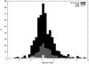 |
Fig. 1 Distribution of the 1.4 GHz to 2.4 GHz spectral indices found in the general source population, in the subsample containing AGN, and in our IFRS sample. |
3.1.3. Changes in the spectral index
The 4.8 GHz and 8.6 GHz observations have higher resolution than the 1.4 GHz and 2.4 GHz observations, and are less sensitive to extended emission. The spectral index between 4.8 GHz and 2.4 GHz is therefore not physically meaningful, because the data at the higher frequency are sensitive to more compact structures than the 1.4 GHz and 2.4 GHz observations. However, within each pair of bands (1.4 GHz/2.4 GHz or 4.8 GHz/8.6 GHz) the uv coverage has been matched and so the spectral indices are physically relevant to the size scale being studied.
We compared the low-frequency (1.4 GHz/2.4 GHz) and high-frequency (4.8 GHz/8.4 GHz) spectral indices of 10 targets, 7 of which have measured flux densities at 1.4 GHz, 2.4 GHz, 4.8 GHz, and 8.6 GHz, and 3 of which have upper limits at 8.6 GHz. In these cases, we used 3 times the image rms as an upper limit on the flux density to compute the spectral index (the comparatively small span in frequency enlarges the error bars in these cases). We show in Fig. 2 these two spectral indices and indicate with a straight line where they would be equal. Clearly the spectra steepen towards higher frequencies.
We note that the median  of all IFRS is lower
than the median
of all IFRS is lower
than the median  of the 10 sources which
also have a measurement or limit for
of the 10 sources which
also have a measurement or limit for  . This is (i)
because of the selection effect that the very steep-spectrum sources tend to have
escaped detection at the higher frequencies; and (ii) because of the use of upper limits
at 8.6 GHz, meaning that the true spectral index in these three cases is lower than
specified by us.
. This is (i)
because of the selection effect that the very steep-spectrum sources tend to have
escaped detection at the higher frequencies; and (ii) because of the use of upper limits
at 8.6 GHz, meaning that the true spectral index in these three cases is lower than
specified by us.
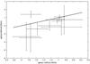 |
Fig. 2 The high-frequency spectral index, |
3.1.4. Discrepancy between low-frequency spectral index and higher-frequency lower limits
In some cases (CS538, ES318, ES419, ES749, ES798, and ES973) the spectral index derived from lower-frequency observations predicts 4.8 GHz or 8.6 GHz flux densities which are incompatible with the measurements at these frequencies. However, in some other cases such as CS703, ES427, or ES509 the detections at the highest frequencies align very well with the lower frequencies, and tightly follow power-laws. We consider this as evidence that the calibration is not systematically wrong since the same methods were used in all cases. Instead we consider two effects as potential causes of this discrepancy.
-
(i)
Sources are resolved out. The 843 MHz, 1.4 GHz and 2.4 GHz data have excellent uv coverage at spacings below 5 kλ (which corresponds to an angular scale of 41.25 arcsec), and even have good coverage at spacings shorter than 1 kλ (3.43 arcmin). On the other hand, in our matched-resolution images at 4.8 GHz and 8.6 GHz the shortest baseline used was 7 kλ (29.5 arcsec – note that one goal of these observations was to image the targets with high resolution, hence long baselines were selected). This means that even tapered images cannot reveal large-scale structure since this information simply is not in the data. However, when the angular resolution is converted to a linear scale one finds that to resolve objects out in these cases they must be relatively large. At redshifts of 0.1, 0.5 and 1, a resolution of 29.5 arcsec corresponds to 54 kpc, 179 kpc, and 237 kpc, respectively (using H0 = 71.0, ΩM = 0.27, Ωvac = 0.73). Only jets and lobes of radio galaxies are so large, and this would have been noticed in the 1.4 GHz images, as is the case in ES011. However, the majority of the sources suffering from high-frequency drop-outs are not visibly resolved, and given these size constraints we conclude that resolution is not the dominant effect. Furthermore, resolution can only explain spectra where both the 4.8 GHz and 8.6 GHz sensitivity limits are lower than what would be expected from the lower-frequency data.
-
(ii)
In cases where only the 8.6 GHz limit is below the extrapolation (as in, e.g., ES798 and ES973) resolution effects cannot account for the observed discrepancy because we carefully selected baselines such as to obtain matched-resolution images. In these cases, the spectral steepening must be related to the distribution of the particle energies in the source. In general, a population of particles with a power-law distribution of energies (with index q) in a uniform magnetic field will result in synchrotron emission with a constant radio spectral index with α = (1 − q)/2. Unless fresh particles are continuously injected into the source, the particles with higher energies will lose their energy faster than lower-energy particles, and the spectrum will steepen. Hence steeper spectra at higher frequencies could indicate that the AGN has recently been inactive.
 and
, the
median spectral index changes from −1.14 to a median of −1.71. This difference of
Δα = 0.57 is comparable to the change in α reported
by Readhead et al. (1996) in the prototypical CSS
source COINS J2355+4950, which was found to be 0.6. Whilst this similarity is prone to
coincidence and small-number statistics we note that Middelberg et al. (2008a) already pointed out the similarities between CSS
sources and a VLBI-detected IFRS.
and
, the
median spectral index changes from −1.14 to a median of −1.71. This difference of
Δα = 0.57 is comparable to the change in α reported
by Readhead et al. (1996) in the prototypical CSS
source COINS J2355+4950, which was found to be 0.6. Whilst this similarity is prone to
coincidence and small-number statistics we note that Middelberg et al. (2008a) already pointed out the similarities between CSS
sources and a VLBI-detected IFRS.
3.1.5. Polarisation
We also searched for polarised emission in our targets. We are in the process of making a careful analysis of the polarisation levels in the ATLAS radio data, accounting correctly for the positivity bias in images of polarised intensity (Hales et al. 2010, in prep.). A preliminary result is that three sources in our sample are significantly polarised at 1.4 GHz, whereas upper limits were obtained for the remaining 14 sources. The polarised sources are ES509 (P = 2.70 ± 0.03 mJy), ES973 (P = 0.83 ± 0.06 mJy), and CS703 (P = 1.90 ± 0.05 mJy). All other sources are unpolarised at the various levels indicated in Table 1. The limits are given at >99% credibility (Bayesian confidence) that sources are unpolarised (Vaillancourt 2006).
3.1.6. Radio-24 μm flux density ratio
It is well-established that there is a tight correlation, extending over five orders of magnitude, between the radio and far-infrared (FIR) luminosity, or flux density, of star-forming galaxies (van der Kruit 1973; Condon et al. 1982; Dickey & Salpeter 1984; de Jong et al. 1985). It is attributed to massive star formation, which generates far-infrared emission by heating dust, and generates radio emission by accelerating cosmic rays that then generate radio synchrotron radiation. However, since far-infrared telescopes are relatively insensitive, the 24 μm flux density is often used as an imperfect proxy for the FIR flux density (Appleton et al. 2004). While the 24 μm flux density is subject to other emission mechanisms than warm dust, especially at high redshift, it remains clear (Seymour et al. 2008) that a high value of the radio-24 μm flux density ratio indicates the presence of an AGN.
We note that since all our IFRS targets have S1.4 GHz > 1 mJy and are undetected not only at 3.6 μm but also at 24 μm, with a 5σ limit of S24 μm = 252 μJy, their q24 = log (S24 μm/S20 cm) values are lower than log(252 μJy/1000 μJy) = −0.60. The radio-IR relation for star forming galaxies has been determined to yield q24 = 0.84 ± 0.28 (Appleton et al. 2004), so all IFRS have a more than tenfold radio excess over this relation. The common interpretation of this is that synchrotron radiation is being produced without IR emission, which then is regarded as evidence for non-thermal emission from an AGN. Therefore, all IFRS can be classified as AGN based on q24 alone.
3.2. IFRS and high-redshift radio galaxies
There are two main tools for finding radio galaxies at high redshifts. The so-called z−α relation is derived from the observation that steep-spectrum radio galaxies tend to have higher redshifts (De Breuck et al. 2002; Klamer et al. 2006). Many high-redshift radio galaxies (HzRG) have been found exploiting this relation. The other tool is the K − z relation (Lilly & Longair 1984) which states that the logarithm of an object’s redshift is proportional to the near-IR K-band magnitude at 2.2 μm. A combination of these two criteria can be used as an efficient filter for HzRG.
3.2.1. The ratio of the 1.4 GHz and 3.6 μm flux densities
We used the widely-used Spitzer 3.6 μm band as a proxy for K-band observations. It has been argued previously (Middelberg et al. 2008b; Garn & Alexander 2008; Huynh et al. 2010; Norris et al. 2010) that the SEDs of IFRS are compatible with those of high-redshift AGN. We therefore compiled S20/S3.6 values for the sample of 70 high-redshift radio galaxies (HzRG) by Seymour et al. (2007), to compare them to the general radio population and the IFRS. Seymour et al. (2007) selected from the literature radio galaxies above a redshift of one with a 3 GHz luminosity of more than 1026 W/Hz, and supplemented their sample with new or archival Spitzer data. IFRS are selected based on the ratio of the radio and IR flux densities. Sources in the ATLAS radio catalogues typically have flux densities exceeding 100 μJy (5σ), whereas the co-spatial 3.6 μm observations have 1σ sensitivities of around 1 μJy. Therefore a detected radio source with no catalogued or visibly identifiable counterpart (i.e., S3.6 μm < 3σ = 3 μJy) typically has S20/S3.6 > 30. However, the median S20/S3.6 ratio of the IFRS in our sample is 2330, some two orders of magnitude larger than this minimum. Hence, while sources with S20/S3.6 > ≈50 could be starbursts or AGN-driven, at S20/S3.6 exceeding a few hundred are likely to be similar to the HzRG.
The median S20/S3.6 ratio of all sources in the ATLAS/ELAIS field (with detections in both the radio and IR bands) is 6.12, but the distribution extends over five orders of magnitude. With ratios between approximately 500 and 10 000, the IFRS clearly are at and beyond the high tail of the distribution of the general source population.
The median S20/S3.6 of the HzRG by Seymour et al. (2007) is 6550, significantly larger than in the general source population, and closer to the IFRS median. However, HzRG are much brighter – they present high luminosities and have been gathered from surveys covering much larger areas. In contrast, IFRS are fainter (by a factor of around 50 if they are assumed to be at the same redshifts as HzRG) and have a surface density of around 10 deg-2, whereas that of HzRG is 0.001 deg-2 – approximately four orders of magnitude smaller. A histogram of S20/S3.6 of the general radio source population, the HzRG and the IFRS is shown in Fig. 3.
We stress that since for IFRS S20/S3.6 has been calculated using upper limits on the 3.6 μm flux density, the true ratio is expected to be larger. Given the stacking experiments by Norris et al. (2010), who find that the median flux density of IFRS 3.6 μm counterparts is less than 0.2 μJy, we point out that the S20/S3.6 ratios of IFRS could be as much as a factor of 5 higher than estimated here. This would shift the IFRS in Fig. 3 to the right by log(5) = 0.7 (illustrated in the lower panel of Fig. 3). The median S20/S3.6 of the IFRS then increases to 11650, almost two times the HzRG median.
Norris et al. (2010) also show that IFRS are consistent with radio-loud AGN at redshifts greater than 3. They used observations from the Spitzer Warm Mission (5σ limits of 1 μJy, 5 times deeper than the Spitzer SWIRE data) and the published ATLAS radio catalogues. All of their IFRS remain undetected even with these new observations. They argue that, since the S20/S3.6 ratios are of the same order of magnitude as the HzRG by Seymour et al. (2007), and since the 3.6 μm flux densities of HzRG drop below the Spitzer detection limit when at redshifts larger than 3, IFRS are likely to be at similarly high redshifts.
Huynh et al. (2010) analysed four IFRS in the GOODS/CDFS, which are located in a region for which very deep Spitzer data had recently become available. They find counterparts for only two of the IFRS, CS446, and CS506, yielding S20/S3.6 ratios of 51.2 and 30.9, respectively. The two IFRS still undetected with the new Spitzer data, CS283 and CS415, have S20/S3.6 ratios of >137 and >2520, respectively. CS415 has a radio spectral index of −1.1 but was not included in our sample because it was deemed too faint for successful 4.8 GHz and 8.6 GHz observations.
 |
Fig. 3 Top panel: the distribution of S20/S3.6 in the general source population, in the sample of HzRG by Seymour et al. (2007), and in our IFRS sample. The IFRS clearly occupy a different regime than the general population, and tend to overlap more with the HzRG. Bottom panel: the histogram of the IFRS S20/S3.6 ratios as in the upper panel, shifted to the right by log(5) = 0.7. This takes into account that Norris et al. (2010) found no IR counterparts for IFRS in a stacking analysis with a 5 times higher sensitivity. On average the IFRS then have a S20/S3.6 which is about two times higher than that of the HzRG. |
From the histogram of S20/S3.6 it becomes clear that there is more overlap between IFRS and HzRG than between IFRS and the general radio source population. IFRS appear to have steep radio spectra and very faint IR flux densities, both of which indicate that they are high-redshift AGN.
One could argue that IFRS-like sources exist in the data which are not classified as such because they are above the SWIRE 3.6 μm detection limit, but have similar S20/S3.6 ratios. There are 16 non-IFRS in the ATLAS/ELAIS catalogue with S20/S3.6 exceeding 500, the minimum found among the IFRS. All these sources were classified as AGN, based on either radio morphology or because of their clear (10-fold) excess over the radio-infrared relation (some do not have a detected 24 μm counterpart, so the 5σ detection limit of 252 μJy was assumed). There are 66 more sources with S20/S3.6 between 100 and 500, all of which were classified as AGN based on q24 = log (S24 μm/S20 cm) (Appleton et al. 2004, using a 252 μJy limit in case of non-detections). Hence we argue that an excess of radio over 3.6 μm, like q24, can be regarded as an indicator of non-thermal emission from AGN, and that this finding supports the hypothesis that IFRS host AGN. Out of the 82 sources in the ATLAS/ELAIS catalogue with measured S20/S3.6 in excess of 100, 6 have a spectroscopic redshift. The median of these redshifts is 0.38, and only a single object has a redshift larger than 1, with z = 1.82. We conclude that objects with measured S20/S3.6 in the same range as IFRS could indeed be similar objects at lower redshifts.
We also computed S20/S3.6 for the submm-detected sources of the SCUBA-SHADES survey (Clements et al. 2008; Ivison et al. 2007). We find that these sources in general have rather low S20/S3.6 values, of the order of a few, with only three exceeding 10. This result is consistent with them being starburst galaxies.
3.2.2. The spectral indices of IFRS and HzRG
We show in Fig. 4 the distribution of the spectral
indices of IFRS and the spectral indices of the HzRG by Seymour et al. (2007). The median of the IFRS sample is
 , whereas the median of
the HzRG sample is −1.02. Given the z − α relation
this indicates that IFRS are located at even higher redshifts than the HzRG. A K-S-test
shows with p = 0.011 that the two distributions are unlikely to be
drawn from the same parent distribution.
, whereas the median of
the HzRG sample is −1.02. Given the z − α relation
this indicates that IFRS are located at even higher redshifts than the HzRG. A K-S-test
shows with p = 0.011 that the two distributions are unlikely to be
drawn from the same parent distribution.
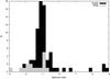 |
Fig. 4 The distribution of the spectral indices of IFRS and HzRG. The median of the IFRS
sample is |
3.2.3. Simulated surface densities of radio emitters
The extragalactic part of the SKA simulated skies, S3-SEX (Wilman et al. 2010), is a simulation of radio continuum sources in an area of 20 × 20 deg2 out to redshift z = 20. It represents today’s knowledge about the radio sky and is used as reference when predictions are needed for the findings with new telescopes such as Lofar and the SKA pathfinders.
We queried S3-SEX for star-forming galaxies, quasars, and FR I and FR II radio galaxies with a 1.4 GHz flux density exceeding 1 mJy. In a first query, we searched for sources at z > 2 and in a second query for sources with z > 4. Our findings are listed in Table 2.
We find that the surface densities of star-forming galaxies and radio quasars is too low by orders of magnitude to account for the IFRS phenomenon. FR I/II sources, however, have much higher surface densities, even higher than the number of IFRS in our sample. Therefore they could account for at least a fraction of the IFRS. However, the observations presented here and by Middelberg et al. (2008b) indicate that in general such objects are too large.
Surface densities of various types of radio sources taken from the extragalactic part of the SKA simulated sky.
3.3. Notes on individual sources and their classification
Here we describe the individual targets.
-
ES 509 is a strong, compact radio source at 1.4 GHz and is detected at all other frequencies. Its spectrum is a well-defined power-law with an index of −1.02, and its S20/S3.6 ratio is 9240, clearly in the realm of the HzRG sample by Seymour et al. (2007). It is significantly polarised at 1.4 GHz (12%) and also at higher frequencies. We conclude from this evidence that this is an AGN. However, this source was not detected by Middelberg et al. (2008b) in VLBI observations, who determined that its compact flux density was lower than 0.27 mJy at 1.4 GHz.
-
ES 427 is similar to ES 509 in that it is a strong, compact radio source at 1.4 GHz with a spectral index of −1.08, and has a S20/S3.6 ratio of 9070. However, there are two significant differences to ES 509: ES 427 is unpolarised in all our radio images (<1%), but was detected and imaged by Middelberg et al. (2008b) using VLBI, who suggested that its properties are consistent with it being a CSS. We therefore conclude that this is an AGN.
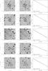
Fig. 5 Each row shows a grey-scale image of the Spitzer 3.6 μm observations, superimposed with grey contours indicating the 1.4 GHz observations and black contours showing the 4.8 GHz (left panel) and 8.6 GHz (middle panel) observations. The IFRS are always the sources at the image centres. Contours start at 3σ and increase by factors of 2. The 1.4 GHz restoring beam and the 4.8 GHz/8.6 GHz restoring beams, which are the same size, are indicated with ellipses in the lower left corners of the images. The right panel shows the flux density measurements available for a source and 3σ upper limits where no detection was made (indicated with arrows). The solid line indicates the best available spectral index, and dashed lines indicate a power-law with an index 1σ larger and 1σ smaller than determined by the data. We note that all sources have a signal-to-noise ratio of more than 9 in the 1.4 GHz observations, so there is no doubt that they are real sources and not spurious.
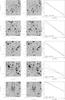
Fig. 5 continued.
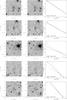
Fig. 5 continued.
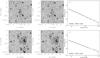
Fig. 5 continued.
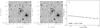
Fig. 6 The high-frequency images of CS487 clearly show an association of the radio emission with the infrared source SWIRE3_J033300.99-284716.6, and hence is no longer classified as IFRS.
-
ES 973 is an extended radio source at 1.4 GHz which has been classified as AGN based on this finding alone, but its S20/S3.6 ratio of 4710 supports this. Its spectrum is steep with an index of −1.15, but it is not detected at 8.6 GHz, where, according to an extrapolation from the lower frequencies, a 13.3σ detection would have been expected. It is polarised at 1.4 GHz (7%) and unpolarised at 4.8 GHz. Therefore, based on morphology and polarisation, this is an AGN.
-
ES 798 is a somewhat extended radio source at 1.4 GHz, and the detection at 4.8 GHz pinpoints a position which suggests that the nearby IR source is not associated, as had already been suggested by Middelberg et al. (2008a). Its S20/S3.6 ratio is 4760 which is high, and its spectral index of −0.81 is not well-defined. The non-detection at 8.6 GHz is odd since a 14.6σ detection would have been expected. It is unpolarised at 1.4 GHz (<5%), but still we deem the evidence based on radio morphology and S20/S3.6 sufficient to classify this source as an AGN.
-
ES 749 is a somewhat extended radio source at 1.4 GHz with a high S20/S3.6 of 4170. Its extended morphology suggests that it is AGN-driven, and this is confirmed by its rather steep spectrum with index −1.08. Its 8.6 GHz flux density is lower than expected from lower-frequency extrapolation, and it is unpolarised (<7%). We classify this source as an AGN.
-
ES 775 is another extended (at 1.4 GHz) radio source with a S20/S3.6 ratio of 1360 and a steep spectrum with index −1.35. A faint bridge of emission extends towards the nearby source ES 780, and the nature of this bridge is unclear. ES775 is not detected at 8.6 GHz due to sensitivity limits, and it is unpolarised (<6%). Middelberg et al. (2008b) found that in VLBI observations the compact emission from this source was less than 0.26 mJy at 1.6 GHz, however, the arcsec-scale morphology and steep spectrum lead us to conclude that this source is AGN-driven.
-
ES 011 is a significantly extended source at 1.4 GHz with a high S20/S3.6 ratio of 3870 and a steep, albeit somewhat ill-defined, radio spectrum with index −1.44. The 1.4 GHz emission appears too high, part of which we ascribe to confusion with nearby sources (the flux density being measured from a low-resolution image). If confusion is indeed an issue, the flux density at the lower three frequencies could be over-estimated, and therefore the non-detections at 4.8 GHz and 8.6 GHz would not be significant. ES011 is unpolarised (<6%), and therefore we find no strong evidence that this source contains an AGN.
-
ES 419 is a compact 1.4 GHz radio source with a moderately high S20/S3.6 ratio of 1800. This source was deemed by Middelberg et al. (2008a) not to be associated with the nearby IR objects visible in Fig. 5. Its lower-frequency radio spectral index is a rather steep −1.35, and it has not been detected at the higher frequencies because of its faintness. It is unpolarised (<5%), and so the only clues to its classification are S20/S3.6 and α, and we tentatively identify this source as an AGN.
-
ES 318 is a slightly extended, faint 1.4 GHz radio source with an ill-defined spectral index of −0.78 and a moderate S20/S3.6 ratio of 820. It is unpolarised (<10%), but we do not have sufficient evidence to make a reasonable classification.
-
CS 703 is a very compact, strong radio source with a well-defined, rather steep spectrum with index −0.99 and a high S20/S3.6 ratio of 8980. The non-detection at 74 MHz can probably be attributed to synchrotron self-absorption. It is polarised at all frequencies (7% at 1.4 GHz), and since we do not see any evidence of it being resolved, we classify this source as an AGN.
-
CS 114 is a compact radio source at all frequencies with a steep spectrum (α = −1.34) and a high S20/S3.6 of 2560. It is known to be an AGN because of its VLBI-detected compact core (Norris et al. 2007) which contains 5 mJy and thus most of the total emission. It is unpolarised (<3%), but we suggest it is AGN-driven.
-
CS 194 is a compact radio source at all frequencies and does have a steep spectrum with index −1.12 and an S20/S3.6 ratio of 2330. Norris et al. (2007) do not detect this source in a VLBI observation and conclude that if it contains an AGN its compact emission must be less than 1 mJy. Hence its emission is compact enough to be unresolved at a few arcsec, but extended enough to be resolved out on the shortest LBA baseline with a resolution of 390 mas. It is one of the two sources which have a higher spectral index at the higher frequencies, and was not found to be polarised (<3% at 1.4 GHz) at any frequency. We do not have sufficient evidence to conclusively classify this source as an AGN.
-
CS 538 is a faint, slightly extended 1.4 GHz radio source, for which we only have two flux density measurements, yielding a spectral index of −0.88. Its S20/S3.6 ratio is 650, and the non-detections at 4.8 GHz and 8.6 GHz are due to its faintness. The 1.4 GHz emission is extended towards a nearby IR source, but unless higher-resolution imaging is provided an association remains unclear. It is unpolarised at 1.4 GHz (<10%). Hence it can not be classified reliably as an AGN.
-
CS 241 is another faint, unpolarised (<12%) 1.4 GHz radio source with a remarkably steep, but ill-defined, spectral index of −1.96 and an S20/S3.6 ratio of 540. Its classification remains unclear due to its faintness.
-
CS 415 is a radio source with a remarkably steep spectrum (α = −2.38), even though this is not well-defined. Its S20/S3.6 ratio is still high (880) compared to the general radio population, and it is unpolarised (<8% at 1.4 GHz). Its classification is unclear.
-
CS 164 is a 1.6 mJy radio source at 1.4 GHz with a well-defined spectral index of −0.92 and an S20/S3.6 ratio of 530, placing it at the lower end of the IFRS distribution. Like most sources it is unpolarised at 1.4 GHz (<13%), and we therefore do not have reliable evidence that this is an AGN.
-
CS 215 is a faint radio source with a “normal” spectral index of −0.76 and has at 520 the lowest S20/S3.6 ratio in our sample. At 2.4 GHz the source merges with other nearby radios sources and we were unable to measure its flux density there. The SED suggests that the 1.4 GHz data point is flattening the spectrum somewhat, but this is speculative. The source is unpolarised (<13% at 1.4 GHz), and our evidence therefore is not sufficient to classify this as an AGN.
4. Conclusions
We compiled radio observations of a sample of IFRS, and added dedicated high-frequency, high-resolution observations to investigate the nature of these objects. Using the IR detection limits we computed their ratio of 1.4 GHz to 3.6 μm flux density and compared them with the general radio source population and a sample of high-redshift radio galaxies. Our conclusions are as follows.
-
All IFRS can be classified as AGN based on their radio excess over the radio-IR relation. This is encapsulated in all of them having a value of q24 of less than −0.60.
-
The distribution of the IFRS spectral indices is significantly different from the distribution of the general radio source population, and also different from the AGN population. The spectra are steep, with a median of
, which is much steeper
than the spectral indices of a sample of HzRG by Seymour et al. (2007), who found a median of −1.02. Also there is a
prominent lack of spectral indices larger than −0.7. The very steep radio spectra
indicate a fundamental difference to the general radio source population. -
We find tentative evidence that radio spectra are steepening towards higher frequencies, indicating synchrotron losses. The spectra display curvature seen in CSS/GPS sources rather than the power-law more typical of classical AGN.
-
The ratio of 1.4 GHz flux density to 3.6 μm flux density, S20/S3.6, is biased to much higher values than that of the general radio source population, and has significant overlap with the HzRG distribution of the Seymour et al. (2007) sample. Whilst the HzRG are very rare sources selected from all-sky surveys with very high luminosities, IFRS could be a less luminous, but much more abundant version of AGN-driven sources at very high redshifts.
-
Out of the 18 sources discussed here, one (CS487) has been de-classified as IFRS because its radio emission showed a solid association with a nearby IR source. Out of the 17 remaining sources, 10 have been classified as AGN based on either their S20/S3.6 ratio (9), polarisation properties (4), radio spectral index (4), a VLBI detection (2) and radio morphology (3).
-
7 sources have insufficient data to yield a positive AGN classification (except for their value of q24), mostly because our radio data were not sufficiently sensitive.
References
- Appleton, P. N., Fadda, D. T., Marleau, F. R., et al. 2004, ApJS, 154, 147 [NASA ADS] [CrossRef] [Google Scholar]
- Bock, D. C.-J., Large, M. I., & Sadler, E. M. 1999, AJ, 117, 1578 [NASA ADS] [CrossRef] [Google Scholar]
- Carilli, C. L., Owen, F. N., & Harris, D. E. 1994, AJ, 107, 480 [NASA ADS] [CrossRef] [Google Scholar]
- Clements, D. L., Vaccari, M., Babbedge, T., et al. 2008, MNRAS, 387, 247 [NASA ADS] [CrossRef] [Google Scholar]
- Cohen, A. S., Lane, W. M., Cotton, W. D., et al. 2007, AJ, 134, 1245 [NASA ADS] [CrossRef] [Google Scholar]
- Condon, J. J., Condon, M. A., Gisler, G., & Puschell, J. J. 1982, ApJ, 252, 102 [NASA ADS] [CrossRef] [Google Scholar]
- De Breuck, C., Tang, Y., de Bruyn, A. G., Röttgering, H., & van Breugel, W. 2002, A&A, 394, 59 [NASA ADS] [CrossRef] [EDP Sciences] [Google Scholar]
- de Jong, T., Klein, U., Wielebinski, R., & Wunderlich, E. 1985, A&A, 147, L6 [NASA ADS] [Google Scholar]
- Dickey, J. M., & Salpeter, E. E. 1984, ApJ, 284, 461 [NASA ADS] [CrossRef] [Google Scholar]
- Garn, T., & Alexander, P. 2008, MNRAS, 391, 1000 [NASA ADS] [CrossRef] [Google Scholar]
- Huynh, M. T., Norris, R. P., Siana, B., & Middelberg, E. 2010, ApJ, 710, 698 [NASA ADS] [CrossRef] [Google Scholar]
- Ivison, R. J., Greve, T. R., Dunlop, J. S., et al. 2007, MNRAS, 380, 199 [Google Scholar]
- Jarvis, M. J., Rawlings, S., Eales, S., et al. 2001, MNRAS, 326, 1585 [NASA ADS] [CrossRef] [Google Scholar]
- Klamer, I. J., Ekers, R. D., Bryant, J. J., et al. 2006, MNRAS, 371, 852 [NASA ADS] [CrossRef] [Google Scholar]
- Lacy, M., Afonso, J., Appleton, P. N., et al. 2010, ApJ, submitted [Google Scholar]
- Ledlow, M. J., & Owen, F. N. 1996, AJ, 112, 9 [NASA ADS] [CrossRef] [Google Scholar]
- Lilly, S. J., & Longair, M. S. 1984, MNRAS, 211, 833 [NASA ADS] [CrossRef] [Google Scholar]
- Lonsdale, C. J., Smith, H. E., Rowan-Robinson, M., et al. 2003, PASP, 115, 897 [NASA ADS] [CrossRef] [Google Scholar]
- Manchester, R. N., Hobbs, G. B., Teoh, A., & Hobbs, M. 2005, AJ, 129, 1993 [NASA ADS] [CrossRef] [Google Scholar]
- Middelberg, E., Norris, R. P., Cornwell, T. J., et al. 2008a, AJ, 135, 1276 [NASA ADS] [CrossRef] [Google Scholar]
- Middelberg, E., Norris, R. P., Tingay, S., et al. 2008b, A&A, 491, 435 [NASA ADS] [CrossRef] [EDP Sciences] [Google Scholar]
- Moretti, A., Campana, S., Lazzati, D., & Tagliaferri, G. 2003, ApJ, 588, 696 [NASA ADS] [CrossRef] [Google Scholar]
- Murgia, M. 2003, Publications of the Astronomical Society of Australia, 20, 19 [Google Scholar]
- Norris, R. P., Afonso, J., Appleton, P. N., et al. 2006, AJ, 132, 2409 [NASA ADS] [CrossRef] [Google Scholar]
- Norris, R. P., Afonso, J., Cava, A., et al. 2010, ApJ, accepted [Google Scholar]
- Norris, R. P., Tingay, S. J., Phillips, C., et al. 2007, MNRAS [Google Scholar]
- Pentericci, L., Van Reeven, W., Carilli, C. L., Röttgering, H. J. A., & Miley, G. K. 2000, A&AS, 145, 121 [Google Scholar]
- Readhead, A. C. S., Taylor, G. B., Xu, W., et al. 1996, ApJ, 460, 612 [NASA ADS] [CrossRef] [Google Scholar]
- Sault, R. J., Teuben, P. J., & Wright, M. C. H. 1995, in Astronomical Data Analysis Software and Systems IV, ASP Conf. Ser., 77, 433 [Google Scholar]
- Seymour, N., Dwelly, T., Moss, D., et al. 2008, MNRAS, 386, 1695 [NASA ADS] [CrossRef] [Google Scholar]
- Seymour, N., Stern, D., De Breuck, C., et al. 2007, ApJS, 171, 353 [NASA ADS] [CrossRef] [Google Scholar]
- Vaillancourt, J. E. 2006, PASP, 118, 1340 [Google Scholar]
- van der Kruit, P. C. 1973, A&A, 29, 263 [NASA ADS] [Google Scholar]
- Wilman, R. J., Jarvis, M. J., Mauch, T., Rawlings, S., & Hickey, S. 2010, MNRAS, 405, 447 [NASA ADS] [Google Scholar]
All Tables
Surface densities of various types of radio sources taken from the extragalactic part of the SKA simulated sky.
All Figures
|
Fig. 1 Distribution of the 1.4 GHz to 2.4 GHz spectral indices found in the general source population, in the subsample containing AGN, and in our IFRS sample. |
| In the text | |
|
Fig. 2 The high-frequency spectral index, |
| In the text | |
|
Fig. 3 Top panel: the distribution of S20/S3.6 in the general source population, in the sample of HzRG by Seymour et al. (2007), and in our IFRS sample. The IFRS clearly occupy a different regime than the general population, and tend to overlap more with the HzRG. Bottom panel: the histogram of the IFRS S20/S3.6 ratios as in the upper panel, shifted to the right by log(5) = 0.7. This takes into account that Norris et al. (2010) found no IR counterparts for IFRS in a stacking analysis with a 5 times higher sensitivity. On average the IFRS then have a S20/S3.6 which is about two times higher than that of the HzRG. |
| In the text | |
|
Fig. 4 The distribution of the spectral indices of IFRS and HzRG. The median of the IFRS
sample is |
| In the text | |
|
Fig. 5 Each row shows a grey-scale image of the Spitzer 3.6 μm observations, superimposed with grey contours indicating the 1.4 GHz observations and black contours showing the 4.8 GHz (left panel) and 8.6 GHz (middle panel) observations. The IFRS are always the sources at the image centres. Contours start at 3σ and increase by factors of 2. The 1.4 GHz restoring beam and the 4.8 GHz/8.6 GHz restoring beams, which are the same size, are indicated with ellipses in the lower left corners of the images. The right panel shows the flux density measurements available for a source and 3σ upper limits where no detection was made (indicated with arrows). The solid line indicates the best available spectral index, and dashed lines indicate a power-law with an index 1σ larger and 1σ smaller than determined by the data. We note that all sources have a signal-to-noise ratio of more than 9 in the 1.4 GHz observations, so there is no doubt that they are real sources and not spurious. |
| In the text | |
|
Fig. 5 continued. |
| In the text | |
|
Fig. 5 continued. |
| In the text | |
|
Fig. 5 continued. |
| In the text | |
|
Fig. 6 The high-frequency images of CS487 clearly show an association of the radio emission with the infrared source SWIRE3_J033300.99-284716.6, and hence is no longer classified as IFRS. |
| In the text | |
Current usage metrics show cumulative count of Article Views (full-text article views including HTML views, PDF and ePub downloads, according to the available data) and Abstracts Views on Vision4Press platform.
Data correspond to usage on the plateform after 2015. The current usage metrics is available 48-96 hours after online publication and is updated daily on week days.
Initial download of the metrics may take a while.