© ESO, 2011

1. Introduction

The Planck satellite mission, currently in flight, will provide measurements of the CMB anisotropies both in temperature and polarization over the full sky at unprecedented accuracy. Planck, which observes the sky over a wide range of frequency bands from 30 to 857 GHz, has a combined sensitivity of $\frac{\mathrm{\Delta }\mathit{T}}{{\mathit{T}}_{\mathrm{CMB}}}\mathrm{~}\mathrm{2}\mathrm{\times }{\mathrm{10}}^{-6}$ and an angular resolution from 33 to 5 arcmin (Consortia 2004). Of particular cosmological interest is the possibility of measuring the so-called polarization B modes, the existence of which implies that tensor fluctuations from primordial gravitational waves are generated during inflation. Planck should be able to measure the tensor-to-scalar ratio, r, down to 0.1 (Betoule et al. 2009; Efstathiou et al. 2009) in the case of a nominal mission (2 full-sky surveys) and to 0.05 with an extended mission of 4 full-sky surveys (Efstathiou & Gratton 2009). The value of r sets the energy scale of inflation (Peiris et al. 2003) and then provides constraints on inflationary models (Baumann 2009).

To achieve this high level of sensitivity, it is necessary to accurately estimate the temperature and polarization foregrounds that arise both from diffuse Galactic emission components and from point-like and compact sources of Galactic and extragalactic origins. Indeed, in the Planck frequency bands these foreground components may dominate the polarized CMB signal and therefore must be either masked or subtracted prior to any CMB analysis. For this purpose, the Planck collaboration plans to use component separation techniques (see Leach et al. 2008, for a summary) in addition to the traditional masking of highly contaminated sky regions including identified point-like and compact sources. As these component separation techniques will be mainly based on Planck data alone, one of the main issues will be to estimate the residual foreground contamination on the final CMB temperature and polarization maps. These residuals will translate into systematic biases and larger error bars on the estimation of the temperature and polarization power spectra of the CMB fluctuations (see Betoule et al. 2009, for a recent study). Thus, they will affect the precision to which cosmological information can be retrieved from the Planck data.

The main polarized foreground contributions will come from the diffuse Galactic synchrotron and thermal dust emission. Using Wmap (Wilkinson Microwave Anisotropy Probe) observations, Page et al. (2007) have shown that the emission from relativistic electrons is highly polarized, up to 70%, between 23 and 94 GHz. Furthermore, Benoît et al. (2004); Ponthieu et al. (2005) have observed significantly polarized thermal dust emission, up to a level of 15% at the 353 GHz Archeops channel. By contrast the diffuse free-free emission is not intrinsically polarized and the anomalous dust-correlated microwave emission has been measured to be weakly polarized, ${\mathrm{3}}_{-1.9}^{\mathrm{+}\mathrm{1.3}}$% (Battistelli et al. 2006). Finally, at the Planck frequency bands the polarized contributions from compact and point sources are expected to be weak for both radio (Nolta 2009) and dust (Désert et al. 2008) sources. The spatial and frequency distribution of both Galactic synchrotron and thermal dust polarized emissions at the Planck frequencies are not well known and the only available informations come from microwave and submillimetre observations. For synchrotron, Faraday rotation (Burn 1966) makes it very difficult to extrapolate the polarized observed radio emissions (Wolleben et al. 2006; Wolleben 2007; Carretti 2009) to the microwave domain. For thermal dust, polarized observations are not currently available in the infrared and the current optical data (Heiles 2000) are too sparses (Page et al. 2007) for a reliable extrapolation to lower frequencies.

The diffuse Galactic synchrotron emission is produced by relativistic electrons spiraling around the Galactic magnetic field lines with the direction of polarized emission orthogonal both to the line-of-sight and to the field lines (Rybicki & Lightman 1979). Based on these statements, Page et al. (2007) proposed to model the polarized synchrotron Galactic emission observed by the Wmap satellite using a 3D model of the Galaxy including the distribution of relativistic electrons and the Galactic magnetic field structure. Although this model allowed them to explain the observed polarization angle at the 23 GHz band where the synchrotron emission dominates, it was not used for the CMB analysis. Instead, the 23 GHz data were adopted as a template for polarized synchrotron emission and extrapolated to higher frequencies. Independently, Han et al. (2004, 2006) used a 3D model of the free electrons in the Galaxy (Cordes & Lazio 2002) and of the Galactic magnetic field that included regular and turbulent components to explain the observed rotation measures towards known pulsars. Based on previous work, Sun et al. (2008) performed a combined analysis of the polarized Wmap data and of the rotation measurements of pulsars using the publicly available Hammurabi code (Waelkens et al. 2009) for computing the integrated emission along the line-of-sight. This work has been extended by Jaffe et al. (2010) for the study of the Galactic plane using an MCMC algorithm to explore the parameter space of the models, and by Jansson et al. (2009) for the full sky using a likelihood analysis for parameters estimation.

Thermal dust emission arised from dust grains in the Interstellar Medium (ISM) which are heated by stellar radiation (Désert et al. 1998). They are considered to be oblate in shape and to align their longitudinal axis perpendicularly to the magnetic field lines (Davis & Greenstein 1951). When aligned they rotate with their angular moment parallel to the magnetic field lines. Since the thermal dust emission is more efficient along the long axis, linear polarization is generated orthogonal to the magnetic field lines and to the line-of-sight. The polarization fraction of the emission depends on the size distribution of the grains and is about a few percent at millimeter wavelengths (Hildebrand et al. 1999; Vaillancourt 2002). Ponthieu et al. (2005) concluded that the polarized emission observed in the 353 GHz Archeops data was associated with the thermal dust emission and proposed a simple magnetic field pattern to explain the measured polarization on the Galactic plane. Page et al. (2007) suggested that part of the observed polarized emission of the 94 GHz Wmap data was also due to thermal dust. They modeled it using the observed polarization of stellar light (Heiles 2000) which has a direction perpendicular to that of thermal dust.

With the prospect of data from the Planck satellite mission in mind, we present here consistent physical models of the synchrotron and thermal dust emissions based on the 3D distribution of relativistic electrons and dust grains in the Galaxy, and on a 3D pattern of the Galactic magnetic field. The paper is structured as follows: Sect. 2 describes the 408 MHz all-sky continuum survey (Haslam et al. 1982), the five-year Wmap data set (Page et al. 2007) and the Archeops data (Ponthieu et al. 2005) used in the analysis. In Sect. 3 we describe in detail models for the polarized emissions, which are statistically compared to the data in Sect. 4. In Sect. 5 we discuss the impact of polarized foregrounds on the measurement of the polarized CMB emission with the Planck satellite, before presenting our conclusions in Sect. 6.

2. Observational data

2.1. Diffuse Galactic synchrotron emission

The synchrotron mechanism emission is an important contributor to the diffuse sky emissions at both radio and microwave observation frequencies. Although its SED is not accurately known, it is considered to be well represented by a power law in antenna temperature ${\mathit{T}}_{\mathit{\nu }}\mathrm{\propto }{\mathit{\nu }}_{\mathrm{s}}^{\mathit{\beta }}$ with the synchrotron spectral index ranging from  − 2.7 to  − 3.3 (Kogut et al. 2007; Gold et al. 2009). Radio frequency information such as the Leiden 408 MHz and 1.4 GHz surveys (Brouw & Spoelstra 1976; Wolleben et al. 2006), the Parkes survey at 2.4 GHz (Duncan et al. 1999), and the MGLS survey (Medium Galactic Latitude Survey) at 1.4 GHz (Uyaniker et al. 1999) are generally used to provide insight the Galactic diffuse synchrotron emission in polarized intensity. However, Faraday rotation introduces complications into the interpretation of such data since strong depolarization is expected for frequencies lower than 10 GHz (Burn 1966; Sun et al. 2008; Jaffe et al. 2010; Jansson et al. 2009; La Porta et al. 2008, 2006). Consequently, the best polarized Galactic diffuse synchrotron tracers are at high frequency such as the Wmap survey at 23 GHz (Page et al. 2007).

2.1.1. 408 MHz all-sky continuum survey

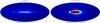Fig. 1 Intensity maps at 408 MHz in KRJ units for the Haslam data (left) and built with the model of synchrotron emission with an MLS magnetic field for the best fit model parameters (right).

In the following we use the 408 MHz all sky continuum survey (Haslam et al. 1982) as a tracer of the Galactic synchrotron emission in temperature. We use the HEALPix (Gòrski et al. 2005) format map available on the LAMBDA website¹. The calibration scale of this survey is claimed to be accurate to better than 10% and the zero level has an uncertainty of  ± 3 K as explained in Haslam et al. (1982). To subtract the free-free emission at 408 MHz we use the five-year public Wmap free-free foreground map at 23 GHz generated from the maximum entropy method (MEM) described in Hinshaw et al. (2007). We have found that the free-free correction has no impact on the final results presented in this paper. We start from the full sky HEALPix maps at N_side = 512 (pixel size of 6.9 arcmin) and downgrade them to N_side = 32 (pixel size of 27.5 arcmin). We then subtract from the Haslam data the free-free component extrapolated from the K-band assuming a power-law dependence of ν^-2.1 as in Dickinson et al. (2003). The left panel of Fig. 1 shows the free-free corrected 408 MHz all-sky survey where we clearly observe the Galactic plane and the north polar spur at high Galactic latitude.

2.1.2. Five-year WMAP polarized data at 23 GHz

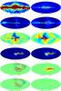Fig. 2 Form top to bottom: maps in intensity, I, and polarization Q and U at 23 GHz for the WMAP 5-year data (left) and the model of synchrotron emission with MLS magnetic field for the best fit model parameters (right) and at 353 GHz for the Archeops data (left) and the model of thermal dust emission with MLS magnetic field for the best fit model parameters (right). The 353 GHz maps are rotated by 180° for better visualization. All the maps are in KRJ units.

To trace the polarized synchrotron emission we used the all sky five-year WmapQ and U maps at 23 GHz (Page et al. 2003; Gold et al. 2009) availables on the LAMBDA website in the HEALPix pixelisation scheme at N_side = 512. These maps have then been downgraded to N_side = 32 to increase the signal-to-noise ratio as we are only interested on very large angular scales and the analysis will be performed on Galactic latitude profiles. We assumed anisotropic white noise on the maps and computed the variance per pixel using the variance per observation provided on the LAMBDA website and maps of the number of observations. We ignored large angular scale correlations in the noise but believed that this has no affect the final results since very similar results have been obtained from a pixel-based analysis at N_side = 16 using the full noise correlation matrix. The second and third plots in the left column of Fig. 2 show the 23 GHz Q and U maps. We can clearly observe the Galactic plane but also large-scale high Galactic structures.

2.2. Thermal dust

The thermal dust emission in intensity is well traced by the IRAS (Schlegel et al. 1998) all sky observations in the infrared, the COBE-FIRAS (Boulanger et al. 1996) all sky observations in the radio and millimeter domains and the Archeops (Macías-Pérez et al. 2007; Benoît et al. 2004) data in the millimeter domain over roughly one-third of the sky.

Early observations by Hiltner (1949); Hall (1949) and later by Heiles (2000) demonstrated that starlight emission in the optical domain was polarized, and therefore we can expect the thermal dust emission at millimeter wavelengths also to be polarized. This was confirmed by the Archeops observations at 353 GHz (Ponthieu et al. 2005) that yielded a polarization fraction of about 10% in the Galactic plane. Recent models of polarized dust emission by Draine & Fraisse (2009) suggest that the dust polarization fraction could be as high as 15% at 353 GHz.

Here we used the Archeops 353 GHz Q and U maps as tracers of the polarized thermal dust emission. As shown in the fifth and sixth plots of the left column of Fig. 2 they cover about 30% of the sky with 13 arcmin resolution. In contrast with the Wmap data at 23 GHz, the dominant signal is concentrated on the Galactic plane. These maps are then downgraded to N_side = 32 to increase the signal-to-noise ratio. The noise is assumed to be anisotropic white noise on the maps and we compute the variance per pixel using information provided by the Archeops collaboration (Macías-Pérez et al. 2007).

3. 3D modeling of the galaxy

We present in this section a realistic model of the diffuse polarized synchrotron and dust emissions using a 3D model of the Galactic magnetic field and of the matter density in the Galaxy. We will consider the distribution of relativistic cosmic-ray electrons (CREs), n_CRE, for the synchrotron emission and the distribution of dust grains, n_dust, for the thermal dust emission. The total polarized foreground emissions observed at a given position on the sky n and at a frequency ν can be computed by integrating along the line of sight as follows.

Synchrotron

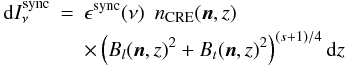
For the synchrotron emission (Rybicki & Lightman 1979) we write:

$\begin{array}{ccc}\mathrm{d}{\mathit{I}}_{\mathit{\nu }}^{\mathrm{sync}}& \mathrm{=}& {\mathit{ϵ}}^{\mathrm{sync}}\mathrm{\left(}\mathit{\nu }\mathrm{\right)}{\mathit{n}}_{\mathrm{CRE}}\mathrm{\left(}{n}\mathit{,z}\mathrm{\right)}\\ & & \mathrm{\times }{\mathrm{(}{\mathit{B}}_{\mathit{l}}\mathrm{(}{n}\mathit{,z}{\mathrm{)}}^{\mathrm{2}}\mathrm{+}{\mathit{B}}_{\mathit{t}}\mathrm{(}{n}\mathit{,z}{\mathrm{)}}^{\mathrm{2}}\mathrm{)}}^{\mathrm{(}\mathit{s}\mathrm{+}\mathrm{1}\mathrm{)}\mathit{/}\mathrm{4}}\mathrm{d}\mathit{z}\end{array}$(1)we obtain $\begin{array}{ccc}{\mathit{I}}_{\mathit{\nu }}^{\mathrm{sync}}\mathrm{\left(}{n}\mathrm{\right)}& \mathrm{=}& \int \mathrm{d}{\mathit{I}}_{\mathit{\nu }}^{\mathrm{sync}}\mathit{,}\\ {\mathit{Q}}_{\mathit{\nu }}^{\mathrm{sync}}\mathrm{\left(}{n}\mathrm{\right)}& \mathrm{=}& \int \mathrm{d}{\mathit{I}}_{\mathit{\nu }}^{\mathrm{sync}}\cos \mathrm{\left(}\mathrm{2}\mathit{\gamma }\mathrm{\right(}{n}\mathit{,z}\mathrm{\left)}\mathrm{\right)}{\mathit{p}}^{\mathrm{sync}}\mathit{,}\\ {\mathit{U}}_{\mathit{\nu }}^{\mathrm{sync}}\mathrm{\left(}{n}\mathrm{\right)}& \mathrm{=}& \mathrm{\int }\mathrm{d}{\mathit{I}}_{\mathit{\nu }}^{\mathrm{sync}}\sin \mathrm{\left(}\mathrm{2}\mathit{\gamma }\mathrm{\right(}{n}\mathit{,z}\mathrm{\left)}\mathrm{\right)}{\mathit{p}}^{\mathrm{sync}}\mathit{,}\end{array}$

where I, Q and U are the Stokes parameters and ϵ^sync(ν) is an emissivity term. γ is the polarization angle. B_n is the magnetic field component along the line of sight, n, and B_l and B_t the magnetic field components on a plane perpendicular to the line-of-sight. z is a 1D coordinate along the line-of-sight. s is the exponent of the power-law representing the energy distribution of relativistic electrons in the Galaxy. The polarization fraction, p^sync, is related to s, as follows ${\mathit{p}}^{\mathrm{sync}}\mathrm{=}\frac{\mathit{s}\mathrm{+}\mathrm{1}}{\mathit{s}\mathrm{+}\mathrm{7}\mathit{/}\mathrm{3}}\mathrm{·}$(5)

In the following we will assume a constant value of 3 for s so that the synchrotron emission will be proportional to the square of the perpendicular component of the Galactic magnetic field to the line of sight and p_sync = 0.75 (Rybicki & Lightman 1979).

Locally, the direction of polarization will be orthogonal to the magnetic field lines and to the line-of-sight. Then, the polarization angle γ is given by

$\begin{array}{ccc}\mathit{\gamma }\mathrm{\left(}{n}\mathit{,s}\mathrm{\right)}& \mathrm{=}& \frac{\mathrm{1}}{\mathrm{2}}\arctan \left(\frac{\mathrm{2}{\mathit{B}}_{\mathit{l}}\mathrm{\left(}{n}\mathit{,z}\mathrm{\right)}{\mathit{B}}_{\mathit{t}}\mathrm{\left(}{n}\mathit{,z}\mathrm{\right)}}{{\mathit{B}}_{\mathit{l}}^{\mathrm{2}}\mathrm{\left(}{n}\mathit{,z}\mathrm{\right)}\mathrm{-}{\mathit{B}}_{\mathit{t}}^{\mathrm{2}}\mathrm{\left(}{n}\mathit{,z}\mathrm{\right)}}\right)\mathrm{·}\end{array}$(6)

Thermal dust

For thermal dust emission we have

$\mathrm{d}{\mathit{I}}_{\mathit{\nu }}^{\mathrm{dust}}\mathrm{\left(}{n}\mathrm{\right)}\mathrm{=}{\mathit{ϵ}}^{\mathrm{dust}}\mathrm{\left(}\mathit{\nu }\mathrm{\right)}{\mathit{n}}_{\mathrm{dust}}\mathrm{\left(}{n}\mathit{,z}\mathrm{\right)}\mathrm{d}\mathit{z}$(7)we can write 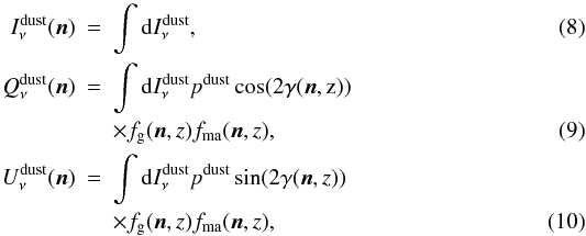$\begin{array}{ccc}{\mathit{I}}_{\mathit{\nu }}^{\mathrm{dust}}\mathrm{\left(}{n}\mathrm{\right)}& \mathrm{=}& \int \mathrm{d}{\mathit{I}}_{\mathit{\nu }}^{\mathrm{dust}}\mathit{,}\\ {\mathit{Q}}_{\mathit{\nu }}^{\mathrm{dust}}\mathrm{\left(}{n}\mathrm{\right)}& \mathrm{=}& \int \mathrm{d}{\mathit{I}}_{\mathit{\nu }}^{\mathrm{dust}}{\mathit{p}}^{\mathrm{dust}}\cos \mathrm{\left(}\mathrm{2}\mathit{\gamma }\mathrm{\right(}{n}\mathit{,}\mathrm{z}\mathrm{\left)}\mathrm{\right)}\\ & & \mathrm{\times }{\mathit{f}}_{\mathrm{g}}\mathrm{\left(}{n}\mathit{,z}\mathrm{\right)}{\mathit{f}}_{\mathrm{ma}}\mathrm{\left(}{n}\mathit{,z}\mathrm{\right)}\mathit{,}\\ {\mathit{U}}_{\mathit{\nu }}^{\mathrm{dust}}\mathrm{\left(}{n}\mathrm{\right)}& \mathrm{=}& \int \mathrm{d}{\mathit{I}}_{\mathit{\nu }}^{\mathrm{dust}}{\mathit{p}}^{\mathrm{dust}}\sin \mathrm{\left(}\mathrm{2}\mathit{\gamma }\mathrm{\right(}{n}\mathit{,z}\mathrm{\left)}\mathrm{\right)}\\ & & \mathrm{\times }{\mathit{f}}_{\mathrm{g}}\mathrm{\left(}{n}\mathit{,z}\mathrm{\right)}{\mathit{f}}_{\mathrm{ma}}\mathrm{\left(}{n}\mathit{,z}\mathrm{\right)}\mathit{,}\end{array}$where ϵ^dust is the dust emissivity, p^dust is the polarization fraction, γ is the polarization angle, and, f_g and f_ma are polarization suppression factors (see below). The polarization fraction p^dust will be considered a free parameter in the analysis.

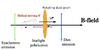Fig. 3 Schematic view of the polarization direction of the Galactic synchrotron and dust thermal emissions as functions of the Galactic magnetic field direction.

As discussed before, dust grains in the ISM are oblates and will align their large axis (see Fig. 3) perpendicularly to the magnetic field lines (Davis & Greenstein 1951; Lazarian 1995; Lazarian et al. 1997; Lazarian 2009). Therefore, the polarization direction for thermal dust emission will be perpendicular both to the magnetic field lines and the line-of-sight as was already the case for the synchrotron emission. Then, the polarization angle γ will be the same for the synchrotron and thermal dust emissions. However, as the dust grains rotate with their spin axis parallel to the magnetic field, we also need to account for a geometrical suppression factor. For instance, if the magnetic field lines are parallel to the line-of-sight, we expect the dust polarized emission to be fully suppressed. The suppression factor can be expressed as f_g = sin²(α) where α is the angle between the magnetic field lines and the line-of-sight. By construction, we observe that γ and α are the same angle. The process of alignment of the dust grains with the magnetic field is very complex (Mathis 1986; Goodman & Whittet 1995; Lazarian 1995; Lazarian et al. 1997; Lazarian 2009) and its accurate representation is out of the scope of this paper. Then, to account for misalignment between the dust grains and the magnetic field lines we define an empirical factor f_ma. The exact form of this factor is unknown but we have empirically observed that the geometrical suppression seems to be more important than expected for the Archeops data. Therefore, we have taken f_ma to be  ∝ sin(α). We have observed that the results presented in this paper are robusts with respect to the parameter.

3.1. Matter density model

In galactocentric cylindrical coordinates (r,z,φ) the relativistic electrons density distribution can be written as (see Drimmel & Spergel 2001) 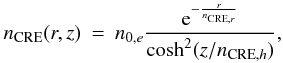$\begin{array}{ccc}{\mathit{n}}_{\mathrm{CRE}}\mathrm{\left(}\mathit{r,z}\mathrm{\right)}& \mathrm{=}& {\mathit{n}}_{\mathrm{0}\mathit{,e}}\frac{{\mathrm{e}}^{\mathrm{-}\frac{\mathit{r}}{{\mathit{n}}_{\mathrm{CRE}\mathit{,r}}}}}{{\cosh }^{\mathrm{2}}\mathrm{(}\mathit{z}\mathit{/}{\mathit{n}}_{\mathrm{CRE}\mathit{,h}}\mathrm{)}}\mathit{,}\end{array}$(11)

where n_CRE,h defines the width of the distribution vertically and is set to 1 kpc in the following. n_CRE,r defines the distribution radially and it is a free parameter of the model. Notice that we expect these two parameters to be strongly correlated, hence we decided to fix one of them as in previous analyses (Sun et al. 2008; Jaffe et al. 2010).

The density distribution of dust grains in the Galaxy is poorly known and we therefore elect to describe it in the same way as for relativistic electrons:

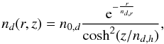${\mathit{n}}_{\mathit{d}}\mathrm{\left(}\mathit{r,z}\mathrm{\right)}\mathrm{=}{\mathit{n}}_{\mathrm{0}\mathit{,d}}\frac{{\mathrm{e}}^{\mathrm{-}\frac{\mathit{r}}{{\mathit{n}}_{\mathit{d,r}}}}}{{\cosh }^{\mathrm{2}}\mathrm{(}\mathit{z}\mathit{/}{\mathit{n}}_{\mathit{d,h}}\mathrm{)}}\mathit{,}$(12)

where n_d,r and n_d,h are the radial and vertical widths of the distribution. In the following we set them to 3 and 1 kpc respectively. We have tested different values of these two parameters and found no impact on the final results.

3.2. Galactic magnetic field model

According to observations many spiral galaxies over a range of redshifts show evidences of a large scale magnetic field with intensity of few μG, and a direction spatially correlated with the spiral arms (Sofue et al. 1986; Beck et al. 1996; Wielebinski 2005). For our Galaxy, the magnetic field direction also seems to follow the spiral arms but with a complex spatial distribution (Wielebinski 2005; Han et al. 2006; Beck 2006). Indeed, there are hints for local reversals in the field direction and radial dependency of the intensity (Han et al. 2006; Beck 2001). Pulsar Faraday rotation measurements (Han et al. 2004, 2006; Sofue et al. 1986; Brown et al. 2007) have been used to fit the Galactic large-scale magnetic field with various models including both axisymmetric and bisymmetric forms, or a field that reverses in the inter-arm regions, etc. Pulsar Faraday rotation measurements also indicate the presence of a turbulent component of the magnetic field (Han et al. 2004). As discussed in Jaffe et al. (2010) the turbulent Galactic magnetic field can be separated into an isotropic and an anisotropic component. The latter, also called ordered random component, will be not considered in this paper because it cannot be distinguished from the large-scale magnetic field when studying polarization intensity only.

3.2.1. Large-scale magnetic field

In the following we consider a modified logarithmic spiral (MLS) model of the large-scale magnetic field based on the Wmap team model presented in Page et al. (2007). It assumes a logarithmic spiral to mimic the shape of the spiral arms (Sofue et al. 1986) to which we have added a vertical component. In galactocentric cylindrical coordinates (r,z,Φ) it reads

$\begin{array}{ccc}{B}\mathrm{\left(}{r}\mathrm{\right)}& \mathrm{=}& {\mathit{B}}_{\mathrm{reg}}\mathrm{\left(}{r}\mathrm{\right)}\mathrm{\left[}\cos \mathrm{\right(}\mathit{\phi }\mathrm{+}\mathit{\beta }\mathrm{\left)}\ln \left(\frac{\mathit{r}}{{\mathit{r}}_{\mathrm{0}}}\right)\sin \mathrm{\right(}\mathit{p}\mathrm{\left)}\cos \mathrm{\right(}\mathit{\chi }\mathrm{)}{u}\mathrm{r}\\ & & \mathrm{-}\cos \mathrm{(}\mathit{\phi }\mathrm{+}\mathit{\beta }\mathrm{)}\ln \left(\frac{\mathit{r}}{{\mathit{r}}_{\mathrm{0}}}\right)\cos \mathrm{\left(}\mathit{p}\mathrm{\right)}\cos \mathrm{\left(}\mathit{\chi }\mathrm{\right)}{u}\mathit{\phi }\\ & & \mathrm{+}\sin \mathrm{\left(}\mathit{\chi }\mathrm{\right)}{u}\mathrm{z}\mathrm{]}\mathit{,}\end{array}$(13)where p is the pitch angle and β = 1/tan(p). r₀ is the radial scale and χ(r) = χ₀(r)(z/z₀) is the vertical scale. Following Taylor & Cordes (1993) we restrict our model to the range 3 < r < 20 kpc. The lower limit is set to avoid the center of the Galaxy for which the physics is poorly constrained and the model diverges. The intensity of the regular field is fixed using pulsar Faraday rotation measurements by Han et al. 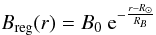(2006)${\mathit{B}}_{\mathrm{reg}}\mathrm{\left(}\mathit{r}\mathrm{\right)}\mathrm{=}{\mathit{B}}_{\mathrm{0}}{\mathrm{e}}^{\mathrm{-}\frac{\mathit{r}\mathrm{-}{\mathit{R}}_{\mathrm{\odot }}}{{\mathit{R}}_{\mathit{B}}}}$(14)

where the large-scale field intensity at the Sun position is B₀ = 2.1 ± 0.3   μG and R_B = 8.5 ± 4.7 kpc. The distance between the Sun and the Galactic center, R_⊙ is set to 8 kpc (Eisenhauer et al. 2003; Reid & Brunthaler 2005).

We also study the spiral model of Stanev (1997); Sun et al. (2008), hereafter ASS. In cylindrical coordinates it is given by

$\begin{array}{ccc}{\mathit{B}}_{\mathit{r}}^{\mathit{D}}& \mathrm{=}& {\mathit{D}}_{\mathrm{1}}\mathrm{\left(}\mathit{r,}\mathrm{\Phi }\mathit{,z}\mathrm{\right)}{\mathit{D}}_{\mathrm{2}}\mathrm{\left(}\mathit{r,}\mathrm{\Phi }\mathit{,z}\mathrm{\right)}\sin \mathrm{\left(}\mathit{p}\mathrm{\right)}\\ {\mathit{B}}_{\mathrm{\Phi }}^{\mathit{D}}& \mathrm{=}& \mathrm{-}{\mathit{D}}_{\mathrm{1}}\mathrm{\left(}\mathit{r,}\mathrm{\Phi }\mathit{,z}\mathrm{\right)}{\mathit{D}}_{\mathrm{2}}\mathrm{\left(}\mathit{r,}\mathrm{\Phi }\mathit{,z}\mathrm{\right)}\cos \mathrm{\left(}\mathit{p}\mathrm{\right)}\\ {\mathit{B}}_{\mathit{z}}^{\mathit{D}}& \mathrm{=}& \mathrm{0}\end{array}$

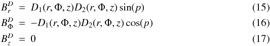
where D₁ accounts for the spatial variations of the field and D₂ for asymmetries or reversals in the direction. The pitch angle is defined as for the MLS model described above. D₁(r,z) is given by

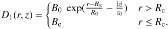${\mathit{D}}_{\mathrm{1}}\mathrm{\left(}\mathit{r,z}\mathrm{\right)}\mathrm{=}\{\begin{array}{c}\\ & \mathit{r}\mathit{>}{\mathit{R}}_{\mathrm{c}}\\ & \mathit{r}\mathrm{\le }{\mathit{R}}_{\mathrm{c}}\mathit{.}\end{array}$(18)

where R_⊙ is the distance of the Sun to the center of the Galaxy and it is set to 8 kpc as before. R_c is a critical radius and it is set to 5 kpc following the ASS+RING model in Sun et al. (2008). In the same way R₀ is fixed to 10 kpc, B₀ to 6 μG and B_c to 2 μG. The field reversals are as in Sun et al. (2008) although it is important to notice that the synchrotron and thermal dust polarized emissions depend only on the orientation and not on the sign of the magnetic field and therefore are not sensitives to field reversals.

3.2.2. Turbulent component

In addition to the large-scale Galactic magnetic field, Faraday rotation measurements on pulsars in our vicinity have revealed a turbulent component on scales smaller than a few hundred pc (Lyne & Smith 1989). Moreover it seems to be present on large angular scales (Han et al. 2004) with an amplitude estimated to be of the same order of magnitude as that of the regular one (Han et al. 2006). The magnetic energy E_B(k) associated with the turbulent component is well described by a power spectrum of the form (Han et al. 2004, 2006) 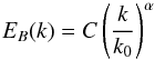${\mathit{E}}_{\mathit{B}}\mathrm{\left(}\mathit{k}\mathrm{\right)}\mathrm{=}\mathit{C}{\left(\frac{\mathit{k}}{{\mathit{k}}_{\mathrm{0}}}\right)}^{\mathit{\alpha }}$(19)

where α =  − 0.37 and C = (6.8 ± 0.3) × 10^-13   erg   cm^-3   kpc. As discussed before, we only consider here an isotropic random Galactic magnetic field, modelling an ordered component is beyond the scope of this paper.

3.2.3. Final model

Finally the total magnetic Galactic field B_tot(r) can be written as

${B}\mathrm{tot}\mathrm{\left(}{r}\mathrm{\right)}\mathrm{=}{B}\mathrm{reg}\mathrm{\left(}{r}\mathrm{\right)}\mathrm{+}{B}\mathrm{turb}\mathrm{\left(}{r}\mathrm{\right)}$(20)

where B_reg(r) is the regular component, either MLS or ASS, and B_turb(r) is the turbulent one. We define A_turb as the relative intensity of the turbulent component with respect to the regular one and it is a free parameter of the model. The turbulent component is computed from a 3D random realization of the power law spectrum presented above over a box of 512³ points of 56 pc resolution.

In this paper we do not consider the halo component presented by Sun et al. (2008); Jansson et al. (2009) as relativistic electrons and dust grains are not expected to be concentrated on the halo.

3.3. Emissivity model in polarization

As discussed in the previous section, the polarized emission in the 23 GHz Wmap data shows complex structures both on the Galactic plane and in local high Galactic latitude structures such as the north polar spur (Page et al. 2007). An accurate representation of this complexity cannot be achieved using our simplified model. A similar degree of complexity is observed in the 353 GHz polarization maps although the morphology of the structures is rather different. To account for this, the Q and U estimated for synchrotron and thermal dust models are corrected using intensity templates of these components extrapolated to the observation frequencies (23 and 353 GHz) using constant spectral indices.

For the synchrotron emission we have

$\begin{array}{ccc}{\mathit{Q}}_{\mathrm{s}}& \mathrm{=}& {\mathit{I}}_{\mathrm{Has}}{\left(\frac{\mathit{\nu }}{\mathrm{0.408}}\right)}^{{\mathit{\beta }}_{\mathrm{s}}}\frac{{\mathit{Q}}_{\mathit{\nu }}^{\mathrm{sync}}}{{\mathit{I}}_{\mathit{\nu }}^{\mathrm{sync}}}\mathit{,}\\ {\mathit{U}}_{\mathrm{s}}& \mathrm{=}& {\mathit{I}}_{\mathrm{Has}}{\left(\frac{\mathit{\nu }}{\mathrm{0.408}}\right)}^{{\mathit{\beta }}_{\mathrm{s}}}\frac{{\mathit{U}}_{\mathit{\nu }}^{\mathrm{sync}}}{{\mathit{I}}_{\mathit{\nu }}^{\mathrm{sync}}}\mathit{,}\end{array}$

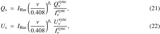
where I_Has is the reference map in intensity constructed from the 408 MHz all sky continuum survey (see Sect. 2.1.1) after subtraction of the free-free emission and ν is the frequency of observation. Notice that we do not use the synchrotron MEM intensity map at 23 GHz (Hinshaw et al. 2007) as a synchrotron template to avoid any possible spinning dust contamination (the Wmap team made no attempt to fit for the latter component). The spectral index β_s used to extrapolate maps at various frequencies is a free parameter of the model.

For the thermal dust emission we write 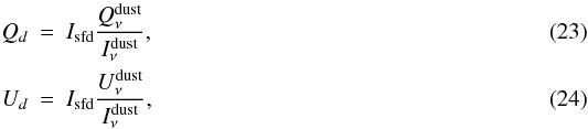$\begin{array}{ccc}{\mathit{Q}}_{\mathit{d}}& \mathrm{=}& {\mathit{I}}_{\mathrm{sfd}}\frac{{\mathit{Q}}_{\mathit{\nu }}^{\mathrm{dust}}}{{\mathit{I}}_{\mathit{\nu }}^{\mathrm{dust}}}\mathit{,}\\ {\mathit{U}}_{\mathit{d}}& \mathrm{=}& {\mathit{I}}_{\mathrm{sfd}}\frac{{\mathit{U}}_{\mathit{\nu }}^{\mathrm{dust}}}{{\mathit{I}}_{\mathit{\nu }}^{\mathrm{dust}}}\mathit{,}\end{array}$where I_sfd is the reference map in intensity at 353 GHz generated using model 8 from Finkbeiner et al. (1999).

We compute the I, Q and U maps for synchrotron and thermal dust with a modified version of the Hammurabi code (Waelkens et al. 2009). Each map is generated by integrating in 100 steps along each line-of-sight defined by the HEALPix N_side = 128 pixel centres. The integration continues out to 25 kpc from the observer situated 8.5 kpc from the Galactic centre.

4. Galactic-profiles comparison

4.1. Galactic-profiles description

In order to compare the models of Galactic polarized emissions to the available data, we compute Galactic longitude and latitude profiles for the models and for the data in temperature and polarization using the sets of latitude and longitude bands defined in Table 1. In both cases, we use bins of longitude of 2.5°. In the following discussions, we only consider Galactic latitude profiles because equivalent results are obtained with the longitudinal profiles.

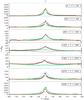Fig. 4 Galactic profiles in temperature at 408 MHz built using the Haslam data (black) and the model of synchrotron emission with MLS for various values of the pitch angle p  −70,  −30 and 50 degrees (from green to red).

We compute error bars including intrinsic instrumental uncertainties and the extra variance induced by the presence of a turbulent component. The latter is estimated from the RMS within each of the latitude bins following Jansson et al. (2009). For the 408 MHz all sky continuum survey we account for intrinsic uncertainties due to the 10% calibration errors described in Sect. 2. For the Wmap 23 GHz data we have computed 600 realizations of Gaussian noise maps from the number of hits per pixel and the sensitivity per hit given on the Wmap LAMBDA web site. We have computed Galactic latitude profiles in polarization for these simulated maps and estimated intrinsic errors from the standard deviation within each latitude bin. For the Archeops data we use the noise simulations discussed in Macías-Pérez et al. (2007) and proceed as for the Wmap data.

Galactic latitude profiles are computed for a grid of models obtained by varying the pitch angle, p, the turbulent component amplitude, A_turb, the dust fraction of polarization, p^dust, the radial scale for the synchrotron emission, n_CRE,r, and the synchrotron spectral index, β_s. The latter is assumed to be spatially constant on the sky. Dealing with a more realistic varying spectral index (see Kogut et al. 2007; La Porta et al. 2008 for detailed studies) is beyond the scope of this paper. However, we ensured that this hypothesis does not impact the results for the other free parameters in the model. Indeed, we produced simulated Wmap observations at 23 GHz with spatially varying synchrotron spectral index and analysed them assuming a constant one. No significant bias was observed for any of the other parameters and the error bars were compatibles with those in the cases of a constant spectral index.

The range and binning step considered for each of the above parameters are given in Table 2. All the other parameters of the models of the Galactic magnetic field and matter density are fixed to values proposed in Sect. 3. Notice that to be able to compare the dust models to the Archeops 353 GHz data, the simulated maps are multiplied by a mask to account for the Archeops incomplete sky coverage.

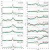Fig. 5 Galactic profiles in polarization Q and U at 23 GHz built with the five-year WMAP data (black) and the model of synchrotron emission with MLS magnetic field for various values of the pitch angle p,  −70,  −30 and 50 degrees (from green to red).

Figure 4 shows in black Galactic latitude profiles in temperature for the 408 MHz all sky continuum survey with error bars computed as discussed above. In color, we show for comparison the expected galactic diffuse synchrotron emission from the MLS Galactic magnetic field model for various values of the pitch angle p from  − 80 to 80 degrees in steps of 20 degrees. In Fig. 5 we present the polarization Galactic latitude profiles for the Wmap 23 GHz data (black) and the expected polarized diffuse synchrotron emission for the previous MLS models (color). Finally, Fig. 6 shows the polarization Galactic latitude profiles for the 353 GHz Archeops data (black) compared to the same MLS models (color). From these figures we can see that the current available data do have discriminative power between the different models and therefore a likelihood analysis is justified.

Fig. 6 Galactic profiles in temperature and polarization Q and U at 353 GHz with the ARCHEOPS data (black) and for various values of the pitch angle p,  − 70,  − 30 and 50 degrees, for the model in polarization of thermal dust emission with MLS magnetic field (from green to red).

4.2. Likelihood analysis

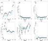Fig. 7 From left to right and from top to bottom: power spectra ${\mathit{C}}_{\mathit{l}}^{\mathrm{TT}}$,${\mathit{C}}_{\mathit{l}}^{\mathrm{EE}}$,${\mathit{C}}_{\mathit{l}}^{\mathrm{BB}}$,${\mathit{C}}_{\mathit{l}}^{\mathrm{TE}}$,${\mathit{C}}_{\mathit{l}}^{\mathrm{TB}}$,${\mathit{C}}_{\mathit{l}}^{\mathrm{EB}}$ at 23 GHz built with the 5-year Wmap data (black) and the model of synchrotron emission with MLS magnetic field for the best fit model parameters, excluding the Galactic region defined by  | b |  < 5°.

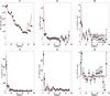Fig. 8 From left to right and from top to bottom: power spectra ${\mathit{C}}_{\mathit{l}}^{\mathrm{TT}}$,${\mathit{C}}_{\mathit{l}}^{\mathrm{EE}}$,${\mathit{C}}_{\mathit{l}}^{\mathrm{BB}}$,${\mathit{C}}_{\mathit{l}}^{\mathrm{TE}}$,${\mathit{C}}_{\mathit{l}}^{\mathrm{TB}}$,${\mathit{C}}_{\mathit{l}}^{\mathrm{EB}}$ at 353 GHz computed from Archeops data (black) and the model of thermal dust emission with MLS magnetic field for the best fit model parameters (red) for the full sky.

The data and model Galactic latitude profiles are compared using a likelihood analysis where the total likelihood function is obtained from ${\mathrm{ℒ}}_{\mathrm{tot}}\mathrm{=}{\mathrm{\Pi }}_{\mathit{d}\mathrm{=}\mathrm{1}}^{\mathrm{3}}{\mathrm{ℒ}}_{\mathit{d}}$(25)where for each of the 3 data sets described above the log-likelihood function is given by

$\mathrm{-}\log {\mathrm{ℒ}}_{\mathit{d}}\mathrm{=}\sum _{\mathit{i}}\sum _{\mathit{j}\mathrm{=}\mathrm{0}}^{{\mathit{N}}_{\mathrm{lon}}\mathrm{-}\mathrm{1}}\sum _{\mathit{k}\mathrm{=}\mathrm{0}}^{{\mathit{N}}_{\mathrm{lat}}\mathrm{-}\mathrm{1}}\frac{\mathrm{(}{\mathit{D}}_{\mathit{i,j,k}}^{\mathit{d}}\mathrm{-}{\mathit{M}}_{\mathit{i,j,k}}^{\mathit{d}}{\mathrm{)}}^{\mathrm{2}}}{{{\mathit{\sigma }}_{\mathit{i,j,k}}^{\mathit{d}}}^{\mathrm{2}}}$(26)

where i represents the polarization state meaning intensity only for the 408 MHz all-sky survey, and, Q and U polarization for the 23 GHz WMAP and 353 GHz Archeops data. j and k represent the longitude bands and latitude bins respectively. ${\mathit{D}}_{\mathit{i,j,k}}^{\mathit{d}}$ and ${\mathit{M}}_{\mathit{i,j,k}}^{\mathit{d}}$ correspond to the data set d and model for the i polarization state, j longitude band and k latitude bin, respectively. ${\mathit{\sigma }}_{\mathit{i,j,k}}^{\mathit{d}}$ is the error bar associated with ${\mathit{M}}_{\mathit{i,j,k}}^{\mathit{d}}$.

Table 3 presents the best-fit parameters for the three individual data sets described above and also for their combination (labeled All in the table). Results are presented both for the MLS and ASS models of the Galactic magnetic field. The best-fit values for the pitch angle, p, are in agreement within 1-σ error bars for the three data sets. From the full data set, we can conclude that the pitch angle favoured by the data is around  − 30 degrees with error bars of the order of 10 to 20 degrees both for the MLS and ASS models. The final error bars on this parameter are in agreement with the dispersion observed from different data sets, except for the Archeops ASS case. These results are compatible with the pitch angle values presented in Sun et al. (2008); Page et al. (2007); Miville-Deschênes et al. (2008). The relative amplitude of the turbulent component, A_turb, is poorly constrained and the data do not seem to favour a strong turbulent component either in the case of MLS or ASS models. However, our results are compatibles with the ones presented in Sun et al. (2008); Miville-Deschênes et al. (2008); Han et al. (2004, 2006) at the 2-σ level. The electron density radial scale, n_CRE,r, is poorly constrained by the data both for MLS and ASS models although our results are compatible with those of Sun et al. (2008). We also tested the possibility of a local contribution to the electronic density as proposed by Sun et al. (2008). We found that adding this local component improves neither the fit nor the constraint on the radial scale. The best-fit value for the spectral index of the synchrotron emission seems to be significantly lower than the one in Sun et al. (2008); Page et al. (2007). This may due to differences between the intensity template. Notice that we rescale the polarization intensity using the 408 MHz all sky continuum survey to obtain a more realistic model. Finally, we observe that the constraints on the polarization fraction for dust, p^dust are weak but they are in agreement with the results in Ponthieu et al. (2005).

4.3. Temperature and polarization angular power spectra

Using the best-fit parameters of the MLS model, p =  − 30.0°, A_turb = 0.0, n_CRE,r = 4 and β_s =  − 3.4, we have constructed simulated maps of the sky at 408 MHz and 23 and 353 GHz. Notice that for A_turb we only had an upper-limit from the analysis and therefore, we have decided to set it equal to zero to maximize the possible foreground emissions in the following study. These maps are shown on right-hand side of Figs. 2.1.1 and 2. Although for the Galactic profiles the fit can be considered relatively good, the fake temperature map at 408 MHz looks very different from the 408 MHz all-sky survey map (left side of the plot), in particular at the North Polar Spur (Wolleben 2007), as no local structures were included in the model. This supports a posteriori our correction of the polarization synchrotron model using an intensity template as presented in Sect. 3. In Q and U polarization, the 23 GHz simulated maps seem to reproduce qualitatively the structures observed in the Wmap data (left side of the plot). However in temperature the model and the data are very different as we have not accounted for spatially variable synchrotron spectra nor for any extra component as discussed in Page et al. (2007); Kogut et al. (2007); Miville-Deschênes et al. (2008). Finally, the model of thermal dust emission is able to reproduce qualitatively the Archeops data at 353 GHz.

I, Q and U maps can be decomposed in spherical harmonics leading to the ${\mathit{a}}_{\mathit{\ell ,m}}^{\mathit{T}}$, ${\mathit{a}}_{\mathit{\ell ,m}}^{\mathit{E}}$ and ${\mathit{a}}_{\mathit{\ell ,m}}^{\mathit{B}}$ coefficients. The auto and cross-correlation of the latter form the 9 temperature and polarization angular power spectra, ${\mathit{C}}_{\mathit{\ell }}^{\mathit{XY}}\mathrm{=}\mathrm{⟨}{\mathit{a}}_{\mathit{\ell ,m}}^{\mathit{X}}\mathit{,}{\mathit{a}}_{\mathit{\ell ,m}}^{\mathit{Y}}\mathrm{⟩}$, where X and Y can be either T, E or B. Figures 7 and 8 show the temperature and polarization angular power spectra for the 23 GHz Wmap and 353 GHZ Archeops data compared to the best-fit MLS model for synchrotron and dust, respectively. As discussed before, the temperature auto power spectrum of the 23 GHz data is very different from the model as no extra components in temperature were considered. However in polarization we have qualitatively a good agreement. However, we clearly observe that the model does not account for all the observed emission. At 353 GHz the agreement between the data and the model qualitatively and quantitatively is good. For polarization most of the data samples at less than 3-σ from the model. In temperature the model is not as accurate as in polarization but we notice that the fitting was restricted to polarization data only.

5. Galactic foreground contamination to the CMB measurements by the PLANCK satellite

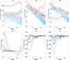Fig. 9 From left to right and from top to bottom: power spectra ${\mathit{C}}_{\mathit{l}}^{\mathrm{TT}}$,${\mathit{C}}_{\mathit{l}}^{\mathrm{EE}}$,${\mathit{C}}_{\mathit{l}}^{\mathrm{BB}}$,${\mathit{C}}_{\mathit{l}}^{\mathrm{TE}}$,${\mathit{C}}_{\mathit{l}}^{\mathrm{TB}}$,${\mathit{C}}_{\mathit{l}}^{\mathrm{EB}}$ at 100 GHz for the model of Galactic polarized emission applying a Galactic cut of  | b |  < 15° (black) 30° (blue) and 40° (cyan). The dashed curves indicate the 1-σ error bars in the models. We compared them to the expected CMB ones (red) for the Wmap best-fit ΛCDM model (Komatsu et al. 2009) to which we added a tensor component assuming a tensor to scalar ratio of 0.1.

We can use the best-fit model of polarized synchrotron and dust emissions to estimate the polarized foregrounds contamination to the CMB at the Planck satellite observation frequencies. Notice that the aim of this section is not to obtain an accurate template of the polarized Galactic foreground emissions to be subtracted from the Planck data for subsequent CMB analysis. However, we are interested in comparing the predicted foregrounds contribution to the CMB emission.

For this purpose, we have produced simulated maps of the Galactic polarized foreground emissions using the best-fit model parameters for each of the Planck CMB frequencies, 70, 100, 143 and 217 GHz. The thermal dust polarized emission have been extrapolated using a constant spectral index of 2.0 in antenna temperature. We have computed the temperature and polarization power spectra of these maps and compared them to the expected CMB ones for the Wmap best-fit ΛCDM model (available on the LAMBDA website) to which we added a tensor component assuming a tensor to scalar ratio of 0.1. Note that neither noise, systematics nor resolution effects are considered.

Figure 9 shows these power spectra at 100 GHz. The expected CMB signal is represented in red. The polarized diffuse foreground emissions for Galactic latitude cuts of  |b|  < 15°, 30° and 40° are shown as solid black, blue and cyan lines, respectively. 1-σ errors in the model are represented as dashed lines. In temperature, the CMB ${\mathit{C}}_{\mathit{l}}^{\mathrm{TT}}$ dominates at all the angular scales considered as could be expected from the Wmap and Archeops data. For polarization, the CMB ${\mathit{C}}_{\mathit{l}}^{\mathrm{EE}}$ dominates at high ℓ values but we observe significant foreground contamination at the lowest ℓ values (ℓ < 20). In the same way, the CMB ${\mathit{C}}_{\mathit{l}}^{\mathrm{TE}}$ dominates at 100 GHz but for very low ℓ values. However, the CMB ${\mathit{C}}_{\mathit{l}}^{\mathrm{BB}}$ is significantly smaller than the foreground contribution at all the angular scales considered even for such a large value of the tensor to scalar ratio. The CMB ${\mathit{C}}_{\mathit{l}}^{\mathrm{TB}}$ and ${\mathit{C}}_{\mathit{l}}^{\mathrm{EB}}$ are expected for most cosmological models to be null and therefore, the foregrounds contribution dominates the signal. These results are consistent with previous estimates by La Porta et al. (2006) who considered only synchrotron emission and with those of Ponthieu et al. (2005) who modeled only the dust emission.

As the Galactic polarized foreground emissions seem to dominate the observed emission at the Planck CMB frequencies, special care should be taken when estimating the CMB emission using standard template subtraction techniques and component separation algorithms. The assessment of the final errors is crucial and it is likely that models of the polarized foreground emissions such as those presented in this paper can be of substantial help in this task.

6. Summary and conclusions

We have presented in this paper a detailed study of the polarized Galactic foregrounds due to diffuse synchrotron and thermal dust emissions. We have constructed coherent models of these two foregrounds based on a 3D representation of the Galactic magnetic field and of the distributions of relativistic electrons and dust grains in the Galaxy. For the Galactic magnetic field we have assumed a large-scale regular component plus a turbulent one. The relativistic electrons and dust grains distributions have been modeled with exponentials peaking at the Galactic center. From these analysis we have been able to study the main parameters of the models, the magnetic field pitch angle, p, the radial width of the relativistic electron distribution, h_er, the relative amplitude of the turbulent component, A_turb and spectral index of the synchrotron emission β_s. We have been able to set constraints only on the pitch angle and the synchrotron spectral index. An upper limit on the relative amplitude of the turbulent component is obtained although the data seems to prefer no turbulence at large angular scales. With the current data we are not able to constrain the radial width of the relativistic electron distribution. Notice that our constraints are compatible with those in the literature.

Using the best-fit parameters we have constructed maps in temperature and polarization for the synchrotron and thermal dust emissions at 23 and 353 GHz and compared them to the Wmap and Archeops data at the same frequencies. We find good agreement between the data and the model. However, when comparing the temperature and polarization power spectra for the data and model maps, we observe that the synchrotron emission model is not realistic enough. For dust the model seems to reproduce the data in better detail, but it is important to realize that the errors on the Archeops data are much larger.

From this, we can conclude that the models presented in this paper cannot be used for direct subtraction of polarized foregrounds for CMB purposes. However, they can be of great help in estimating the impact of the polarized Galactic foreground emissions on the reconstruction of the CMB polarized power spectra. Indeed, we have extrapolated the expected polarized Galactic foreground emissions to the Planck CMB frequencies, 70, 100, 143 and 217 GHz and found that they dominate the emissions at low ℓ, values where the signature of important physical processes such as reionization are expected in the polarized CMB power spectra. Furthermore, the Galactic polarized foreground emissions seem to dominate the B modes for which we expect a unique signature from primordial gravitational waves. Because of this, we propose the use of models similar to those presented in this paper to assess the errors in the reconstruction of the CMB emission when using template subtraction techniques or component separation algorithms.

References

All Tables

All Figures

	Fig. 1 Intensity maps at 408 MHz in KRJ units for the Haslam data (left) and built with the model of synchrotron emission with an MLS magnetic field for the best fit model parameters (right).
In the text

Fig. 2 Form top to bottom: maps in intensity, I, and polarization Q and U at 23 GHz for the WMAP 5-year data (left) and the model of synchrotron emission with MLS magnetic field for the best fit model parameters (right) and at 353 GHz for the Archeops data (left) and the model of thermal dust emission with MLS magnetic field for the best fit model parameters (right). The 353 GHz maps are rotated by 180° for better visualization. All the maps are in KRJ units.

In the text

	Fig. 3 Schematic view of the polarization direction of the Galactic synchrotron and dust thermal emissions as functions of the Galactic magnetic field direction.
In the text

	Fig. 4 Galactic profiles in temperature at 408 MHz built using the Haslam data (black) and the model of synchrotron emission with MLS for various values of the pitch angle p  −70,  −30 and 50 degrees (from green to red).
In the text

	Fig. 5 Galactic profiles in polarization Q and U at 23 GHz built with the five-year WMAP data (black) and the model of synchrotron emission with MLS magnetic field for various values of the pitch angle p,  −70,  −30 and 50 degrees (from green to red).
In the text

	Fig. 6 Galactic profiles in temperature and polarization Q and U at 353 GHz with the ARCHEOPS data (black) and for various values of the pitch angle p,  − 70,  − 30 and 50 degrees, for the model in polarization of thermal dust emission with MLS magnetic field (from green to red).
In the text

Fig. 7 From left to right and from top to bottom: power spectra ${\mathit{C}}_{\mathit{l}}^{\mathrm{TT}}$,${\mathit{C}}_{\mathit{l}}^{\mathrm{EE}}$,${\mathit{C}}_{\mathit{l}}^{\mathrm{BB}}$,${\mathit{C}}_{\mathit{l}}^{\mathrm{TE}}$,${\mathit{C}}_{\mathit{l}}^{\mathrm{TB}}$,${\mathit{C}}_{\mathit{l}}^{\mathrm{EB}}$ at 23 GHz built with the 5-year Wmap data (black) and the model of synchrotron emission with MLS magnetic field for the best fit model parameters, excluding the Galactic region defined by  | b |  < 5°.

In the text

Fig. 8 From left to right and from top to bottom: power spectra ${\mathit{C}}_{\mathit{l}}^{\mathrm{TT}}$,${\mathit{C}}_{\mathit{l}}^{\mathrm{EE}}$,${\mathit{C}}_{\mathit{l}}^{\mathrm{BB}}$,${\mathit{C}}_{\mathit{l}}^{\mathrm{TE}}$,${\mathit{C}}_{\mathit{l}}^{\mathrm{TB}}$,${\mathit{C}}_{\mathit{l}}^{\mathrm{EB}}$ at 353 GHz computed from Archeops data (black) and the model of thermal dust emission with MLS magnetic field for the best fit model parameters (red) for the full sky.

In the text

Fig. 9 From left to right and from top to bottom: power spectra ${\mathit{C}}_{\mathit{l}}^{\mathrm{TT}}$,${\mathit{C}}_{\mathit{l}}^{\mathrm{EE}}$,${\mathit{C}}_{\mathit{l}}^{\mathrm{BB}}$,${\mathit{C}}_{\mathit{l}}^{\mathrm{TE}}$,${\mathit{C}}_{\mathit{l}}^{\mathrm{TB}}$,${\mathit{C}}_{\mathit{l}}^{\mathrm{EB}}$ at 100 GHz for the model of Galactic polarized emission applying a Galactic cut of  | b |  < 15° (black) 30° (blue) and 40° (cyan). The dashed curves indicate the 1-σ error bars in the models. We compared them to the expected CMB ones (red) for the Wmap best-fit ΛCDM model (Komatsu et al. 2009) to which we added a tensor component assuming a tensor to scalar ratio of 0.1.

In the text

References

- Battistelli, E., Rebolo, R., Rubinõ Martin, J., et al. 2006, ApJ, 645, 141 [Google Scholar]
- Baumann, D. E. 2009, in AIP Conf. Proc., 1141 [Google Scholar]
- Beck, R. 2001, Space Sci. Rev., 99, 243 [NASA ADS] [CrossRef] [Google Scholar]
- Beck, R. 2006, in Proceedings of Polarization 2005 (EAS PS) [Google Scholar]
- Beck, R., Brandenburg, A., Moss, D., Shukurov, A., & Sokoloff, D. 1996, ARA&A, 34, 155 [NASA ADS] [CrossRef] [Google Scholar]
- Benoît, A., Ade, P., Amblard, A., et al. 2004, A&A, 424, 571 [NASA ADS] [CrossRef] [EDP Sciences] [Google Scholar]
- Betoule, M., Pierpaoli, E., Delabrouille, J., Le Jeune, M., & Cardoso, J.-F. 2009, A&A, 503, 691B [NASA ADS] [CrossRef] [EDP Sciences] [Google Scholar]
- Boulanger, F., Abergel, A., Bernard, J.-P., et al. 1996, A&A, 312, 181 [Google Scholar]
- Brouw, N., & Spoelstra, T. 1976, A&AS, 26, 129 [NASA ADS] [Google Scholar]
- Brown, J., Haverkorn, M., Gaensler, B., et al. 2007, ApJ, 663, 258 [NASA ADS] [CrossRef] [Google Scholar]
- Burn, B. J. 1966, MNRAS, 133, 67B [NASA ADS] [CrossRef] [Google Scholar]
- Carretti, E. 2009, RMXAC, 36, 9 [NASA ADS] [Google Scholar]
- Consortia, T. P. 2004, Planck: the Scientific Program [Google Scholar]
- Cordes, J., & Lazio, T. 2002 [astro-ph/0207156] [Google Scholar]
- Davis, B., & Greenstein, J. 1951, ApJ, 114, 206 [Google Scholar]
- Désert, F.-X., Benoît, A., Gaertner, S., et al. 1998, A&A, 342, 363 [Google Scholar]
- Désert, F.-X., Macías-Pérez, J., Mayet, F., et al. 2008, A&A, 481, 411D [CrossRef] [EDP Sciences] [Google Scholar]
- Dickinson, C., Davies, R., & Davis, R. 2003, MNRAS, 341, 369 [Google Scholar]
- Draine, B. T., & Fraisse, A. A. 2009, ApJ, 696, 1 [NASA ADS] [CrossRef] [Google Scholar]
- Drimmel, R., & Spergel, D. 2001, ApJ, 556, 181 [NASA ADS] [CrossRef] [Google Scholar]
- Duncan, A., Reich, P., Reich, W., & Furst, E. 1999, A&A, 350, 447 [NASA ADS] [Google Scholar]
- Efstathiou, G., & Gratton, S. 2009, JCAP, 6, 11 [NASA ADS] [CrossRef] [Google Scholar]
- Efstathiou, G., Gratton, S., & Paci, F. 2009, MNRAS, 397, 1355 [NASA ADS] [CrossRef] [Google Scholar]
- Eisenhauer, F., Schodel, R., Genzel, R., et al. 2003, ApJ, 597, L121 [NASA ADS] [CrossRef] [Google Scholar]
- Finkbeiner, D. P., Davis, M., & Schlegel, D. J. 1999, ApJ, 524, 867 [NASA ADS] [CrossRef] [Google Scholar]
- Gold, B., Odegard, N., Weiland, J. L., et al. 2009, ApJS, 180, 265 [NASA ADS] [CrossRef] [Google Scholar]
- Goodman, A., & Whittet, D. 1995, ApJ, 455, 181 [Google Scholar]
- Gòrski, K., Hivon, E., Banday, A., et al. 2005, ApJ, 622, 759 [NASA ADS] [CrossRef] [Google Scholar]
- Hall, J. 1949, Science, 109, 106 [Google Scholar]
- Han, J. L., Ferrière, K., & Manchester, R. N. 2004, A&A, 610, 820 [Google Scholar]
- Han, J. L., Manchester, R., Lyne, A., Qiao, G. J., & van Straten, W. 2006, A&A, 642, 868 [Google Scholar]
- Haslam, C., Salter, C., Stoffel, H., & Wilson, W. E. 1982, A&AS, 47, 1 [NASA ADS] [Google Scholar]
- Heiles, C. 2000, ApJ, 119, 923 [Google Scholar]
- Hildebrand, R. H., Dotson, J., Dowell, C., Schleuning, D. A., & Vaillancourt, J. E. 1999, ApJ, 516, 834 [NASA ADS] [CrossRef] [Google Scholar]
- Hiltner, W. 1949, Science, 109, 65 [Google Scholar]
- Hinshaw, G., Nolta, M., Bennett, C., et al. 2007, ApJS, 170, 288 [NASA ADS] [CrossRef] [Google Scholar]
- Jaffe, T., Leahy, J., Banday, A., et al. 2010, MNRAS, 401, 1013 [NASA ADS] [CrossRef] [Google Scholar]
- Jansson, R., Farrar, G., Waelkens, A., & Ensslin, T. 2009, JCAP, 7, 21 [Google Scholar]
- Kogut, A., Dunkley, J., Bennett, C., et al. 2007, ApJ, 665, 355 [NASA ADS] [CrossRef] [Google Scholar]
- Komatsu, E., Dunkley, J., Nolta, M., et al. 2009, ApJS, 180, 330 [NASA ADS] [CrossRef] [Google Scholar]
- La Porta, L., Burigana, C., Reich, W., & Reich, P. 2006, A&A, 455, L9 [NASA ADS] [CrossRef] [EDP Sciences] [Google Scholar]
- La Porta, L., Burigana, C., Reich, W., & Reich, P. 2008, A&A, 479, 641 [NASA ADS] [CrossRef] [EDP Sciences] [Google Scholar]
- Lazarian, A. 1995, MNRAS, 277, 1235 [NASA ADS] [Google Scholar]
- Lazarian, A. 2009, in ASP Conf. Ser., 414 [Google Scholar]
- Lazarian, A., Goodman, A., & Myers, P. 1997, ApJ, 490, 273 [NASA ADS] [CrossRef] [Google Scholar]
- Leach, S. M., Cardoso, J.-F., Baccigalupi, C., et al. 2008, A&A, 491, 597 [NASA ADS] [CrossRef] [EDP Sciences] [Google Scholar]
- Lyne, A., & Smith, F. 1989, MNRAS, 237, 533 [NASA ADS] [CrossRef] [Google Scholar]
- Macías-Pérez, J., Lagache, G., Maffei, B., et al. 2007, A&A, 467 [Google Scholar]
- Mathis, J. 1986, ApJ, 308, 281 [NASA ADS] [CrossRef] [Google Scholar]
- Miville-Deschênes, M.-A., Ysard, N., Lavabre, A., et al. 2008, A&A, 490, 1093 [NASA ADS] [CrossRef] [EDP Sciences] [Google Scholar]
- Nolta, M. 2009, ApJS, 180, 296 [NASA ADS] [CrossRef] [Google Scholar]
- Page, L., Barnes, C., Hinshaw, G., et al. 2003, ApJS, 148, 39 [NASA ADS] [CrossRef] [Google Scholar]
- Page, L., Hinshaw, G., Komatsu, E., et al. 2007, ApJS, 170, 335 [NASA ADS] [CrossRef] [Google Scholar]
- Peiris, H., Komatsu, E., & Verde, L. 2003, ApJS, 148, 213 [Google Scholar]
- Ponthieu, N., Macías-Pérez, J., & Tristram, M. 2005, A&A, 444, 327 [NASA ADS] [CrossRef] [EDP Sciences] [Google Scholar]
- Reid, M. & Brunthaler, A. 2005, in Future Directions in High Resolution Astronomy: The 10th Anniversary of the VLBA, ed. J. R. M. Reid (San Fransisco: ASP), ASP Conf. Ser., 340, 253 [Google Scholar]
- Rybicki, G., & Lightman, A. 1979, Radiative Process in Astrophysics (New York: Wiley-Interscience) [Google Scholar]
- Schlegel, D. J., Finkbeiner, D., & Davis, M. 1998, ApJ, 500, 525 [NASA ADS] [CrossRef] [Google Scholar]
- Sofue, Y., Fujimoto, M., & Wielebinski, R. 1986, ARA&A, 24, 459 [NASA ADS] [CrossRef] [Google Scholar]
- Stanev, T. 1997, ApJ, 290 [Google Scholar]
- Sun, X., Reich, W., Waelkens, A., & Ensslin, T. 2008, A&A, 477, 573 [NASA ADS] [CrossRef] [EDP Sciences] [Google Scholar]
- Taylor, J. H. J., & Cordes, J. M. 1993, ApJ, 411, 674 [NASA ADS] [CrossRef] [Google Scholar]
- Uyaniker, B., Furst, E., Reich, W., Reich, P., & Wielebinski, R. 1999, A&AS, 138, 31 [NASA ADS] [CrossRef] [EDP Sciences] [Google Scholar]
- Vaillancourt, J. E. 2002, ApJS, 142, 335 [Google Scholar]
- Waelkens, A., Jaffe, T., Reinecke, M., Kitaura, F. S., & Ensslin, T. 2009, A&A, 495, 697 [NASA ADS] [CrossRef] [EDP Sciences] [Google Scholar]
- Wielebinski, R. 2005, in Cosmic Magnetic Field, ed. R. Beck (Berlin: Springer) [Google Scholar]
- Wolleben, M. 2007, ApJ, 664, 349 [NASA ADS] [CrossRef] [Google Scholar]
- Wolleben, M., Landecker, T., Reich, W., & Wielebinski, R. 2006, A&A, 448, 411 [NASA ADS] [CrossRef] [EDP Sciences] [Google Scholar]