| Issue |
A&A
Volume 526, February 2011
|
|
|---|---|---|
| Article Number | A64 | |
| Number of page(s) | 10 | |
| Section | Stellar structure and evolution | |
| DOI | https://doi.org/10.1051/0004-6361/201014324 | |
| Published online | 22 December 2010 | |
Detecting emission lines with XMM-Newton in 4U 1538–52
1
Department of Physics, Systems Engineering and Sign Theory, University of
Alicante,
03080
Alicante,
Spain
e-mail: This email address is being protected from spambots. You need JavaScript enabled to view it.
2
University Institute of Physics Applied to Sciences and
Technologies, University of Alicante, 03080
Alicante,
Spain
3
Department of Physics and Astronomy, University of
Leicester, Leicester,
LE1 7RH,
UK
Received: 26 February 2010
Accepted: 7 November 2010
Abstract
Context. The properties of the X-ray emission lines are a fundamental tool for studying the nature of the matter surrounding the neutron star and the phenomena that produce these lines.
Aims. The aim of this work is to analyse the X-ray spectrum of 4U 1538−52 obtained by the XMM-Newton observatory and to look for the presence of diagnostic lines in the energy range 0.3−11.5 keV.
Methods. We used a 54 ks PN & MOS/XMM-Newton observation of the high-mass X-ray binary 4U 1538−52 covering the orbital phase between 0.75 to 1.00 (the eclipse ingress). We modelled the 0.3−11.5 keV continuum emission with three absorbed power laws and looked for the emission lines.
Results. We found previously unreported recombination lines in this system at ~2.4 keV, ~1.9 keV, and ~1.3 keV, which is consistent with the presence of highly ionized states of S XV Heα, Si XIII Heα, and either Mg Kα or Mg XI Heα. On the other hand, in spectra that are both out of eclipse and in eclipse, we detect a fluorescence iron emission line at 6.4 keV, which is resolved into two components: a narrow (σ ≤ 10 eV) fluorescence Fe Kα line plus one hot line from highly photoionized Fe XXV.
Conclusions. The detection of new recombination lines during eclipse ingress in 4U 1538−52 indicates that there is an extended ionized region surrounding the neutron star.
Key words: X-rays: binaries / pulsars: individual: 4U 1538−52
© ESO, 2010
1. Introduction
Discovered by the Uhuru satellite (Giacconi et al. 1974), 4U 1538−52 is an X-ray pulsar with a B-type supergiant companion, QV Nor. It has an orbital period of ~3.728 days (Davison et al. 1977; Clark 2000), with eclipses lasting ~0.6 days (Becker et al. 1977). This X-ray persistent system produces this radiation when the neutron star captures matter from the wind of the B supergiant star. Assuming a distance to the source of 5.5 kpc (Becker et al. 1977) and isotropic emission, the estimated X-ray luminosity is ~(2−7) × 1036 erg s-1 in the 3−100 keV range (Rodes 2007); therefore, the size of the ionization zone may be a relatively small region in the stellar wind (Hatchett & McCray 1977; van Loon et al. 2001).
Fluorescent iron emission lines from X-ray pulsars are produced by illumination of neutral or partially ionized material by X-ray photons with energies above the line excitation energy. Possible sites of fluorescence emission may be (i) accretion disk (mostly seen in low-mass X-ray binary sources); (ii) stellar wind (in high-mass X-ray binary pulsars); (iii) material in the form of a circumstellar shell; (iv) accretion column; (v) material in the line of sight; or some combination of these locations. In this sense, fluorescence lines in the X-ray spectrum are an interesting tool for studying the surrounding wind regions and elemental abundance in X-ray sources.
In 4U 1538−52 the emission line at ~6.4 keV can usually be described within the uncertainties either by a single narrow Gaussian line or by a multiplet of narrow Gaussian lines (White et al. 1983). Observations carried out with Tenma detected it at 6.3 ± 0.2 keV and EW 50 ± 30 eV (Makishima et al. 1987), while the Rossi X-ray Timing Explorer (RXTE) saw it at 6.25 ± 0.06 keV and EW 61 eV (Coburn et al. 2002). Other X-ray observatories, such as BeppoSAX (Robba et al. 2001) and RXTE, have used a Gaussian line at ~6.4 keV for describing the fluorescence of iron in a low-ionization region (Mukherjee et al. 2006; Rodes 2007). The variability of this line has been studied by Rodes et al. (2006).
In this paper, we present a spectral analysis based on the observation of 4U 1538−52 performed with data from the XMM-Newton satellite. The observation covers the orbital phase interval 0.75−1.00, and we detect the presence of the Kα iron line at ~6.4 keV and some blended emission lines below 3 keV. In Sect. 2 we describe the observation and data analysis. We present in Sect. 3 timing analysis, in Sect. 4 spectral analysis, and in Sect. 5 we summarize our results.
2. Observation
The source 4U 1538−52 was observed with the XMM-Newton satellite in 2003 from August 14 15:34:01 to August 15 14:02:30 UT using EPIC/PN and EPIC/MOS. The three European Photon Imaging Cameras (EPIC) consist of one PN-type CCD camera and two MOS CCD cameras (Strüder et al. 2001; Turner et al. 2001). The three EPIC cameras were operated in full frame mode, with a time resolution of 73.4 ms for the PN camera and of 2.6 s for the two MOS cameras, and the thin filter 1 (MOS-1 and PN) and medium filter (MOS-2) were used. The net count rate of each one was 3.116 ± 0.008 cts s-1, 0.723 ± 0.003 cts s-1 and 0.734 ± 0.003 cts s-1, respectively. The reflection grating spectrometer (RGS) showed a low level of counts, 1.4 ± 1.1 × 10⁻³ cts s-1, and we did not use this spectrum in our analysis. The resulting effective exposure time was 53.68 ks for the PN, 64.33 ks for the MOS-1, and 67.93 ks for the MOS-2. The details of the observation are listed in Table 1. To calculate the orbital phase, we used the best-fit ephemeris of Makishima et al. (1987) with the orbital period Porb = 3.72854 ± 0.00015 days and the eclipse centre 45 518.14 days (Modified Julian Date).
Log of XMM-Newton observation of 4U 1538−52.
We reduced the data using Science Analysis System (SAS) version 8.0, with the most up-to-date calibration files. Spectra and light curves were extracted using circular regions centred on the source position, with radii of 600 pixels (30 arcsec) for EPIC/PN and 400 pixels (20 arcsec) for the two EPIC/MOS instruments. We selected background data from circular regions offset from the source, with radii six times the source extraction radius. We accumulated all the events with pattern 0−4 for EPIC/PN and 0−12 for EPIC/MOS.
As 4U 1538−52 is a bright source, we analysed whether our data were affected by pile-up, i.e. if more than one X-ray photon arrives at either a single CCD pixel or adjacent pixels before the charge is read out. This effect can distort the source spectrum and the measured flux. The XMMSAS provides the task EPATPLOT to determine the distribution patterns produced on the CCDs by the incoming photons and verify whether the source is piled-up or not. We created an event list extracted for both an annulus and a circle region and displayed the fraction of single, double, triple, and quadruple pixel events. The resulting plots of the PN and MOS data revealed no obvious pile-up, even when using a circle. The maximum count rate before pile-up is typically ~0.7 cps for the MOS instruments and 6 cps for PN in full frame mode. Therefore, we conclude that our data are not affected by pile-up.
3. Timing analysis
In Fig. 1 we show the background-subtracted light curves for the EPIC/PN camera, binned at 20 s, in the energy ranges 0.3−3 keV and 3−11.5 keV, and their hardness-ratio (HR) calculated as (3−11.5 keV)/(0.3−3 keV) (hard/soft). This light curve shows the source out of eclipse during the first ~25 ks and in eclipse in the last ~55 ks. The shape of the light curve is similar both in the hard and soft components during the eclipse. During the first ~10 ks, there is a softening trend but the HR presents significant differences between ~10 ks and ~20 ks. In this time interval, the soft component has a count rate similar to the one in eclipse, whereas the hard component appears uneclipsed.
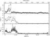 |
Fig. 1 EPIC/PN light curve of 4U 1538−52, binned at 20 s, in the energy ranges 0.3−3 keV (top panel) and 3−11.5 keV (middle panel), and their hardness ratio (bottom panel). |
The XMM-Newton observation of 4U 1538−52 allows us to investigate the pulse profile in detail. To estimate the pulse period, we used the XRONOS version 5.21 timing analysis software package. First of all, we estimated the pulse period with the powspec task; secondly, we searched for the best pulse period with the efsearch task using the χ2 test; and finally, we obtained the folded light curve at the best-fit period P = 526.7 ± 0.2 s. This result is consistent with the RXTE pulse period obtained by Mukherjee et al. (2006), P = 526.849 ± 0.003 s. Figure 2 shows the folded light curves in the two energy intervals 0.3−3 keV (soft) and 3−11.5 keV (hard), together with the folded hardness-ratio. The HR shows two peaks at pulse phases 0.1 and 0.6.
4. Spectral analysis
For spectral analysis we used the XSPEC version 12.5.0 (Arnaud 1996) fitting package, released as a part of XANADU in the HEASoft tools. The EPIC cameras cover the energy range 0.3−11.5 keV. In previous works based on a wider energy range (Tenma, 1.5−35 keV, Makishima et al. 1987; BeppoSAX, 0.1−100 keV, Robba et al. 2001; RXTE, 3−100 keV, Coburn et al. 2002; Rodes 2007; INTEGRAL, 3−100 keV, Rodes-Roca et al. 2009), the X-ray continuum of 4U 1538−52 was described by different absorbed power-law relations, modified by a high-energy cutoff plus a Gaussian emission line at ~6.4 keV, whenever present. Moreover, these models have also been modified by absorption cyclotron resonant scattering features at ~21 keV (Clark et al. 1990; Robba et al. 2001) and at ~47 keV (Rodes-Roca et al. 2009).
Other X-ray continuum models of high-mass X-ray binaries (HMXBs), such as two absorbed power laws or three absorbed power laws, can also describe the observations with ASCA of Vela X−1 (Sako et al. 1999) or with Chandra & XMM-Newton of 4U 1700−37 (Boroson et al. 2003; van der Meer et al. 2005). One power law is used to fit the direct continuum, which originates near the neutron star. Part of this radiation is scattered by the stellar wind of the supergiant star and is fitted by the second power law. Some HMXBs present a soft excess at low energies (0.1−1 keV), which may be modelled as another absorbed power law, blackbody component, or bremsstrahlung component. The physical origin of this component is not understood well, although it is reported for some X-ray binary sources, such as 4U 1700−37 (van der Meer et al. 2005), 4U 1626−67, Cen X-3 or Vela X-1 (Hickox et al. 2004). The BeppoSAX spectrum of 4U 1538−52 showed a soft excess at 0.3−1.0 keV, which was modelled with a blackbody component with a temperature of 0.08 keV (Robba et al. 2001). Moreover, they also obtained a good fit using a bremsstrahlung component with a temperature of 0.10 keV. We used all of these models to fit the XMM-Newton continuum spectrum of 4U 1538−52 and Gaussian functions to describe the emission lines.
4.1. X-ray continuum
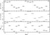 |
Fig. 2 EPIC/PN folded light curves of 4U 1538−52, binned at 20 s, in the energy ranges 0.3−3 keV (top panel), 3−11.5 keV (middle panel), and their hardness ratio (3−11.5)/(0.3−3) (bottom panel). |
When looking for diagnostic emission lines, a proper description of the underlying continuum is critical. Because of its higher count rate we used only the PN spectrum to pin down the parameters of the phase-averaged spectrum and then we combined both PN and MOS pulse phase averaged spectra in order to check our results. We fitted the 0.3−11.5 keV energy spectrum using three absorbed power-law components fixing the photon index parameter to the same value for each power-law component, but with different normalization and column density NH. We modelled the hard X-ray continuum (3−11.5 keV) using two power laws, each of them modified by different absorbing columns (Morrison & McCammon 1983). We obtained adequate fits using the same photon index  for both components, which describe the X-ray continuum radiation from the neutron star: a direct emission from the compact object, absorbed through the surrounding stellar wind, and scattered radiation produced by Thomson scattering by electrons in the extended stellar wind of the supergiant star. Taking the hydrogen columns listed in Table 2 into account, the hard component is assumed to originate in the near surroundings of the neutron star and is highly absorbed by optically thick matter in the line of sight (NH ~ 6.0 × 1023 cm-2), and the scattered component is produced by optically thin plasma (NH ~ 1.2 × 1023 cm-2). Other HMXBs with spectra that can be described by these components are Cen X-3 (Nagase et al. 1992; Ebisawa et al. 1996) and 4U 1700−37 (van der Meer et al. 2005). These systems also showed a hard component that is highly absorbed even during the eclipse.
We used the third absorbed power law because a soft excess at 0.3−1.0 keV is detected in the PN spectrum. We fixed the photon index to that of the other power laws, thereby obtaining a significant improvement ( , with an F-test of 4.2 × 10-131). Figure 3 shows the three different absorbed power-law continuum components and their residuals in units of σ. The spectrum clearly shows several emission lines at 6.4 keV, 2.4 keV, 1.9 keV, and 1.3 keV, and an absorption feature at 2.1 keV. The flux ratios are usually above 30%. We are sure that the low-energy residuals are not due to incomplete calibration. The cross-calibration XMM-Newton database consists of ~150 observations of different sources, optimally reduced, and fit with spectral models defined on a source-by-source basis1. As a result, deviations for PN and MOS flux ratios above 10% are consistent with the presence of emission or absorption lines.
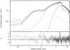 |
Fig. 3 EPIC/PN spectrum of 4U 1538−52 and X-ray continuum model. The dashed line represents the direct component, the dash-dot-dot-dot the scattered component, and the dotted line the soft component (top panel). The lower panel shows the residuals between the spectrum and the model. |
We also used other components to investigate the physical origin of this soft excess, such as a bremsstrahlung or blackbody component. These model components need to be modified by an absorption column too. Although a bremsstrahlung component improves the fit significantly ( , F-test of 4.0 × 10-131), its inferred temperature is too high (196.9 keV) and could not be constrained within the XMM band pass, suggesting that the soft excess has another physical origin. In Table 2 we report the model parameters of the X-ray continuum spectrum for the PN camera. All uncertainties refer to a single parameter at the 90% (Δχ2 = 2.71) confidence limit2.
When we used a blackbody component we also obtained a similar improvement in the fit (, F-test of 1.6 × 10-129). The blackbody has a temperature of  keV. We calculated the luminosity of the source of the blackbody component over the 0.3−11.5 keV energy band, assuming a distance to the source of 5.5 kpc (Becker et al. 1977) and isotropic emission to be 5.4 × 1033 erg s-1. Since the surface luminosity of a blackbody only depends on its temperature, it is possible to calculate the size of the emitting region:
 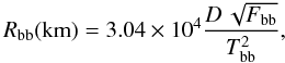 (1)where D is the distance to the source in kpc, Fbb the unabsorbed flux over the 0.3−11.5 keV energy band in erg s-1 cm-2, Tbb the temperature in keV, and Rbb is the radius of the emitting region. From Eq. (1), we found a radius of the emitting surface of 0.24 km. If we assume thermal emission from the neutron star polar cap, this radius may be consistent with the expected size. However, we estimated the radius of the accreting polar cap using the equation (Hickox et al. 2004):
 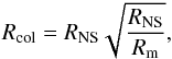 (2)where Rm is the magnetospheric radius and RNS the neutron star radius. The magnetospheric radius may be estimated from the magnetic dipole moment and mass accretion rate (Elsner & Lamb 1977; Audley et al. 1996):
 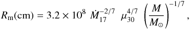 (3)where μ30 is the magnetic dipole moment of the neutron star in units of 1030 G cm3 and Ṁ17 is the mass accretion rate in units of 1017 g s-1. With M = 1.3 M⊙ (Reynolds et al. 1992), Ṁ17 = 883 g s-1 (Clark et al. 1994; Rodes 2007; Rodes et al. 2008), and μ30 = 1.8 G cm3 (Rodes 2007), the Eq. (3) yields the value Rm ~ 6.2 × 107 cm. Assuming RNS ~ 106 cm, we obtained Rcol ~ 1.27 km, five times our estimated blackbody emitting radius. Although this result suggests that the soft excess is not formed by blackbody emission, taking the associated errors in the parameters into account, we cannot exclude blackbody emission as the origin of the soft excess.
We also tried to fit this soft excess by adding 2 to the photon index of the soft component compared to the index of the hard component, i.e. scattering by dust grains at large distances from the source (Robba et al. 2001; van der Meer et al. 2005). We obtained a good description of the spectrum ( , F-test of 11 × 10-116), but a significantly worse fit than the previous components ().
Finally, we modelled the soft X-ray continuum component with only a blend of Gaussians (Boroson et al. 2003; van der Meer et al. 2005) and refitted the data. We could not obtain a good description below 0.6 keV, though. Therefore, although the model composed of three power-law components also does not fit the data well below 0.6 keV, it was the best model obtained, so we used it for our analysis.
Afterwards we combined EPIC/PN and EPIC/MOS spectra and applied the same models to them to obtain similar results. The spectra of all three EPIC instruments were fitted simultaneously, including a factor to allow for the adjustment of efficiencies between different instruments. We fixed the continuum parameters, as described in Table 2, and looked for the emission features (see Sect. 4.2).
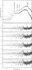 |
Fig. 4 Fluorescence emission lines modelling of the phase-averaged spectra PN & MOS of 4U 1538−52. Top panel: spectra and best-fit model (three absorbed power laws and four emission lines) obtained with EPIC/PN and EPIC/MOS. Bottom panels show the residuals in units of σ for models taking different numbers of emission lines into account (MOS-1 black filled square and MOS-2 grey cross). Second panel: without emission lines. Third panel: fluorescence iron emission line at ~6.4 keV. Fourth panel: fluorescence iron emission line plus a recombination line at ~2.42 keV. Fifth panel: fluorescence iron emission line plus two recombination lines at ~2.42 keV and ~1.90 keV. Bottom panel: fluorescence iron emission line plus three recombination lines at ~2.42 keV, ~1.90 keV and ~1.34 keV. |
4.2. Emission lines
The X-ray eclipse spectra of some HMXBs show many emission lines and radiative recombination continua (e.g. Vela X-1, Sako et al. 1999; Cen X-3 Ebisawa et al. 1996; 4U 1700−37 van der Meer et al. 2005). These data are included in Fig. 4, together with the best-fit model, three absorbed power laws plus emission lines, and residuals of the fit as the difference between observed flux and model flux divided by the uncertainty of the observed flux, i.e. in units of σ. As we can see in Fig. 4, the PN spectrum of 4U 1538−52 shows emission lines below 3 keV and between 6 and 7 keV. We fitted these lines as Gaussian profiles (see Table 3 for parameter values). Because the energy resolution of the EPIC cameras is not high enough to resolve all lines (FWHM 80−100 eV in the energy range 1−3 keV), many of them could be blended (e.g., 1.75 keV Si Kα, Al xiii Lyα, and 1.85 keV Si xiii Heα). Using the list of emission lines in van der Meer et al. (2005), we could identify suitable candidates among fluorescence emission lines from near-neutral species and discrete recombination lines from He- and H-like species (see also Drake 1988; Hojnacki et al. 2007).
Figure 4 clearly shows the presence of the Fe Kα line at ~6.4 keV, but a second broad emission line around 6.65 keV or an absorption edge at ~7.2 keV associated with low-ionization iron is an unresolved issue within the deviation for PN and MOS ratios.
We started by modelling the fluorescence iron line (see Fig. 4) that was also detected by several other satellite observatories, such as Tenma, BeppoSAX, or RXTE. Starting with the 3PL continuum model, after including the emission line at E ~ 6.4 keV, the  improves from 1.16 for 2242 degrees of freedom (d.o.f.) to 1.08, for 2239 d.o.f. (F-test of 9.2 × 10⁻³⁵). Although residuals improve significantly above 3 keV (see Fig. 4 third panel), other emission features can be seen at ~2.4, ~ 1.9 keV, and ~1.3 keV. Including an emission line at ~2.4 keV improves the fit, further resulting in a of 1.07 for 2236 d.o.f. (F-test of 9.5 × 10⁻⁶, see Fig. 4 fourth panel). Adding another one at ~1.9 keV, we obtained a of 1.06 for 2233 d.o.f. (F-test of 2.6 × 10⁻⁶, see Fig. 4 fifth panel). Finally, the last emission line at ~1.3 keV marginally improves the fit, leading to = 1.05 for 2230 d.o.f. (F-test of 0.4, see Fig. 4 bottom panel).
Using the combined spectra, we did not obtain an improvement in the fit quality ( , compared to obtained using only the PN spectrum). Nevertheless, as is clear from Fig. 4, the emission lines are seen in the raw data of the three cameras. In Table 3 we show the best-fit parameters for the emission lines we detected in Fig. 4, where the top spectrum in the top panel is from PN and the bottom spectra in the top panel are from MOS-1 and MOS-2, respectively.
The F-test is known to be problematic when used to test the significance of an additional spectral feature (see Protassov & van Dik 2002), even if systematic uncertainties are not an issue. However, the low-false alarm probabilities may make the detection of the line stable against even crude mistakes in computing significance (Kreykenbohm 2004). Therefore, considering these caveats, we can conclude that the fluorescence emission lines are detected with high significance in the spectrum of this source and that none of these features is the result of poor calibration.
However, these models do not deal with the strong feature at ~2.1 keV. We added a Gaussian absorption profile at this energy and found an improvement in the fit, but the high optical depth and its unconstrained value prevent us from accepting it. We checked the possibility that this feature could be a gain effect by changing the gain and offset values by up to ±3% and ±0.05 keV, respectively. The line profile expressed as the ratio of a spectral data to a best-fit model was always around 70%, suggesting that it is not a gain effect and that the absorption feature could be real. Moreover, although the feature is less pronounced in a spectrum extracted only using single pixel events, the EPIC/PN calibration team have confirmed (M. Guainazzi, priv. comm.) the reality of the absorption feature at 2.1 keV.
4.3. Pulse-phase resolved spectra
The hardness ratio shown in Fig. 2 demonstrates variation in the spectrum with respect to the spin phase of the neutron star. We divided the pulse into ten phase intervals of equal length in order to investigate the X-ray spectrum as a function of pulse phase. We produced energy spectra corresponding to each of these phase intervals, which were fitted by the same X-ray underlying model used to fit the pulse-phase averaged spectrum, i.e., three absorption power laws plus an iron emission line. The resulting fit parameters are reported in Table 4.
Results of the fit of the pulse-phase resolved spectra in the energy range 0.3−11.5 keV.
We did not find any statistically significant residuals in the energy range between 1 and 3 keV; therefore, no low-energy emission lines are required to fit these spectra, although this could be because of the lower statistics of the phase resolved spectra with respect to the phase-averaged spectrum. The energy of the iron emission line is compatible with being unchanged along the pulse profile, although the variations in the depth, width, and equivalent width could be due to the presence of other unresolved emission lines. The BeppoSAX spectrum showed similar results with the pulse phase of the iron emission line parameters using four phase intervals (Robba et al. 2001). In other pulse-phase spectroscopy analysis either the iron emission line was not present significantly (EXOSAT; Robba et al. 1992) or was also unchanged when the pulse phase profile was divided into two phase intervals (Tenma; Makishima et al. 1987). The variation in the different column absorption parameters are significant along the pulse profile, but again these do not show a clear relationship to the other parameters.
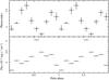 |
Fig. 5 Photon index (top panel) and the corresponding unabsorbed flux in the 0.3−11.5 energy band (10-10 erg s-1 cm-2, lower panel) versus the corresponding phase interval. |
The photon index presents a clear modulation with the pulse phase showing two maximum values at phases 0.35 and 0.85 and one minimum value at phase 0.65. In Fig. 5 we plot the photon index (top panel) versus the corresponding phase interval together with the corresponding unabsorbed flux in the 0.3−11.5 keV energy band (lower panel). As can be seen from this figure, the phase of maximum unabsorbed flux is close to the phase of minimum photon index, but there is not a one-to-one correspondence between these two parameters. The unabsorbed flux presents two flat regions in the phase intervals 0.15−0.35 and 0.65−0.85 and increasing or decreasing flux in the other interval phases. It peaks at phase 0.55 and is near the minimum in the photon index. The result obtained from BeppoSAX shows a clear anticorrelation between the photon index and the flux, with the spectrum flatter in correspondence with higher flux levels (Robba et al. 2001). Moreover, this behaviour of the photon index from BeppoSAX is similar to previous results from EXOSAT (Robba et al. 1992) and Ginga (Clark et al. 1990).
4.4. Detecting emission lines in the eclipse spectrum
As shown in Sect. 3, the eclipse of the X-ray source is clearly visible in the last 55 ks of the XMM-Newton observation (see Fig. 1). Therefore, we analysed the phase-averaged spectrum out of eclipse and in eclipse. The X-ray continuum spectrum out of the eclipse could be described by the models used in this work. While the parameters of the fluorescent iron emission line at 6.4 keV were consistent with those of the whole observation, we did not find any evidence of the other emission lines. Nevertheless, Fig. 1 suggests the presence of a variability out of the eclipse since the HR changes with time. Therefore, we divided the data out of the eclipse into two temporal intervals, 0−10 ks and 10−20 ks, taking the HR variability into account. We could describe these spectra with the same X-ray continuum, i.e. three absorbed power-law components and a fluorescence iron emission line. No statistically significant residuals were observed in the energy range between 1 and 3 keV, and therefore no more emission lines are required to fit these spectra. The photon index and the iron emission line were compatible within the associated errors, but the photoelectric absorption were significantly different.
The continuum spectrum in eclipse was described by two absorbed power laws because the direct component should not be seen in the eclipse. In Fig. 6 we show the eclipse spectra (top panel) and the residuals to the two absorbed power-law continuum model from PN and MOS cameras simultaneously (second panel). Although the fit quality is very good, the high value deduced for the absorption column is at odds with the interpretation of this power law as the scattered component. In fact, the values are more consistent with those of the hard component. However, any other combination we tried resulted in significantly worse fits. Whatever the interpretation might be, this component seems to be the dominant one both in and out of eclipse.
4U 1538−52 shows some emission lines in the eclipse, when the X-ray continuum emission is at a minimum. Evident are the presence of the Fe Kα line at 6.4 keV, an absorption edge around 7.1 keV, and emission lines between 1 and 3 keV. We fixed the two absorbed power-law components and added Gaussian profiles to fit these emission lines. Table 5 lists the parameters of the continuum model we used to fit the spectra.
Figure 6 shows the spectra and the residuals with respect to X-ray continuum model in the whole energy range 0.3−11.5 keV using the PN and MOS cameras. We note that in the 6.4−7.2 keV energy band, some iron emission lines are present in the residuals. As shown using high-resolution Chandra/HETG data (Brandt & Schulz 2000; D’Aí et al. 2007), the Fe complex can be clearly resolved into the near neutral Fe Kα line plus hot lines from highly ionized species of Fe XXV and Fe XXVI. Therefore, we used Gaussian lines to fit these residuals. In the bottom panels of Fig. 6 we show the ratio before and after adding the emission lines described in this section. In Table 6, we report the parameters of the iron emission lines. The parameters of the Gaussian emission lines are energy, σ, and EW, indicating the centroid, the width, and the equivalent width, respectively.
The EW of the neutral iron Kα line is noticeably larger in eclipse (262 eV) than out of eclipse (~30 eV). Rodes et al. (2006) find that the EW was larger when the source flux was low by using an RXTE observation that covers nearly a complete orbital period. The measured line energy is consistent with an ionization stage up to Fe XVII, and this requires that the ionization parameter ξ is less than several hundred erg cm s-1 (Kallman & McCray 1982; Ebisawa et al. 1996).
On the other hand, the simultaneous presence of the Fe XXV line in the spectrum implies an ionization parameter for the photoionized plasma of ξ ~ 103.2 erg cm s-1 (Ebisawa et al. 1996). The broad range of the ionization parameter suggests either that the emitting material is present over a wide range of distances from the neutron star or has a wide range of densities.
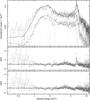 |
Fig. 6 Iron emission lines and recombination emission lines of He- and H-like species in the eclipse spectrum of 4U 1538−52. Top panel: spectra and best-fit model (two absorbed power laws and six emission lines) in the 0.3−11.5 keV energy range obtained with PN (top) and MOS (light grey filled squared and dark grey cross) cameras. Bottom panels show the residuals. Second panel: without emission lines. Third panel: with iron and recombination of He- and H-like emission lines for the combined spectra. |
Figure 6 also shows the residuals with respect to a continuum model consisting of two power laws in the 1.0−3.0 keV energy range, each with a different absorbing column. Discrete recombination lines from He- and H-like species are present in the MOS and PN spectra of 4U 1538−52. The energy resolution of the instruments is not sufficient to resolve the lines clearly (Drake 1988; Hojnacki et al. 2007). Therefore, our identification could be a blend of other emission lines. We also fit these emission lines as Gaussians and list them in Table 6.
5. Summary and discussion
We presented the spectral analysis of the HMXB 4U 1538−52 using an XMM-Newton observation. The X-ray continuum is well fitted by three absorbed power laws with a photon index ~1.13, describing the hard, scattered, and soft excess. The inferred unabsorbed flux is ~2.1 × 10⁻¹⁰ erg s-1 cm-2 in the 0.3−11.5 keV energy band, corresponding to a luminosity of ~7.5 × 1035 erg s-1, assuming an isotropic emission and a distance to the source of 5.5 kpc (Becker et al. 1977). The flux found by RXTE in the 3−11.5 keV energy band and an orbital phase of 0.85 was 1.3 × 10⁻¹⁰ erg s-1 cm-2. Using the spectrum obtained by XMM-Newton over the same range of phases, the flux we obtained in this work was two times lower, 6.3 × 10⁻¹¹ erg s-1 cm-2.
The soft excess is present in the spectrum and can be modelled with different absorbed components. We simply modelled the soft emission with an absorbed power-law component, although Fig. 4 still showed spectral residuals at the lowest energies. Our results show that a blackbody component could also be the physical origin of this soft excess, when taking the associated errors into account. The soft excess in other HMXBs has been explained by a blend of Gaussian emission lines alone (Boroson et al. 2003). We also tried to fit the soft emission using Gaussian profiles, but we did not obtain a significant improvement in the fit because of the low level of counts below 0.6 keV.
We detected an iron Kα line at ~6.41 keV, with an EW of ~50 eV. The BeppoSAX observation of this system obtained an EW of 57 eV in the same orbital phase range 0.75−1.00 (Robba et al. 2001) and showed an increase in the post-egress phase to 85 eV. The phase-averaged spectrum obtained by RXTE reported an EW of 62 eV (Coburn et al. 2002). In addition this iron line is detected in all orbital phases (Robba et al. 2001; Rodes 2007), therefore the Kα iron line is not only produced by fluorescence from less ionized iron near the neutron star’s surface but also a fraction of the observed line flux must originate from more extended regions. We also detected a number of emission lines that we interpret as recombination lines from highly ionized species. Since these lines are detected in eclipse, they must be produced in an extended halo. Likewise, we have found an absorption feature at 2.1 keV. Whether it is produced by physical properties of the source or comes from calibration effects is still an open issue.
We compared the phase-average spectrum to the eclipse spectrum. In the phase-average spectrum, we found no evidence of any other iron line apart from the one at 6.4 keV, and the absorption edge at ~7.1 keV was described by the X-ray absorption model well. The 6.4−7.2 keV energy band showed a complex structure, but we did not find any proper model to describe it or detect other iron features significantly. We also detected discrete recombination lines in both EPIC/PN and EPIC/MOS spectra. The emission lines reported in Sect. 4.2 can be identified with He- and H-like ions. Although we could identify some of them, the energy resolution of the EPIC instruments is such that the lines could be blended.
However, in the eclipse spectrum, we detected the fluorescence iron line at 6.4 keV and one more iron emission line at 6.6 keV. The discrete recombination lines we detected are listed in Table 6. The presence of these lines in an eclipse spectrum implies that the formation region extends beyond the size of the B supergiant. Moreover, the ionization state was estimated to range from 102.1 to 103.2 erg cm s-1, due to the simultaneous detection of elements with both low and high ionization levels. This broad range of ξ also suggests that the emitting material is either present over a wide range of distances from the compact object or has a wide range of densities.
The pulse phase-resolved spectroscopy showed significant variability in the photon index and the unabsorbed flux, but there was no clear correlation or anticorrelation between them. Significant variations with the pulse phase were also observed in the different column absorption values, but again it did not show a clear relationship to the other parameters.
Future observations with high spectral resolution instruments will be needed to unambiguously resolve any possible blended lines found in this study allowing the full use of their diagnostic capability.
Acknowledgments
Part of this work was supported by the Spanish Ministry of Education and Science Primera ciencia con el GTC: La astronomía española en vanguardia de la astronomía europea CSD200670 and Multiplicidad y evolución de estrellas masivas project number AYA200806166C0303 and partially supported by AYA2010-15431. This research made use of data obtained through the XMM-Newton Science Archive (XSA), provided by European Space Agency (ESA). We are grateful to the anonymous referee for useful and detailed comments. We would like to thank the XMM helpdesk, particularly Matteo Guainazzi, for invaluable assistance in determining the systematic uncertainties in the PN data. K.L.P. and J.P.O. acknowledge support from STFC. J.J.R.R. acknowledges the support by the Spanish Ministerio de Educación y Ciencia under grant PR2009-0455.
References
- Arnaud, K. A. 1996, in Astronomical Data Analysis Software and Systems V, ed. J. H. Jacoby, & J. Barnes, San Francisco, ASP Conf. Ser., 101, 17 [Google Scholar]
- Audley, M. D., Kelley, R. L., Boldt, E. A., et al. 1996, ApJ, 457, 397 [NASA ADS] [CrossRef] [Google Scholar]
- Becker, R. H., Swank, J. H., Boldt, E. A., et al. 1977, ApJ, 216, L11 [NASA ADS] [CrossRef] [Google Scholar]
- Brandt, W. N., & Schulz, N. S. 2000, ApJ, 544, L123 [NASA ADS] [CrossRef] [Google Scholar]
- Boroson, B., Vrtilek, S. D., Kallman, T., et al. 2003, ApJ, 592, 516 [NASA ADS] [CrossRef] [Google Scholar]
- Clark, G. W. 2000, ApJ, 542, L131 [NASA ADS] [CrossRef] [Google Scholar]
- Clark, G. W., Woo, J. W., Nagase, F., et al. 1990, ApJ, 353, 274 [NASA ADS] [CrossRef] [Google Scholar]
- Clark, G. W., Woo, J. W., & Nagase, F. 1994, ApJ, 422, 336 [NASA ADS] [CrossRef] [Google Scholar]
- Coburn, W., Heindl, W. A., Rothschild, R. E., et al. 2002, ApJ, 580, 394 [NASA ADS] [CrossRef] [Google Scholar]
- Corbet, R. H. D., Woo, J. W., & Nagase, F. 1993, A&A, 276, 52 [NASA ADS] [Google Scholar]
- D’Aí, A., Iaria, R., Di Salvo, T., et al. 2007, ApJ, 671, 2006 [NASA ADS] [CrossRef] [Google Scholar]
- Davison, P. J. N., Watson, M. G., & Pye, J. P. 1977, MNRAS, 181, 73P [NASA ADS] [CrossRef] [Google Scholar]
- Drake, G. W. 1988, Canadian J. Phys., 66, 586 [Google Scholar]
- Ebisawa, K., Day, C. S. R., Kallman, T. R., et al. 1996, PASJ, 48, 425 [NASA ADS] [Google Scholar]
- Elsner, R. F., & Lamb, F. K. 1977, ApJ, 215, 897 [NASA ADS] [CrossRef] [Google Scholar]
- Giacconi, R., Gursky, H., Kellog, E., et al. 1974, ApJS, 27, 37 [NASA ADS] [CrossRef] [Google Scholar]
- Harding, A. K., & Daugherty, J. K. 1991, ApJ, 374, 687 [NASA ADS] [CrossRef] [Google Scholar]
- Hatchett, S., & McCray, R. 1977, ApJ, 211, 552 [NASA ADS] [CrossRef] [Google Scholar]
- Hickox, R. C., Narayan, R., & Kallman, T. R. 2004, ApJ, 614, 881 [NASA ADS] [CrossRef] [Google Scholar]
- Hojnacki, S. M., Kastner, J. H., Micela, G., et al. 2007, ApJ, 659, 585 [NASA ADS] [CrossRef] [Google Scholar]
- Iaria, R., Di Salvo, T., Robba, N. R., et al. 2005, ApJ, 634, L161 [NASA ADS] [CrossRef] [Google Scholar]
- Kallman, T. R., & McCray, R. 1982, ApJS, 50, 263 [NASA ADS] [CrossRef] [Google Scholar]
- Kreykenbohm, I. 2004, Ph.D. Thesis, University of Tübingen [Google Scholar]
- Makishima, K., Koyama, K., Hayakawa, S., et al. 1987, ApJ, 314, 619 [NASA ADS] [CrossRef] [Google Scholar]
- Morrison, R., & McCammon, D. 1983, ApJ, 270, 119 [NASA ADS] [CrossRef] [Google Scholar]
- Mukherjee, U., Raichur, H., Paul, B., et al. 2006, JAA, 27, 411 [Google Scholar]
- Nagase, F., Corbet, R. H. D., Day, C. S. R., et al. 1992, ApJ, 396, 147 [NASA ADS] [CrossRef] [Google Scholar]
- Protassov, R., & van Dik, D. A. 2002, ApJ, 571, 545 [NASA ADS] [CrossRef] [Google Scholar]
- Reynolds, A. P., Bell, S. A., & Hilditch, R. W. 1992, MNRAS, 256, 631 [NASA ADS] [Google Scholar]
- Robba, N. R., Cusumano, G., Orlandini, M., et al. 1992, ApJ, 401, 685 [NASA ADS] [CrossRef] [Google Scholar]
- Robba, N. R., Burderi, L., Di Salvo, T., et al. 2001, ApJ, 526, 950 [NASA ADS] [CrossRef] [Google Scholar]
- Rodes, J. J. 2007, Ph.D. Thesis, University of Alicante, http://hdl.handle.net/10045/13227 [Google Scholar]
- Rodes, J. J., Torrejón, J. M., & Bernabéu, G. 2006, Proceedings of the The X-ray Universe 2005, 26−30 September 2005, El Escorial, Madrid, Spain, ed. A. Wilson (Noordwijk: ESA Publications Division), ESA SP-604, 1, 287 [Google Scholar]
- Rodes, J. J., Torrejón, J. M., & Bernabéu, G. 2008, The X-ray Universe 2008, 27−30 May 2008, Granada, Spain, http://xmm.esac.esa.int/external/xmm_science/workshops/2008symposium/#topicB [Google Scholar]
- Rodes-Roca, J. J., Torrejón, J. M., Kreykenbohm, I., et al. 2009, A&A, 508, 395 [NASA ADS] [CrossRef] [EDP Sciences] [Google Scholar]
- Sako, M., Liedahl, D. A., Kahn, S. M., et al. 1999, ApJ, 525, 921 [NASA ADS] [CrossRef] [Google Scholar]
- Strüder, L., Briel, U., Dennerl, K., et al. 2001, A&A, 365, L18 [NASA ADS] [CrossRef] [EDP Sciences] [Google Scholar]
- Turner, M. J. L., Abbey, A., Arnaud, M., et al. 2001, A&A, 365, L27 [NASA ADS] [CrossRef] [EDP Sciences] [Google Scholar]
- van der Meer, A., Kaper, L., Di Salvo, T., et al. 2005, A&A, 432, 999 [NASA ADS] [CrossRef] [EDP Sciences] [Google Scholar]
- van Loon, J. Th., Kaper, L., & Hammerschlag-Hensberge, G. 2001, A&A, 375, 498 [NASA ADS] [CrossRef] [EDP Sciences] [Google Scholar]
- White, N. E., Swank, J. H., & Holt, S. S. 1983, ApJ, 270, 711 [NASA ADS] [CrossRef] [Google Scholar]
All Tables
Results of the fit of the pulse-phase resolved spectra in the energy range 0.3−11.5 keV.
All Figures
|
Fig. 1 EPIC/PN light curve of 4U 1538−52, binned at 20 s, in the energy ranges 0.3−3 keV (top panel) and 3−11.5 keV (middle panel), and their hardness ratio (bottom panel). |
| In the text | |
|
Fig. 2 EPIC/PN folded light curves of 4U 1538−52, binned at 20 s, in the energy ranges 0.3−3 keV (top panel), 3−11.5 keV (middle panel), and their hardness ratio (3−11.5)/(0.3−3) (bottom panel). |
| In the text | |
|
Fig. 3 EPIC/PN spectrum of 4U 1538−52 and X-ray continuum model. The dashed line represents the direct component, the dash-dot-dot-dot the scattered component, and the dotted line the soft component (top panel). The lower panel shows the residuals between the spectrum and the model. |
| In the text | |
|
Fig. 4 Fluorescence emission lines modelling of the phase-averaged spectra PN & MOS of 4U 1538−52. Top panel: spectra and best-fit model (three absorbed power laws and four emission lines) obtained with EPIC/PN and EPIC/MOS. Bottom panels show the residuals in units of σ for models taking different numbers of emission lines into account (MOS-1 black filled square and MOS-2 grey cross). Second panel: without emission lines. Third panel: fluorescence iron emission line at ~6.4 keV. Fourth panel: fluorescence iron emission line plus a recombination line at ~2.42 keV. Fifth panel: fluorescence iron emission line plus two recombination lines at ~2.42 keV and ~1.90 keV. Bottom panel: fluorescence iron emission line plus three recombination lines at ~2.42 keV, ~1.90 keV and ~1.34 keV. |
| In the text | |
|
Fig. 5 Photon index (top panel) and the corresponding unabsorbed flux in the 0.3−11.5 energy band (10-10 erg s-1 cm-2, lower panel) versus the corresponding phase interval. |
| In the text | |
|
Fig. 6 Iron emission lines and recombination emission lines of He- and H-like species in the eclipse spectrum of 4U 1538−52. Top panel: spectra and best-fit model (two absorbed power laws and six emission lines) in the 0.3−11.5 keV energy range obtained with PN (top) and MOS (light grey filled squared and dark grey cross) cameras. Bottom panels show the residuals. Second panel: without emission lines. Third panel: with iron and recombination of He- and H-like emission lines for the combined spectra. |
| In the text | |
Current usage metrics show cumulative count of Article Views (full-text article views including HTML views, PDF and ePub downloads, according to the available data) and Abstracts Views on Vision4Press platform.
Data correspond to usage on the plateform after 2015. The current usage metrics is available 48-96 hours after online publication and is updated daily on week days.
Initial download of the metrics may take a while.