| Issue |
A&A
Volume 525, January 2011
|
|
|---|---|---|
| Article Number | A112 | |
| Number of page(s) | 7 | |
| Section | The Sun | |
| DOI | https://doi.org/10.1051/0004-6361/201015600 | |
| Published online | 06 December 2010 | |
Flare quasi-periodic pulsations with growing periodicity
1
Nobeyama Solar Radio Observatory / NAOJ,
Nagano
384-1305,
Japan
e-mail: This email address is being protected from spambots. You need JavaScript enabled to view it.
; This email address is being protected from spambots. You need JavaScript enabled to view it.
2
Radiophysical Research Institute (NIRFI),
Nizhny Novgorod
603950,
Russia
Received:
17
August
2010
Accepted:
27
October
2010
Abstract
We conducted a wavelet analysis of the flare intensity variations for the long duration flare on 2005 August 22 observed with the Nobeyama Radioheliograph at frequencies 17 and 34 GHz and with the Ramaty High Energy Solar Spectroscopic Imager at 25–50 keV. We found that the signals contain a well-pronounced periodicity in which the oscillation period grows from 2.5 to 5 min. An analysis of the loop length and plasma temperature evolution during the flare allowed us to interpret the quasi-periodic pulsations in terms of the second standing harmonics of the slow magnetoacoustic mode. This mode can be generated by the initial impulsive energy release and work as a trigger for the repeated energy releases.
Key words: magnetohydrodynamics (MHD) / waves / Sun: flares / Sun: oscillations / Sun: radio radiation / Sun: X-rays, gamma rays
© ESO, 2010
1. Introduction
Quasi-periodic pulsation (QPP) with periods from tens of seconds to tens of minutes are often observed in solar flare light curves in radio and X-ray bands (see Nakariakov & Melnikov 2009, for a review). These long period coronal oscillations are believed to be associated with magnetohydrodynamic (MHD) waves or/and to be generated by magnetic reconnection. Therefore, these oscillations are of fundamental importance, because they can provide information about mechanisms responsible for the energy release, its triggering, and processes operating in them.
Possible MHD modes for the interpretation of these long QPP are kink mode (Zaitsev & Stepanov 1989) or slow acoustic mode (Nakariakov et al. 2000). These MHD oscillation modes have now been detected with imaging observations. The most reliable identifications were made in coronal structures without flares. Longitudinal slow magnetoacoustic modes are the most frequently observed in solar coronal structures. This mode, producing noticeable perturbations of the loop density and generating field-aligned flows, can be either propagating or standing. A propagating acoustic wave has been identified as periodic EUV emission disturbances along polar plumes (DeForest & Gurment 1998; Ofman et al. 1999) and long loops (Berghmans & Clette 1999; De Moortel 2006), with typical periods ranging from 2 to 15 min. Hinode/EIS observations revealed 5 min quasiperiodic oscillations in a coronal loop with an in-phase relation between Doppler shift and intensity (Wang et al. 2009a) and propagating disturbances along a fan-like coronal structure with periods of 12 and 25 min (Wang et al. 2009b). Both observations indicated upward propagating slow magnetoacoustic waves. A standing slow magnetoacoustic mode, which may arise only in a coronal loop with the ends embedded in a high-density chromosphere-photosphere, was detected as the Doppler shift and EUV emission intensity variations (Wang et al. 2002, 2003). The oscillation periods were found to be in the range of 7 to 30 min, and the oscillation amplitude is typically about 10–20%, in some cases reaching 50% of the background.
Quasi-periodic modulations of the microwave emission from solar flares with periods of 3, 5, and 10 min observed at 37 GHz were interpreted in terms of the LCR-circuit model (Zaitsev & Kislyakov 2006). According to their model, 5 min photospheric oscillations (p-modes) modulate a convection velocity and electric current in a coronal arch. When the electric current oscillations coincide with resonant frequencies of acoustic oscillations in the arch, the last ones are excited. The 5-min flaring variations of dm-radio fluxes (Mészárosová et al. 2006) were interpreted as variations of the magnetic field that modulate the flare reconnection process including particle acceleration.
Flaring microwave QPP with a period of 3 min observed over sunspots were discovered with the Nobeyama Radioheliograph (Sych et al. 2009). They are proposed to be triggered by 3-min slow magnetoacoustic waves leaking from sunspots.
The other potential mechanism for the generation of this mode is an impulsive energy release that results in a rapid local increase in the pressure gradient. It was shown by Nakariakov et al. (2004) that if the energy deposition is located near the loop top, the preferentially excited mode is the second harmonics of slow acoustic wave. With help of numerical modeling the authors demonstrated that this mode can be a natural response of a coronal loop to an initial impulsive deposition of energy in the flare. Moreover, Tsiklauri et al. (2004) showed that single footpoint heat positioning still produces second spatial harmonics, though it is more complex than the apex heating. Therefore, the second standing acoustic mode may be responsible for quasi-periodic pulsation with periods in the range 10–300 s, which are often observed in flare light curves in radio and X-ray bands.
Our motivation was to find an observational confirmation of this idea using the imaging observations of Nobeyama Radioheliograph (Nakajima et al. 1994). One of the possibilities of an acoustic wave detection in the radio band is through the modulation of the gyrosynchrotron emission via perturbation of the efficiency in the Razin suppression (Nakariakov & Melnikov 2006). Apart from the emission modulation, the wave itself can play a role of periodic triggering of the energy releases. It was proposed that a compressible wave can periodically trigger magnetic reconnection either by the variation of the plasma density in the vicinity of the reconnection site (Chen & Priest 2006) or by a sharp increase of the electric current density in current sheets (Nakariakov et al. 2006). Both processes can provoke a generation of anomalous resistivity. In this situation a repetitive burst with a periodicity equal to the period of the second standing acoustic mode will be observed. This period is determined approximately by the ratio of the loop length to the average sound speed (Nakariakov et al. 2004).
The high spatial (5′′ at 34 GHz and 10′′ at 17 GHz) and temporal (up to 0.1 s) resolution of Nobeyama Radioheliograph (NoRH) allows us to obtain the information about the longitudinal and transverse sizes of the microwave flaring loop and their dynamics. An evolution of plasma temperature can be obtained from GOES X-ray observations. Therefore, we can estimate the mode period and its evolution and compare it with observed QPP dynamics. With NoRH we can also study the spatial structure of the oscillations in different parts of the flaring loop, which is important for the mode identification too.
In this paper we use this possibility to examine quasi-periodic pulsations during the flare of 2005 August 22 observed in microwaves and hard X-rays.
2. Observations
The intense solar flare occurred 2005 August 22 at 00:54 UT with heliographic coordinates S12°, W49° and was connected with the active region (AR) NOAA 10798. GOES fluxes in channels 1−8 Å (thick line) and 0.5−4 Å (thin line) are shown in Fig. 1a. The flare was of the M2.6 class on the GOES scale and was related to the long duration events. The corresponding microwave burst was observed by the Nobeyama Radioheliograph at two frequencies, 17 and 34 GHz, and by Nobeyama Radiopolarimeter (NoRP). Figure 1b shows the NoRP time profile at 2 GHz and the NoRH time profiles of the total fluxes integrated over the partial images, the size of 313′′ × 313′′, which includes the whole AR. They display multiple emission peaks at all frequencies.
The Ramaty High Energy Solar Spectroscopic Imager (RHESSI) was in the shadow of the Earth until 01:02 UT, therefore, observations of the X-ray burst started only after the main peak on the NoRH/NoRP time profiles. The RHESSI count rate in the channel 25–50 keV is shown in Fig. 1c. The time profiles of hard X-rays clearly display damped quasi-periodical pulsations.
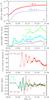 |
Fig. 1 Light curves of the flare. a) Soft X-ray in the GOES 1 − 8 Å (thick line) and 0.5 − 4 Å (thin line) channels; b) NoRP flux at 2 GHz (green) and NoRH fluxes integrated over the AR at 17 GHz (blue), and 34 GHz (black); c) hard X-ray count rate measured in RHESSI 25–50 keV channel; d) modulation depth of emission at frequencies 2 GHz (green), 17 GHz (blue), 34 GHz (black) and energy 25–50 keV (red). |
In Fig. 1d we show the modulation depth of emissions observed by three different instruments, NoRP (2 GHz), NoRH (17, 34 GHz), and RHESSI (25–50 keV). The modulation depth of the signal is calculated as 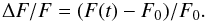 (1)The slowly varying mean signal F0 is obtained by 200 s smoothing of the signal. Radio emission at all three frequencies shows pulsations with an inphase behavior and a modulation depth of up to 20%. The hard X-ray emission exhibits a higher modulation depth of up to 30%. Li & Gan (2008) found for this event using RHESSI data that the modulation depth increases with the energy up to 90%. Microwave pulsations at 17 GHz (34 GHz) delay 36 s (52 s) against HXR pulsations, they are highly correlated, correlation coefficient R = 0.7 (R = 0.6). It is well known that microwave emission is produced by gyrosynchrotron radiation of nonthermal electrons with energies in excess of 100 keV trapped in the flare loop. Their average lifetime is longer than lower energy (tens of keV) electrons generating hard X-rays by bremsstrahlung.
Figure 2 shows images of the flare loop at 17 GHz (Stokes I) at different moments of the burst. We used Fujiki synthesis programs to obtain the partial Sun images with a field of view of 128 × 128 pixels and pixel size 2.45 arcsec. Contours at levels 0.1, 0.3, 0.5, 0.7, 0.9 of maximum brightness temperature  are shown. On Fig. 2a the level 0.05 of is also presented. Dot-dashed lines show visible flaring loop axes. They were drawn using a spline approximation through the brightest points along the loop between two footpoints on levels 0.1 of . This level corresponds on average to the centers of HXR-sources and consequently to the level of Sun’s chromosphere where the loop ends are anchored.
 |
Fig. 2 NoRH images of the flare source at 17 GHz, I at different moments in time. Contours correspond to 0.1, 0.3, 0.5, 0.7, 0.9 levels of maximum |

The entire loop structure was well seen during all the burst, but its length and orientation changed with time. At about 01:23 UT significant changes in the flare morphology began (Fig. 2g) and subsequently a system consisting of two loops appeared (Fig. 2h). The similar evolution was observed in intensity at 34 GHz.
3. Estimate of the loop parameters and calculation of periods
The practical formula for estimating the period of the slow magnetoacoustic wave is (Nakariakov & Melnikov 2006) 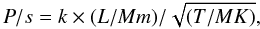 (2)where k ≈ 13 for the global mode and k ≈ 6.7 for its second harmonics, L is the loop length, and T is the average temperature in the loop.
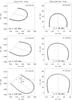 |
Fig. 3 Apparent flare loop axes in the observer’s coordinate system extracted from NoRH images (left column) and their deprojections in the loop plane coordinate system (right column) at three different times depicted in the plots. Loop footpoint baselines and axes of symmetry are shown by dashed lines. |
To estimate the loop length we used a series of 17 GHz images. The apparent loop length, La, is measured along the visible loop axis shown in Fig. 2. The standard deviation for the loop length measurements δ ≈ ±1 Mm (1.4′′). It is well known from the theory of interferometry (see, for example, Thomson et al. 1986) that the error of the definition of the contour level location is significantly less than the interferometer beam size, which is 10′′ for 17 GHz. The accuracy in this case is raised by the signal-to-noise ratio. Because NoRH has high sensitivity, 5 × 10⁻³ sfu in flux density, the signal-to-noise ratio is very high during the flare, not less than 5 for this event.
To obtain values of the deprojected loop length we conducted a loop axis reconstruction using a geometrical technique of Loughhead et al. (1983). This technique is based on coordinates transformation between three natural coordinates systems: observer’s (or image) system, heliographic system, and loop system aligned with the loop plane. Main assumptions of the method that (1) the loop’s central axis lies in a plane and (2) it is symmetrical in its own plane about an axis at right angles to the footpoints baseline are found to be reasonable for the loop examined. The advantage of this method is that it takes into account possible inclination of the loop plane with respect to vertical on the solar surface.
Examples of loop reconstruction for three moments in time are presented in Fig. 3. The visible loop axes in the observer’s coordinate system extracted from 17 GHz NoRH images are shown in the left column. An inclination angle of the loop plane from the vertical state is calculated by measurement of angle ω shown in the left bottom plot. Angle α allows us to calculate a true azimuthal angle between the loop footpoint baseline and the heliographic east-west direction. The corresponding reconstructed axes in the loop plane coordinate system are shown in the right column. Loop lengths corresponding to the apparent axis, La, and to the deprojected axis, L, are depicted in the plots.
The time profiles of an apparent and reconstructed (or deprojected) loop lengths smoothed over 200 s are shown in Fig. 4a. We used the deprojected loop length for estimating the slow magnetoacoustic wave period.
Figure 4b shows the evolution of the plasma temperature, time resolution is 1 min. It is growing during the first microwave peak up to T = 16.7 MK and then gradually decreases. Estimates of the plasma parameters were made from the analysis of the integral soft X-ray fluxes in the two channels 1–8 Å and 0.5–4 Å recorded by GOES. For the calculations we used the standard routine SXT_TEEM. For the GOES measurements, the uncertainties are based on the values given by Garcia (1994): 16% for the long-wavelength GOES channel and 14% for the short-wavelength GOES channel. These values typically result in uncertainties of less than 0.1 MK in temperature.
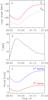 |
Fig. 4 Time profiles of a) loop lengths measured along an apparent (solid line) and deprojected (dashed line) loop axis, b) plasma temperature, and c) periods of the slow magnetoacoustic wave, the global mode (solid line) and its second harmonics (dashed line). |
Time profiles of estimated periods are shown in Fig. 4c for the global mode (solid line) and its second harmonics (dashed line). Both harmonics grow after the time 01:01 UT, which corresponds to the end of the first emission peak in the microwave time profiles. The relative error of the estimate ΔP/P = 0.07.
The estimate of the background plasma density inside the loop n0 and magnetic field strength B in sources are also important. It was shown (Nakariakov & Melnikov 2006) that for a high ratio n0/B in the source the slow magnetoacoustic wave can be observable in microwaves only because of the modulation of the plasma density projected onto the efficiency of the Ruzin suppression of the gyrosynchrotron emission.
The background plasma density can be found using GOES fluxes from the expression for the emission measure:  (3)Taking into account the microwave flaring loop sizes, the deprojected loop length, L(t), and the cross section radius r ≈ 7.5′′, we calculated the volume of the loop as V(t) = πr2L(t). The estimate of the plasma density,
  (4)shows that it grows in the range n0 ≈ 1.5−5.0 × 1010 cm-3 during the flare period.
The analysis of the SOHO/MDI magnetograms shows that on the rise phase of the flare the well-defined round-shaped footpoint sources seen in intensity in Fig. 2a correspond to the magnetic field of opposite polarity with the magnetic field strength Bmin ≈ −1300 G and Bmax ≈ +1800 G on the photosphere level in the areas of the southern and northern sources, respectively.
4. Wavelet analysis
The microwave and hard X-ray signals were processed by means of the wavelet analysis (Torrence & Compo 1998) using the Morlet wavelet that provides a good balance between time and frequency localization.
The information about the spatial structure of the oscillations and their phases in different parts of the flaring loop is important for the MHD mode identification. To obtain this information we used a series of NoRH images at 17 and 34 GHz with the time resolution 2 s.
In Fig. 5a,d,g the time profiles of the flux density at 34 GHz from the southern and northern footpoints and the loop top are shown respectively. Flux densities are calculated from NoRH images by integration of brightness temperature over areas of the size 25′′ × 25′′. Figure 5b,e,h represent the normalized modulation depth for the corresponding sources. The modulation depth of the signal is calculated with Eq. (1). For the wavelet analysis we normalize the value of modulation depth by standard deviation because we are interested mainly in the periodicity in the signal and the period evolution, but not in the modulation depth evolution. The wavelet power spectra are shown in Fig. 5c,f,i. The solid black contour is the 95% confidence level for the red noise. The hatched areas are regions of the wavelet spectrum where edge effects become important, the so called cone of influence.
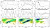 |
Fig. 5 Variations of NoRH flux densities at 34 GHz, normalized modulation depth, and wavelet power spectra for signals from southern FP (a)–c)), northern FP (d)–f)), and loop top (g)–i)). The 95% confidence level on wavelet spectra is shown by the solid black contour. The dashed line shows the calculated period of the second harmonics of the slow magnetoacoustic wave. |
The flux densities from both FPs show emission variations with the modulation depth up to 40% for secondary peaks. Their wavelet power spectra contain a periodic component growing from 2.5 to 4–5 min between 01:00 UT and 01:23 UT. This component appeares immediately after the first emission peak and agrees well with the period of the second harmonics of the slow magnetoacoustic wave shown by the dashed line. The other periodicity within 95% confidence level is 7 min component. It is interesting that the microwave emission from the loop top area does not show obvious flux variation after the first emission peak at both frequencies. Nevertheless, our analysis reveals a shorter periodic component between 01:02 and 01:15 UT and a flux variation with 5% modulation depth.
Figure 6a represents 17 GHz flux density time profiles from the southern (thick line) and northern (thin line) footpoints, as well as from the loop top (dotted line). Wavelet spectra at this frequency (Fig. 6b–d) show periodicities similar to that obtained at 34 GHz. They disappear after 01:22 UT in both footpoints when the magnetic configuration of the microwave loop changed dramatically.
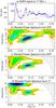 |
Fig. 6 a) Variations of NoRH flux densities at 17 GHz from the southern FP (thick line), northern FP (thin line), and loop top (dotted line). Wavelet power spectra for signals from b) southern FP and c) northern FP and d) loop top. |
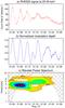 |
Fig. 7 a) Variations of RHESSI hard X-ray signal in 25–50 keV channel and b) its normalized modulation depth; c) wavelet power spectrum of the signal variations. |
The variations of the hard X-ray count rate measured in the RHESSI 25–50 keV channel and its normalized modulation depth are shown in Fig. 7a and b, respectively. The time resolution is 4 s. The wavelet spectrum shown in Fig. 7c is more complicated than for microwave signals. The main periodic component increases from 3.5 to 5 min outside the cone of influence. There is additionally a very short extension on the spectrum with the period about 3 min in the time interval 01:12–01:19 UT and 7 min period.
The same growing periodicity P = 2.5 − 5 min was found from the wavelet analysis of the left and right circular polarized signals (LCP and RCP) detected by NoRH at 17 GHz and from spectral analysis of 17 GHz circular polarisation (V = R − L) integrated over SFP and NFP areas. A 7 min period is also pronounced in these spectra. The wavelet spectra of the pre-flare LCP and RCP signals do not show any spectral components in the range 1–5 min, while the pre-flare RCP signal contains stable 7–8 min pulsations between 23:00 and 24:00 UT on 2005 August 21.
5. Discussion
All analyzed wavelet spectra contain a periodic component that grows with time in the course of the flare. This component agrees well with the calculated period of the second harmonics of the slow magnetoacoustic wave. It appears immediately after the first emission peak and disappears when the magnetic configuration undergoes strong changes: the flare transfers to a different loop system.
It was demonstrated by Nakariakov et al. (2004) that the second standing acoustic harmonics may appear as a natural response of the loop to an impulsive energy deposition located near the loop top. Moreover Tsiklauri et al. (2004) showed that only the second harmonics is excited, regardless of the spatial position of heat deposition. They modeled the evolution of a coronal loop in response to an impulsive heating. It was shown that first, a sudden energy release results in a rapid local increase in the pressure gradient and loop density because of the chromospheric evaporation. The strong impulsively generated pressure disturbance propagates as a slow magnetosonic wave along the loop legs and is reflected at the footpoints finally as a standing wave.
The slow magnetoacoustic wave is perturbing the density of the plasma and the parallel component of the velocity, while the magnetic field remains practically unperturbed by this mode. The density perturbations have a maximum near the loop apex, while longitudinal velocity perturbations have a node there. Therefore, if the microwave emission were influenced by the perturbation of the background density, one would expect to observe the maximum modulation depth of the microwave emission in the loop top. However, we have the opposite situation: the secondary emission peaks are more pronounced in loop footpoints than in the loop top, with the corresponding emission modulation 40% in the FPs and only 5% in the LT.
5.1. Possibility of emission modulation by slow acoustic wave
It is well accepted that microwaves from large solar flares are generated by gyrosynchrotron emission of middle relativistic electrons. The modulation of gyrosynchrotron emission by slow magnetoacoustic oscillations was analyzed by Nakariakov & Melnikov (2006). They showed that this modulation is possible only at frequencies below or comparable to a so-called Razin frequency defined as 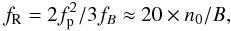 (5)where fp is the plasma frequency and fB is the gyrofrequency in Hz, B is the magnetic field strength in G, and n0 is the background plasma density in cm-3. Therefore, emission modulation works for sufficiently high plasma density or/and low magnetic field. Just after the first peak, at 01:00 UT, the obtained value n0 ≈ 2.8 × 1010 cm-3. With this value for the plasma density we obtain a magnetic field strength near to loop footpoints of B ≈ 32−16 G, which is required for the emission modulation in the frequency range f = 17−34 GHz. It is absolutely impossible to have this low magnetic field strength because |B| > 1000 G on the photospheric level under both footpoints. The centers of the FP boxes for the emission calculation are located about 9000 km (12′′) over the photosphere. The flare frequency spectra reconstructed with Nobeyama Radio Polarimeter data also show that the peak frequency fpeak ≤ 10 GHz during the flare period. This is an additional evidence that the Razin effect is negligible and that therefore in this particular event the variation of the plasma density has no effect on the gyrosynchrotron emission at 17–34 GHz.
Nonthermal hard X-ray emission from large solar flares is the result of thick-target bremsstrahlung of nonthermal electrons that precipitate into the chromosphere near the loop footpoints. The process of precipitation cannot be modulated by the slow acoustic wave either. Therefore, the observed QPP are caused instead by individual episodes of electron acceleration and injection into the coronal loop and not by the modulation of nonthermal electrons via trapping and precipitation.
5.2. Spatial distribution of QPP and modulation depth
The last conclusion agrees well with the minimal emission modulation in the loop top. We suggest that this spatial QPP distribution is not the pulsation mode property, but is connected with the properties of the acceleration and transport of energetic electrons. It was found from the model simulations (Melnikov et al. 2002; Gorbikov & Melnikov 2007; Reznikova et al. 2009) that the absence of the emission peaks in the LT can be a natural consequence of anisotropic injection of accelerated electrons near to the loop apex predominantly along magnetic field lines. In this case the injected electrons pass quickly though the upper part of the loop with almost zero pitch-angle and, therefore, effectiveness of their gyrosynchrotron emission there is very low. We can see from Fig. 6a that after the first emission peak at 17 GHz the flux density from the LT source is four times less then from FP sources.
The modulation depth is found to be up to 40% for microwave QPP in footpoints and 30% for hard X-ray QPP at 25–50 keV. Li & Gan (2008) have found an even higher modulation depth of HXR emission in this flare, which is increasing with the energy up to 90%.
5.3. Periodical triggering of magnetic reconnection
This high modulation depth again indicates that the pulsations in this event are likely to be a manifestation of periodical magnetic reconnection. Chen & Priest (2006) performed MHD numerical simulation of magnetic reconnection and found that the variation of the plasma density in the vicinity of the reconnection site results in a periodic variation in the electron drift speed, which may control the onset of the Buneman or ion-acoustic instability and, therefore, anomalous resistivity. In the model of Nakariakov et al. (2006) quasi-periodic MHD wave-trains can trigger a sharp increase of the electric current density in current sheets, which leads to the generation of plasma micro instabilities and anomalous resistivity. In both models the periodical onset of the anomalous resistivity triggers periodic energy releases.
However, in the event under study, the acoustic waves are supposed to be trapped in the loop, which is already relaxed after the reconnection and does not interact with the reconnecting current sheet. Therefore the question arises of how these waves enter into the current sheet and modulate the magnetic reconnection? The proposed scenario is shown in Fig. 8 and can be described as follows. The second harmonics of the slow mode has a maximum density perturbation at the loop top (Tsiklauri et al. 2004). Because of this and of the action of the centrifugal force arising because of the loop curvature we can expect fast magnetoacousic wave excitation at the loop apex (Verwichte et al. 2006). The fast wave trains generated with the frequency of the second harmonics of the slow mode propagate upward across magnetic field lines and modulate the reconnection rate either by the modulation of the plasma parameters (Chen & Priest 2006), or by a sharp increase of the electric current density in the nearby current sheet (Nakariakov et al. 2006).
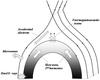 |
Fig. 8 Sketch of the proposed scenario of the QPP excitation in this event. The second harmonics of the slow mode generated by an initial impulsive energy deposition causes the fast magnetoacousic wave excitation at the loop apex, which in turn triggers repeated energy releases in higher loops. The structure of density perturbation along a loop in the second harmonics of the slow magnetoacoustic wave is shown by color. |
Additional evidence for this scenario is the fact that the microwave brightening occurred at slightly different places: the flare loop length and position is changing with time. This implies that different field lines dominate the individual episodes of energy release at different emission peaks, though all field lines belong to the same loop system, which forms the large-scale flare arcade in the corona. This observational fact may also solve a difficulty with the wave dissipation: when the earlier oscillation in one elementary loop is damped and decayed, it is enhanced in another loop of the arcade.
6. Summary and conclusion
We studied QPP during the flare of 2005 August 22 observed with NoRH and RHESSI. Quasi-periodic pulsations in microwaves were analyzed with spatial resolution. This analysis revealed 17 and 34 GHz flux density variation with a modulation depth of up to 40% in both footpoints of the loop and only 5% variation of emission in the loop top. Our analysis of the hard X-ray emission at 25–50 keV shows damped QPP with a modulation depth of up to 30%.
We used a wavelet analysis which allowed us to examine the spectral components in dynamics. All analyzed wavelet spectra show periodic component growing with time during the course of the flare between 2.5 to 5 min. This component agrees well with the period of the second harmonics of the slow magnetoacoustic mode. The calculation of the period takes into account the evolution of a plasma temperature and a flare loop length. The periodicity appears immediately after the first emission peak and disappears when the magnetic configuration of the loop dramatically changed. We did not find any spectral components in the range 1–5 min on the wavelet spectra of the pre-flare LCP and RCP signals at 17 GHz.
Based on these findings we suggest that the second standing harmonics of the slow wave in this event were generated by an initial impulsive energy deposition as proposed by Nakariakov et al. (2004) and Tsiklauri et al. (2004). Strong impulsive pressure disturbances propagate along the loop legs and are reflected at the footpoints to finally form a standing wave.
We exclude the possibility of emission modulation caused by a density variation in the wave. The high modulation depth of the hard X-ray and radio emission indicates that QPP is likely to be a manifestation of periodical magnetic reconnection. Therefore, we suppose that the slow wave excited by the initial energy release may work as a trigger for the repeated energy releases. Owing to the maximum density perturbation at the loop top in the second harmonics of the standing wave and to the action of the centrifugal force in the curved loop one can expect the excitation of fast magnetoacousic waves at the loop apex. The fast wave trains propagating upward across the magnetic field lines can modulate the reconnection rate by periodical onset of the anomalous resistivity through the variation of the plasma parameters or electric current density in the nearby current sheet. In this scenario one period of the slow-mode wave is enough to trigger the next cycle of energy release. Therefore, we do not discuss the dissipative property of the wave.
Acknowledgments
The work was partly supported by RFBR-CNSF grant 08-02-92228, RFBR grant 09-02-00624. The authors are grateful to Prof. Valery Nakariakov and Dr. Victor Melnikov for useful discussions. Wavelet software was provided by C. Torrence and G. Compo, and is available at http://paos.colorado.edu/research/wavelets/. We thank to anonymous referee for a number of useful comments.
References
- Berghmans, D., & Clette, F. 1999, Sol. Phys., 186, 207 [NASA ADS] [CrossRef] [Google Scholar]
- Chen, P. F., & Priest, E. R. 2006, Sol. Phys., 238, 313 [NASA ADS] [CrossRef] [Google Scholar]
- DeForest, C. E., & Gurman, J. B. 1998, ApJ, 501, L217 [NASA ADS] [CrossRef] [Google Scholar]
- De Moortel, I. 2006, Phil. Trans. R. Soc. London Ser. A, 364, 461 [Google Scholar]
- Garcia, H. A. 1994, Sol. Phys., 154, 275 [NASA ADS] [CrossRef] [Google Scholar]
- Gorbikov, S. P., & Melnikov, V. F. 2007, Math. Mod., 19, 112 [Google Scholar]
- Li, Y. P., & Gan, W. Q. 2008, Sol. Phys., 247, 77 [NASA ADS] [CrossRef] [Google Scholar]
- Loughhead, R. E., Wang, J.-L., & Blows, G. 1983, ApJ, 274, 883 [NASA ADS] [CrossRef] [Google Scholar]
- Melnikov, V. F., Shibasaki, K., & Reznikova, V. E. 2002, ApJ, 580, L185 [NASA ADS] [CrossRef] [Google Scholar]
- Mészárosová, H., Karlický, M., Rybák, J., Fárník, F., & Jiřička, K. 2006, A&A, 460, 865 [NASA ADS] [CrossRef] [EDP Sciences] [Google Scholar]
- Nakajima, H., Nishio, M., & Enome, S. 1994, Proc. IEEE, 82, 705 [Google Scholar]
- Nakariakov, V. M., & Melnikov, V. F. 2006, A&A, 446, 1151 [NASA ADS] [CrossRef] [EDP Sciences] [Google Scholar]
- Nakariakov, V. M., & Melnikov, V. F. 2009, Space Sci. Rev., 149, 119 [NASA ADS] [CrossRef] [Google Scholar]
- Nakariakov, V. M., Verwichte, E., Berghmans, D., & Robbrecht, E. 2000, A&A, 362, 1151 [NASA ADS] [Google Scholar]
- Nakariakov, V. M., Tsiklauri, D., Kelly, A., Arber, T. D., & Aschwanden, M. J. 2004, A&A, 414, L25 [NASA ADS] [CrossRef] [EDP Sciences] [Google Scholar]
- Nakariakov, V. M., Foullon, C., Verwichte, E., & Young, N. P. 2006, A&A, 452, 343 [NASA ADS] [CrossRef] [EDP Sciences] [Google Scholar]
- Ofman, L., Nakariakov, V. M., & DeForest, C. E. 1999, ApJ, 514, 441 [NASA ADS] [CrossRef] [Google Scholar]
- Reznikova, V. E., Melnikov, V. F., Shibasaki, K., et al. 2009, ApJ, 297, 735 [NASA ADS] [CrossRef] [Google Scholar]
- Sych, R., Nakariakov, V. M., Karlicky, M., & Anfinogentov, S. 2009, A&A, 505, 791 [NASA ADS] [CrossRef] [EDP Sciences] [Google Scholar]
- Thomson, A. R., Moran, J. M., & Swenson, G. W. 1986, Jr. Interferometry and Synthesis in Radio Astronomy (Wiley-Interscience) [Google Scholar]
- Torrence, C., & Compo, G. P. 1998, Bull. Amer. Meteor. Soc., 79, 61 [CrossRef] [Google Scholar]
- Tsiklauri, D., Nakariakov, V. M., Arber, T. D., & Aschwanden, M. J. 2004, A&A, 422, 351 [NASA ADS] [CrossRef] [EDP Sciences] [Google Scholar]
- Verwichte, E., Foullon, C., & Nakariakov, V. M. 2006, A&A, 449, 769 [NASA ADS] [CrossRef] [EDP Sciences] [Google Scholar]
- Wang, T. J., Solanki, S. K., Curdt, W., et al. 2002, ApJ, 574, L101 [NASA ADS] [CrossRef] [Google Scholar]
- Wang, T. J., Solanki, S. K., Curdt, W., et al. 2003, A&A, 406, 1105 [NASA ADS] [CrossRef] [EDP Sciences] [Google Scholar]
- Wang, T. J., Ofman, L., & Davila, J. M. 2009a, ApJ, 696, 1448 [NASA ADS] [CrossRef] [Google Scholar]
- Wang, T. J., Ofman, L., Davila, J.M., & Mariska, J. T. 2009b, A&A, 503, L25 [NASA ADS] [CrossRef] [EDP Sciences] [Google Scholar]
- Zaitsev, V. V., & Kislyakov, A. G. 2006, Astron. Rep., 50, 823 [NASA ADS] [CrossRef] [Google Scholar]
- Zaitsev, V. V., & Stepanov, A. V. 1989, Sov. Astron. Lett., 15, 66 [NASA ADS] [Google Scholar]
All Figures
|
Fig. 1 Light curves of the flare. a) Soft X-ray in the GOES 1 − 8 Å (thick line) and 0.5 − 4 Å (thin line) channels; b) NoRP flux at 2 GHz (green) and NoRH fluxes integrated over the AR at 17 GHz (blue), and 34 GHz (black); c) hard X-ray count rate measured in RHESSI 25–50 keV channel; d) modulation depth of emission at frequencies 2 GHz (green), 17 GHz (blue), 34 GHz (black) and energy 25–50 keV (red). |
| In the text | |
|
Fig. 2 NoRH images of the flare source at 17 GHz, I at different moments in time. Contours correspond to 0.1, 0.3, 0.5, 0.7, 0.9 levels of maximum |
| In the text | |
|
Fig. 3 Apparent flare loop axes in the observer’s coordinate system extracted from NoRH images (left column) and their deprojections in the loop plane coordinate system (right column) at three different times depicted in the plots. Loop footpoint baselines and axes of symmetry are shown by dashed lines. |
| In the text | |
|
Fig. 4 Time profiles of a) loop lengths measured along an apparent (solid line) and deprojected (dashed line) loop axis, b) plasma temperature, and c) periods of the slow magnetoacoustic wave, the global mode (solid line) and its second harmonics (dashed line). |
| In the text | |
|
Fig. 5 Variations of NoRH flux densities at 34 GHz, normalized modulation depth, and wavelet power spectra for signals from southern FP (a)–c)), northern FP (d)–f)), and loop top (g)–i)). The 95% confidence level on wavelet spectra is shown by the solid black contour. The dashed line shows the calculated period of the second harmonics of the slow magnetoacoustic wave. |
| In the text | |
|
Fig. 6 a) Variations of NoRH flux densities at 17 GHz from the southern FP (thick line), northern FP (thin line), and loop top (dotted line). Wavelet power spectra for signals from b) southern FP and c) northern FP and d) loop top. |
| In the text | |
|
Fig. 7 a) Variations of RHESSI hard X-ray signal in 25–50 keV channel and b) its normalized modulation depth; c) wavelet power spectrum of the signal variations. |
| In the text | |
|
Fig. 8 Sketch of the proposed scenario of the QPP excitation in this event. The second harmonics of the slow mode generated by an initial impulsive energy deposition causes the fast magnetoacousic wave excitation at the loop apex, which in turn triggers repeated energy releases in higher loops. The structure of density perturbation along a loop in the second harmonics of the slow magnetoacoustic wave is shown by color. |
| In the text | |
Current usage metrics show cumulative count of Article Views (full-text article views including HTML views, PDF and ePub downloads, according to the available data) and Abstracts Views on Vision4Press platform.
Data correspond to usage on the plateform after 2015. The current usage metrics is available 48-96 hours after online publication and is updated daily on week days.
Initial download of the metrics may take a while.