| Issue |
A&A
Volume 525, January 2011
|
|
|---|---|---|
| Article Number | A124 | |
| Number of page(s) | 12 | |
| Section | Galactic structure, stellar clusters and populations | |
| DOI | https://doi.org/10.1051/0004-6361/201015510 | |
| Published online | 07 December 2010 | |
High resolution HDS/SUBARU chemical abundances of the young stellar cluster Palomar 1⋆
1
European Southern Observatory,
Casilla 19001,
Santiago,
Chile
e-mail: This email address is being protected from spambots. You need JavaScript enabled to view it.
2
Istituto Nazionale di Astrofisica – Osservatorio Astronomico di
Bologna, via Ranzani 1, 40127
Bologna,
Italy
3
GEPI, Observatoire de Paris, CNRS, Université Paris Diderot,
Place Jules
Janssen, 92190
Meudon,
France
4
Istituto Nazionale di Astrofisica – Osservatorio Astronomico di
Trieste, via G. B. Tiepolo 11, 34143
Trieste,
Italy
5
Universidad de Concepción, Casilla 160-C, Concepción, Chile
Received: 1 August 2010
Accepted: 21 October 2010
Abstract
Context. Palomar 1 is a peculiar globular cluster (GC). It is the youngest Galactic GC and it has been tentatively associated to several of the substructures recently discovered in the Milky Way (MW), including the Canis Major (CMa) overdensity and the Galactic Anticenter Stellar Structure (GASS).
Aims. In order to provide further insights into its origin, we present the first high resolution chemical abundance analysis for one red giant in Pal 1.
Methods. We obtained high resolution (R = 30 000) spectra for one red giant star in Pal 1 using the high dispersion spectrograph (HDS) mounted at the SUBARU telescope. We used ATLAS-9 model atmospheres coupled with the SYNTHE and WIDTH calculation codes to derive chemical abundances from the measured line equivalent widths of 18 among α, Iron-peak, light and heavy elements.
Results. The Palomar 1 chemical pattern is broadly compatible to that of the MW open clusters population and similar to disk stars. It is, instead, remarkably different from that of the Sagittarius (Sgr) dwarf spheroidal galaxy.
Conclusions. If Pal 1 association with either CMa or GASS will be confirmed, this will imply that these systems had a chemical evolution similar to that of the Galactic disk.
Key words: stars: abundances / Galaxy: abundances / globular clusters: individual: Palomar 1
Appendix is only available in electronic form at http://www.aanda.org, and also at the CDS via anonymous ftp to cdsarc.u-strasbg.fr (130.79.125.5) or via http://cdsarc.u-strasbg.fr/viz-bin/qcat?J/A+A/525/A124
© ESO, 2010
1. Introduction
Palomar 1 is sparsely populated and the youngest among Galactic globular clusters (MV = −2.5 ± 0.5; age = 6.3–8 Gyr, Rosenberg et al. 1998a, hereafter R98a). Very little is known on this cluster: Rosenberg et al. (1998b, hereafter R98b) provided the only spectroscopic study of Pal 1 red giant branch stars to date. By observing four stars in the calcium II Triplet infrared region, they derived a systemic heliocentric velocity of vhelio = −82.8 ± 3.3 km s-1 and a metallicity [Fe/H] = −0.71 ± 0.20. Besides its unusual age and metallicity, the global slope of the Pal1 mass function (MF) is flatter than Galactic globular clusters (GCs) at similar locations and, hence, it does not fit the correlation with Galactic position (RGC, ZGP), and metallicity [Fe/H] followed by old Milky Way (MW) GCs (see Fig. 12 in R98a; and Djorgovski et al. 1993). R98a considered also the possibility of Pal 1 being an open cluster (OC). The concentration derived, c = 1.6, higher than any OC, and its position in the Galaxy (RGC = 17.3,Z = 3.6 kpc) would make it a peculiar OC, though. Its mass and half light radius place Pal 1 among the “lucky survival” in the vital diagram of GCs (Gnedin & Ostriker 1997). This suggests that Pal 1 has lost an important fraction of its mass. In fact, R98a calculate an evaporation time of 0.74 Gyr and concluded that Pal1 might be on the verge of destruction.
Basic parameters of Pal1-I. Measured radial velocity and spectra signal-to-noise ratios are also reported.
Several authors suggested that young GCs like Pal l may be related to dwarf satellites disrupted in the early stages of formation of the MW (see, e.g., Lynden-Bell & Lynden-Bell 1995) and it is now clear that accreted satellites might have in fact contributed to the star clusters population of the Galactic halo and likely also to the disk OCs population (e.g. Frinchaboy et al. 2004; Carraro & Bensby 2009; Law & Majewski 2010).
Indeed, putative association of Pal 1 with several of the substructures discovered in the Galactic halo over the past decade has been suggested. In particular, association of Pal 1 with the “GASS” (Galactic Anticenter Stellar Structure. Crane et al. 2003; Frinchaboy et al. 2004) and the controversial Canis Major dSph galaxy (Momany et al. 2006; Martin et al. 2004; Forbes & Bridges 2010) have been proposed. Association with the “orphan stream” (Belokurov et al. 2007) was also suggested, although a recent study of the stream orbit argue against this possibility (Newberg et al. 2010). While Pal 1 seems not to be related with the Sagittarius (Sgr) dwarf spheroidal galaxy tidal streams (Law & Majewski 2010) either, it is interesting to notice that Pal 1 comfortably fits into the Sgr age vs. metallicity relation (AMR) derived by Siegel et al. (2007). Pal 1 and the young Sgr GCs Ter 7 and Pal 12, are also the only three GCs having [Fe/H] > −1.2 and lying at Galactocentric distances RGC > 8 kpc.
Recently, Niederste-Ostholt et al. (2010) detected tidal tails out to a distance of about 90 rh (~1 degree) from either side of Pal 1. They argue that Pal 1 might have been evolving in a dwarf galaxy accreted by the MW less than 500 Myr ago.
Chemical abundance patterns provide information about the formation history of the system in which stars were formed. In particular, the MW satellites and their GCs systems present chemical compositions remarkably different from what observed in the MW (see, e.g. Venn et al. 2004; Monaco et al. 2005; Lanfranchi et al. 2006; Monaco et al. 2007; Sbordone et al. 2007). In order to shed light onto its origin, we present here the first high resolution chemical abundance analysis for a red giant star in the peculiar GC Palomar 1.
2. Observations and data reductions
We observed the Red Giant Branch (RGB) star Pal1-I (according to the nomenclature introduced in R98b) using the High Dispersion Spectrograph (HDS, Noguchi et al. 2002) mounted at the SUBARU telescope in Mauna Kea (Hawaii). The Pal 1 RGB contains very few stars (see, e.g., Fig. 1 in R98b) and, although more stars were in our target list, only this one could be eventually observed. While having only one star may be a concern, the homogeneity of the iron abundances of all stars measured by R98b suggest that Pal 1-I is likely not a peculiar object. Yet, the presence of a spread in the measured abundance ratios is an issue which cannot be addressed in the present analysis.
Two 1 h exposures were taken on November 2nd 2007 in service mode (Progr.ID: S07A-144S) using the standard StdYb setup which covers the spectral range ~4100–6900 Å. For each exposure, the entire spectral range is recorded in two frames through a blue and a red CCD. We adopted a 1.2″ slit width which provides a spectral resolution of R = 30 000.
We employed the overscan region to perform the bias subtraction with the aid of in-house script available from the HDS/SUBARU web page1. To remove cosmic rays we used IRAF2 scripts available at the same URL. We applied a median filter to the data and compared the counts to the original frames. When high peaks were detected the pixels values were substituted with the counts of the median-filtered image. The procedure is described in Aoki et al. (2005).
Data reduction was performed using standard IRAF tasks and included order tracing, flat-fielding, background and sky subtraction and extraction. Standard Th-Ar arcs were used for wavelength calibrations. The four scientific frames were reduced individually.
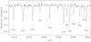 |
Fig. 1 Sample of the spectrum obtained for Pal1-I. Lines corresponding to different elements are marked in the figure. |
The object radial velocity (RV) was computed for each frame by cross-correlating the observed spectra with a synthetic one of similar atmospheric parameter using the IRAF task fxcor. Finally, the single exposure spectra were reduced at rest frame and averaged. The final spectrum has a signal to noise of ~40 at 560 nm. The IRAF task rvcorrect was used to calculate the earth motion and convert the observed RV to the heliocentric system. Figure 1 shows a sample of the obtained spectrum.
Table 1 reports Pal1-I coordinates, magnitudes from R98b, S/N and the measured radial velocity. The reported RV (−76.1 km s-1) is the average of the measures in the 4 frames available. The standard deviation of the four derived RVs is ~0.2 km s-1. HDS is located at a Nasmyth platform and, as such, should not be critically affected by flexures. However, by measuring a few sky lines we evaluate a residual uncertainty in the RV of the order of an additional <0.2 km s-1. We adopted a conservative 0.5 km s-1 estimate for the RV error. For Pal1-I, R98b obtained vhelio = −81.0 ± 4.6 km s-1 from lower resolution spectra (R ≃ 4000) centered on the Ca II triplet. Clearly, the two measures are compatible with each other within 1-σ.
We remark here that R98a also acquired control fields and showed that the region of color–magnitude diagram (CMD) in which Pal 1-I is selected is virtually free from field stars contamination (see Fig. 5 in R98a). This is confirmed by the Galaxy model of Robin et al. (2003)3 which predicts 1 × 10⁻³ stars in a 80″ region centered on Pal 1 (Pal 1-I lies at about 49″ from the cluster center) in a CMD box defined by 1.11 < (V − I) < 1.21; 16.09 < V < 16.69 and having radial velocity in the range −80 < vhelio(km s-1) < −70. The above figure raises to 7 × 10⁻² if we consider the whole cluster region out to the tidal radius (rt = 525″, R98a). Therefore, Pal 1-I is unlikely to be a field star.
3. Chemical abundance analysis
3.1. Linelist and equivalent width measurements
Species abundances are obtained from line equivalent widths (EWs) measured using the DAOSPEC code. The Gaussian approximation adopted by DAOSPEC represents a reliable approximation to the line profile at the resolution under consideration up to relatively strong lines (~150 mÅ, see Stetson & Pancino 2008; Pancino et al. 2010).
Appendix A reports the adopted linelist, atomic parameters and measured line EWs. Atomic parameters were retrieved from the Vienna Atomic Line Database (VALD4, Kupka et al. 2000) with the exception of the single lines measured for Mn and Co. Both these elements are known to be significantly affected by hyperfine splitting. For these transitions we adopted the hyperfine structures (HFS) tabulated by Prochaska et al. (2000).
In order to perform a differential solar analysis, we broadened the Kurucz (2005) Solar Flux Atlas5 to the resolution of our SUBARU Pal1-I spectrum (R = 30 000) and measured the solar line EWs (see Appendix A) as above.
Silicon solar abundances calculated adopting VALD log gf present a large dispersion. This may imply an important level of internal inconsistency among these log gf. Therefore, for Si lines we adopted the oscillator strengths of Bensby et al. (2009).
3.2. Model atmospheres and chemical abundances
An initial estimate of the atmospheric parameters was obtained from the R98b Pal1-I photometry (see Table 1). Adopting a reddening of E(B − V) = 0.15 (Harris 1996), we obtain an effective temperature of Teff = 4820 K from the Alonso et al. (1999) calibrations for the Pal1-I (V − I) color. We note that the Schlegel et al. (1998, hereafter SFD98) reddening maps provide a significantly larger reddening value, E(B − V) = 0.19, which implies Teff = 4950 K. However, by applying the Bonifacio et al. (2000) correction to SFD98 reddening values larger than E(B − V) = 0.10, we obtain E(B − V) = 0.16 and, correspondingly, Teff = 4850 K.
Adopting ages between 4 and 8 Gyr and a metallicity of Z = 0.004 (Rosenberg et al. 1998a), we derived a gravity of log g = 2.4 ± 0.5 dex by comparison with the Girardi et al. (2002) and the Pietrinferni et al. (2004) isochrones.
A first model atmosphere having the above parameters and [M/H] = −0.5 was computed using the Linux port of version 9 of the ATLAS code and abundances were derived from the line EWs using the WIDTH code (Kurucz 1993a; Sbordone et al. 2004). Iron lines were used to refine the atmospheric parameters. The microturbulence velocity (ξ) was estimated by minimizing the dependence of the abundances from the measured EWs. The effective temperature is determined by imposing that abundances should be independent from the transition excitation potential. We finally adopt a slightly hotter temperature of Teff = 5000 K for Pal1-I. Iron abundances derived by Fe I and Fe II lines provide an excellent agreement, confirming the photometric gravity as a proper value.
For the Sun, Fe abundances calculated adopting a model atmosphere having [M/H] = 0 and the standard solar effective temperature and gravity (Teff = 5777 K, log g = 4.44 ) satisfy well the above requirements, while for the microturbulence we obtain ξ = 0.9 km s-1, well within the range of figures adopted in the literature (see for instance Prochaska et al. 2000; Bensby et al. 2009).
Atmospheric parameters adopted for Pal1-I and the Sun.
Table 2 summarizes the atmospheric parameters adopted for Pal1-I and the Sun. Model atmospheres having these parameters were calculated and employed within the WIDTH code to derive the species abundances from the measured EWs for all elements but Mn and Co. For these elements the abundances were obtained by comparing the measured EWs to that of synthetic lines calculated with the SYNTHE code along with the HFS presented in Prochaska et al. (2000). The abundances obtained for each line are reported in Appendix A. Table 3 presents the average abundances obtained for each species both for the Sun and Pal1-I. In the last two column we report the solar abundances of Grevesse & Sauval (1998, hereafter GS98) and the difference with the present analysis. While for several elements we obtain a good agreements with GS98, we also find notable discrepancies in a few elements. This is not uncommon in differential abundance analysis (see, e.g., Prochaska et al. 2000; Bensby et al. 2003, 2009; Pancino et al. 2010). In particular, we find high discrepancies in the derived Al (−0.25 dex) and Y (+0.43 dex) abundances. The two Al lines measured here (6696 Å and 6698 Å) are known to give systematically lower abundances and, in fact, several authors adopt astrophysical values of the oscillator strengths (see, e.g., Bensby et al. 2003, hereafter B03). We measured only one Y line, which is also known to provide abundances higher than other lines (see B03). The two La lines measured in the Pal1-I spectrum were not detected in the Sun. As such, for La we adopt the GS98 solar value.
Average elemental abudances measured for both Pal1-I and the Sun.
In the following, the Pal1-I abundances will be always referred to our own solar abundances. The measured Pal1-I abundances with respect to solar are also reported in Table 3, as well as the dispersion (σ) of the abundances. It is common practice to report, instead of σ, the standard deviation of the mean of the abundances, i.e. the σ values divided by the square root of the number of lines used (σ/ ). However, this is a safe procedure only by assuming that each line provides an independent measure of the element abundance and we prefer to report, instead, the σ values obtained.
We measure for Pal 1-I an Iron content of [Fe/H] = −0.49 ± 0.18. This is perfectly compatible with the measures of R98b ([Fe/H] = −0.71 ± 0.20).
Expected errors in the Pal1-I abundances due to estimated uncertainties in the atmospheric parameters.
We report in Table 4 the changes in the abundances expected for variations in the atmospheric parameters of (ΔTeff = ± 100 K; Δlog g = ± 0.50; Δξ = ± 0.10 km s-1), i.e. compatible with their estimated uncertainty.
4. Discussion
In the ideal case, we would like to compare the Pal 1 abundance pattern to the outcome of a self-consistent evolutionary model. Existing models however are not yet able to return abundance ratios as detailed as the ones we can measure observationally (see, e.g., a review in Gnedin 2010). To gain some insight into the possible origin of this cluster, we thus follow the common practice of comparing its abundance ratios to those of other stellar systems. This is further justified because abundances might be inherited, at least partially, from the pre-enriched interstellar medium of a host system. Because both Galactic and extra-galactic origins were postulated in the past for Pal 1, these two possibilities are examined separately in the next sections.
4.1. Pal 1 as a Galactic cluster
The iron abundance of Pal 1 is typical of the thick disk, whose distribution peaks around –0.7 (Ivezić et al. 2008), and it is on the tail of the distribution of the thin disk, which peaks around –0.15 (Holmberg et al. 2007). This metallicity is among the highest found in globular clusters and among the lowest found in open clusters. Thus, from the point of view of its iron content, it is difficult to classify Pal 1.
The ratio of α elements to iron (Fig. 2) is essentially solar. From this point of view Pal 1 is like thin disk stars and Open Clusters, but markedly different from thick disk stars, which show enhanced α to iron ratios (Fuhrmann 2008, and references therein). Note however, that from the data of Fuhrmann (2008), at the metallicity of Pal 1 the thin disk already displays an α element enhancement, [Mg/Fe] ~ +0.2.
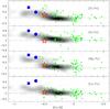 |
Fig. 2 Pal1-I (big empty red star) α-element abundance ratios are presented together with thick and thin Galactic disk stars (shaded area) from Reddy et al. (2006, 2003). Also plotted are the Galactic OCs from Pancino et al. (2010) and the literature compilation presented in that study (filled green circles) and the GCs 47 Tuc (big filled blue squares) and M 71 (big filled pentagon) from Koch & McWilliam (2008), Ramírez & Cohen (2002). The OCs Be 22, Be 29 and Tom 2 are also marked by a plus symbol. |
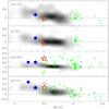 |
Fig. 3 Pal1-I (big empty red star) light odd elements abundance ratios. Other symbols are the same as in Fig. 2. |
The light odd elements (Na and Al, see Fig. 3), that are usually associated to nucleosynthesis by proton captures, both show a moderate enhancement. Both Bensby et al. (2005) and Reddy et al. (2006) noted that in disk stars Na and Al have opposite trends with metallicity, while Al behaves like α elements becoming enhanced with decreasing metallicity, Na is flat around [Na/Fe] = +0.1. Bensby et al. (2005) even claim a significative difference between thin and thick disk, the thin disk being slightly more Na enhanced. The [Na/Fe] = +0.38 found by our analysis is at odds, by a factor of 2 with the mild Na enhancement found in disk stars. The [Al/Fe] = +0.25 is, instead perfectly in line with the increase of this ratio with decreasing metallicity. Incidentally this puts Pal 1 exactly between the thin and thick disk, at this metallicity (see Fig. 8 of Bensby et al. 2005). One should question if this overabundance of Na is real or if it is linked to differential non-local thermodynamic equilibrium (NLTE) effects between this giant in Pal 1 and the dwarf and sub-giant stars analyzed by Bensby et al. (2005) and Reddy et al. (2003, 2006). According to the NLTE computations of Gratton et al. (1999) a corrections of the order of ≃ –0.1 dex should be applied to both our Pal 1 and solar abundances, leaving, hence, the [Na/Fe] abundance ratio practically unchanged. The Na abundances in disk dwarfs and subgiants were derived by Reddy et al. (2003, 2006) using the 615 nm, 616 nm lines while Bensby et al. (2005) used also the same lines adopted by us. In both these cases the NLTE corrections have been considered to be small and were not included in the analysis. It thus appears unlikely that the high Na abundance we derive, is due to differential NLTE effects between dwarfs and giants.
Another thing to be considered is whether the high Na abundance is indeed a chemical signature of Pal 1 or if it has to be understood in terms of the Na-O anti-correlation found in Globular Clusters (Carretta et al. 2009, and references therein). In Globular Clusters the “unpolluted” stars have [O/Fe] ~ +0.5 and [Na/Fe] ~ −0.3 (see Fig. 6 of Carretta et al. 2009), a “polluted” star, with [Na/Fe] = +0.4 can have an oxygen to iron ratio which is 1 dex below this. Given that in Pal 1-I the α to iron ratios are solar, we expect [O/Fe] to be significantly sub-solar. However this possibility cannot be checked, because the only measurable oxygen line – [O I] 630 nm – is in our spectra superimposed to a telluric line and is, therefore, not suited for abundance analysis.
The other odd light elements measured, Sc and V, may have a production channel by proton captures, but may be also produced in nuclear statistical equilibrium, like other iron-peak elements. In Pal 1 their ratio to iron appears solar, like it is in disk stars.
Among the other iron-peak elements (Fig. 4) what stands out are the underabundance of Cr and the overabundance of Zn. For Cr one should be aware of the possible NLTE effects, as are found in metal-poor stars (Bonifacio et al. 2009; Bergemann & Cescutti 2010). For Zn, according to the computations of Takeda et al. (2005) the NLTE correction should be only of the order of −0.1 dex. It is anyway remarkable that for both these elements the ratio to iron appears similar to what found in the Globular Cluster M71 (Ramírez & Cohen 2002). Therefore it is likely that these ratios are specific signatures of Pal 1.
For neutron capture elements (Fig. 5) the most relevant feature, with respect to disk stars of similar metallicities, is the underabundance of Y and overabundance of Ba. It is tempting to interpret this as an overabundance of second-peak s-process elements (Ba), to light s-process elements (Y) as can be expected when the s-process is dominated by moderately metal-poor stars (see Busso et al. 1999, and references therein).
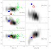 |
Fig. 4 Pal1-I (big empty red star) abundance ratios for Fe-peak elements. Other symbols are the same as in Fig. 2. |
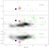 |
Fig. 5 Pal1-I (big empty red star) heavy element abundance ratios. Other symbols are the same as in Fig. 2. |
4.2. The possible extra-galactic origin of Pal 1
Because Pal 1 is peculiar in terms of age and metallicity compared to other GCs, a number of studies tried to associate it to different Galactic sub-structures. In particular, Frinchaboy et al. (2004) proposed the GASS, and Forbes & Bridges (2010) proposed the putative CMa dwarf (see also Martin et al. 2004). In view of the ambiguous nature of these two structures, we add also the Sagittarius dSph galaxy to the set of template extra-galactic systems: it is the only galaxy with measured abundance ratios, and whose metallicity reaches values as high as that of Pal 1 (Monaco et al. 2005; Sbordone et al. 2007).
Therefore in Figs. 6 to 8 we show again the abundance ratios of Pal 1-I, but this time compared to Sagittarius dSph stars from Sbordone et al. (2007, hereafter S07), stars in the GCs Pal 12 and Ter 7 (likely associated to Sgr, Cohen 2004; and S07), stars in the CMa overdensity region (Sbordone et al. 2005) and stars in the GASS (Chou et al. 2010).
Chou et al. (2010) have recently, presented Ti, La and Y abundances for 21 M-giants in the GASS (open diamonds in Figs. 6 and 7). Pal 1 presents Ti and Y content compatible with them, while the La abundance is remarkably different. Detailed chemical abundances for more stars in Pal 1 and for additional elements for stars in the GASS are required to reliably assess the compatibility of the two chemical patterns. At the present stage, we can only conclude that the association of Pal 1 and the GASS is not supported by our abundance analysis. The AMR of the GASS was derived by Frinchaboy et al. (2004) using both GCs and OCs belonging to the area of interest. Some of the OCs they considered, namely Be 22, Be 29 and Tom 2, have measured abundances and are included in Figs. 2–5 (plus symbols). These OCs have abundance patterns qualitatively not dissimilar with respect to the rest of the OCs plotted in the figures, which are also similar to Pal 1.
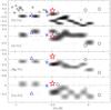 |
Fig. 6 Pal1-I (big empty red star) α-element abundance ratios are presented together with Sagittarius dSph stars (grey shaded area) from S07, and stars in the GCs Pal 12 (big open blue triangle) and Ter 7 (big blue asterisk) from Cohen (2004) and S07, respectively. Stars in the CMa overdensity region in the background of the OC NGC 2477 are plotted as big open circles (Sbordone et al. 2005). M-giants in the GASS from Chou et al. (2010) are plotted as open diamonds. |
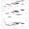 |
Fig. 7 Pal1-I (big empty red star) heavy element abundance ratios. Other symbols are the same as in Fig. 6. |
Data are definitely more sparse for the case of CMa. To date only three giant stars in the background of the OC NGC 2477 were studied (Sbordone et al. 2005, hereafter S05, big open circles in the Figs. 6, 7). S05 suggested that the CMa structure should have undergone a level of chemical processing compatible with that of the Galactic disk. Because Pal 1 chemical properties are also compatible with those of the disk, an association to CMa might be possible. Indeed, the most metal-poor among the stars studied in S05 has an iron content similar to Pal 1-I ([Fe/H] = −0.42) and the chemical composition of the two objects is also quite similar, particularly in the α elements and neutron capture elements (see Figs. 6, 7).
We also compare with the Sgr dSph, which, as mentioned above, is the only among MW satellite to have a mean metallicity similar to that of Pal 1 (Monaco et al. 2002, 2005). Sgr stars studied by Sbordone et al. (2007, hereafter S07) are plotted in Figs. 6, 7 as a gray shaded area. The GCs Ter 7 (S07, big asterisk) and Pal 12 (Cohen 2004, big open triangle) are also plotted since they are believed to belong to the Sgr GCs system, either in the main body (Ter 7) or in the Sgr trailing tail (Pal 12). There are some remarkable similarities of Pal 1 abundances with Ter 7 for α elements and neutron capture elements (Figs. 6, 7). For the latter there is a similarity also with the Sgr field stars. The sodium overabundance seems however a distinctive feature of Pal 1-I (Fig. 8). Additionally, Pal 1 does not show the peculiar Sgr Iron-peak and light odd elements (Figs. 9 and 8) abundance ratios.
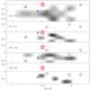 |
Fig. 8 Pal1-I (big empty red star) light odd elements abundance ratios. Other symbols are the same as in Fig. 6. |
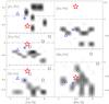 |
Fig. 9 Pal1-I (big empty red star) abundance ratios for Fe-peak elements. Other symbols are the same as in Fig. 6. |
5. Conclusion
We have presented the first high resolution chemical abundances of 18 among α, Iron-peak, light and heavy elements for one giant in the peculiar, young cluster Palomar 1. Pal 1 chemical abundance pattern is similar to that of the Galactic OCs population and significantly different from that of stars in the Sgr dwarf spheroidal galaxy. The different chemical composition with respect to stars analyzed in the GASS, would argue against the associations of Pal 1 with this structure. More data is, however, needed to reliably assess the compatibility of the two systems chemical patterns. If the association between Pal 1 and CMa will be proved, this would imply that the CMa overdensity has undergone a degree of chemical processing similar to the Galactic disk, in agreement with Sbordone et al. (2005).
Pal 1 might then be a GC which experienced a peculiar chemical evolution or an OC ejected from the Galactic disk, which high concentration and flat MF would be the result of its peculiar dynamical evolution. Only a reconstruction of the cluster’s orbit would permit discriminating between the two possibilities. In this respect we remark that, as pointed out by Peñarrubia et al. (2005), radial velocities and positions are not sufficient to claim a common orbit; measurements of proper motions are needed to break degeneracies. A measure of the Pal 1 proper motion is therefore crucial to disentangle the origin of this peculiar system.
Online material
Appendix A: Individual line data
The following table reports the line list and atomic parameters adopted for Pal1-I and the Sun. For the Mn and Co lines we adopted the HFS of Prochaska et al. (2000). The measured equivalent width and the corresponding abundance obtained for each line are also reported.
Adopted line list and atomic parameters. The measured equivalent width and the corresponding abundances obtained for each line are also reported for both Pal1-I and the Sun.
IRAF is distributed by the National Optical Astronomy Observatories, which is operated by the association of Universities for Research in Astronomy, Inc., under contract with the National Science Foundation.
Acknowledgments
We would like to thank Elena Pancino for providing the literature open clusters data used in Figs. 2–5 in electronic format and for useful discussion about the DAOSPEC code.
References
- Alonso, A., Arribas, S., & Martínez-Roger, C. 1999, A&AS, 140, 261 [NASA ADS] [CrossRef] [EDP Sciences] [Google Scholar]
- Aoki, W., Honda, S., Beers, T. C., et al. 2005, ApJ, 632, 611 [NASA ADS] [CrossRef] [Google Scholar]
- Belokurov, V., Evans, N. W., Irwin, M. J., et al. 2007, ApJ, 658, 337 [Google Scholar]
- Bensby, T., Feltzing, S., & Lundström, I. 2003, A&A, 410, 527 [NASA ADS] [CrossRef] [EDP Sciences] [Google Scholar]
- Bensby, T., Feltzing, S., Lundström, I., & Ilyin, I. 2005, A&A, 433, 185 [NASA ADS] [CrossRef] [EDP Sciences] [Google Scholar]
- Bensby, T., Johnson, J. A., Cohen, J., et al. 2009, A&A, 499, 737 [NASA ADS] [CrossRef] [EDP Sciences] [Google Scholar]
- Bergemann, M., & Cescutti, G. 2010, A&A, 522, A9 [NASA ADS] [CrossRef] [EDP Sciences] [Google Scholar]
- Bonifacio, P., Monai, S., & Beers, T. C. 2000, AJ, 120, 2065 [NASA ADS] [CrossRef] [Google Scholar]
- Bonifacio, P., Spite, M., Cayrel, R., et al. 2009, A&A, 501, 519 [NASA ADS] [CrossRef] [EDP Sciences] [Google Scholar]
- Busso, M., Gallino, R., & Wasserburg, G. J. 1999, ARA&A, 37, 239 [NASA ADS] [CrossRef] [Google Scholar]
- Carraro, G., & Bensby, T. 2009, MNRAS, 397, L106 [NASA ADS] [CrossRef] [Google Scholar]
- Carretta, E., Bragaglia, A., Gratton, R., & Lucatello, S. 2009, A&A, 505, 139 [NASA ADS] [CrossRef] [EDP Sciences] [Google Scholar]
- Chou, M.-Y., Majewski, S. R., Cunha, K., et al. 2010, ApJ, 702, L5 [NASA ADS] [CrossRef] [Google Scholar]
- Cohen, J. G. 2004, AJ, 127, 1545 [NASA ADS] [CrossRef] [Google Scholar]
- Crane, J. D., Majewski, S. R., Rocha-Pinto, H. J., et al. 2003, ApJ, 594, L119 [NASA ADS] [CrossRef] [Google Scholar]
- Djorgovski, S., Piotto, G., & Capaccioli, M. 1993, AJ, 105, 2148 [NASA ADS] [CrossRef] [Google Scholar]
- Forbes, D. A., & Bridges, T. 2010, MNRAS, 404, 1203 [NASA ADS] [Google Scholar]
- Frinchaboy, P. M., Majewski, S. R., Crane, J. D., et al. 2004, ApJ, 602, L21 [NASA ADS] [CrossRef] [Google Scholar]
- Fuhrmann, K. 2008, MNRAS, 384, 173 [NASA ADS] [CrossRef] [Google Scholar]
- Girardi, L., Bertelli, G., Bressan, A., et al. 2002, A&A, 391, 195 [NASA ADS] [CrossRef] [EDP Sciences] [Google Scholar]
- Gnedin, O. Y. 2010, in IAU Symp., 270, Computational Star Formation, Barcelona, June 2010 [arXiv:1010.3707] [Google Scholar]
- Gnedin, O. Y., & Ostriker, J. P. 1997, ApJ, 474, 223 [NASA ADS] [CrossRef] [Google Scholar]
- Gratton, R. G., Carretta, E., Eriksson, K., & Gustafsson, B. 1999, A&A, 350, 955 [NASA ADS] [Google Scholar]
- Grevesse, N., & Sauval, A. J. 1998, Space Sci. Rev., 85, 161 [NASA ADS] [CrossRef] [Google Scholar]
- Harris, W. E. 1996, AJ, 112, 1487 [NASA ADS] [CrossRef] [Google Scholar]
- Holmberg, J., Nordström, B., & Andersen, J. 2007, A&A, 475, 519 [NASA ADS] [CrossRef] [EDP Sciences] [MathSciNet] [Google Scholar]
- Ivezić, Ž., Sesar, B.; Jurić, M. et al. 2008, ApJ, 684, 287 [NASA ADS] [CrossRef] [Google Scholar]
- Koch, A., & McWilliam, A. 2008, AJ, 135, 1551 [NASA ADS] [CrossRef] [Google Scholar]
- Kupka, F. G., Ryabchikova, T. A., Piskunov, N. E., Stempels, H. C., & Weiss, W. W. 2000, Balt. Astron., 9, 590 [NASA ADS] [Google Scholar]
- Kurucz, R. L. 2005, Mem. Soc. Astron. Ital. Supp., 8, 189 [Google Scholar]
- Kurucz, R. L. 1993a, CD-ROM 13, 18, http://kurucz.harvard.edu [Google Scholar]
- Lanfranchi, G. A., Matteucci, F., & Cescutti, G. 2006, A&A, 453, 67 [NASA ADS] [CrossRef] [EDP Sciences] [Google Scholar]
- Law, D. R., & Majewski, S. R. 2010, ApJ, 718, 1128 [NASA ADS] [CrossRef] [Google Scholar]
- Lynden-Bell, D., & Lynden-Bell, R. M. 1995, MNRAS, 275, 429 [NASA ADS] [Google Scholar]
- Martin, N. F., Ibata, R. A., Bellazzini, M., et al. 2004, MNRAS, 348, 12 [NASA ADS] [CrossRef] [Google Scholar]
- Momany, Y., Zaggia, S., Gilmore, G., et al. 2006, A&A, 451, 515 [NASA ADS] [CrossRef] [EDP Sciences] [Google Scholar]
- Monaco, L., Ferraro, F. R., Bellazzini, M., & Pancino, E. 2002, ApJ, 578, L47 [NASA ADS] [CrossRef] [Google Scholar]
- Monaco, L., Bellazzini, M., Bonifacio, P., et al. 2005, A&A, 441, 141 [NASA ADS] [CrossRef] [EDP Sciences] [MathSciNet] [Google Scholar]
- Monaco, L., Bellazzini, M., Bonifacio, P., et al. 2007, A&A, 464, 201 [NASA ADS] [CrossRef] [EDP Sciences] [Google Scholar]
- Newberg, H. J., Willett, B. A., Yanny, B., & Xu, Y. 2010, ApJ, 711, 32 [NASA ADS] [CrossRef] [Google Scholar]
- Niederste-Ostholt, M., Belokurov, V., Evans, N. W., et al. 2010, MNRAS, 408, L66 [NASA ADS] [Google Scholar]
- Noguchi, K., Aoki, W., Kawanomoto, S., et al. 2002, PASJ, 54, 855 [NASA ADS] [CrossRef] [Google Scholar]
- Palma, C., Kunkel, W. E., & Majewski, S. R. 2000, PASP, 112, 1305 [NASA ADS] [CrossRef] [Google Scholar]
- Pancino, E., Carrera, R., Rossetti, E., & Gallart, C. 2010, A&A, 511, A56 [NASA ADS] [CrossRef] [EDP Sciences] [Google Scholar]
- Peñarrubia, J., Martínez-Delgado, D., Rix, H. W., et al. 2005, ApJ, 626, 128 [NASA ADS] [CrossRef] [Google Scholar]
- Pietrinferni, A., Cassisi, S., Salaris, M., & Castelli, F. 2004, ApJ, 612, 168 [NASA ADS] [CrossRef] [Google Scholar]
- Prochaska, J. X., Naumov, S. O., Carney, B. W., McWilliam, A., & Wolfe, A. M. 2000, AJ, 120, 2513 [NASA ADS] [CrossRef] [Google Scholar]
- Ramírez, S. V., & Cohen, J. G. 2002, AJ, 123, 3277 [NASA ADS] [CrossRef] [MathSciNet] [Google Scholar]
- Reddy, B. E., Tomkin, J., Lambert, D. L., & Allen de Prieto, C. 2003, MNRAS, 340, 304 [NASA ADS] [CrossRef] [Google Scholar]
- Reddy, B. E., Lambert, D. L., & Allende Prieto, C. 2006, MNRAS, 367, 1329 [NASA ADS] [CrossRef] [Google Scholar]
- Robin, A. C., Reylé, C., Derrière, S., & Picaud, S. 2003, A&A, 409, 523 [NASA ADS] [CrossRef] [EDP Sciences] [Google Scholar]
- Rosenberg, A., Saviane, I., Piotto, G., Aparicio, A., & Zaggia, S. R. 1998a, AJ, 115, 648 (R98a) [NASA ADS] [CrossRef] [Google Scholar]
- Rosenberg, A., Piotto, G., Saviane, I., Aparicio, A., & Gratton, R. 1998b, AJ, 115, 658 (R98b) [NASA ADS] [CrossRef] [Google Scholar]
- Sbordone, L., Bonifacio, P., Castelli, F., & Kurucz, R. L. 2004, Mem. Soc. Astron. Ital. Supp., 5, 93 [Google Scholar]
- Sbordone, L., Bonifacio, P., Marconi, G., Zaggia, S., & Buonanno, R. 2005, A&A, 430, L13 [NASA ADS] [CrossRef] [EDP Sciences] [MathSciNet] [Google Scholar]
- Sbordone, L., Bonifacio, P., Buonanno, R., et al. 2007, A&A, 465, 815 (S07) [NASA ADS] [CrossRef] [EDP Sciences] [Google Scholar]
- Siegel, M. H., Dotter, A., Majewski, S. R., et al. 2007, ApJ, 667, L57 [NASA ADS] [CrossRef] [Google Scholar]
- Schlegel, D. J., Finkbeiner, D. P., & Davis, M. 1998, ApJ, 500, 525 [NASA ADS] [CrossRef] [Google Scholar]
- Stetson, P. B., & Pancino, E. 2008, PASP, 120, 1332 [Google Scholar]
- Takeda, Y., Hashimoto, O., Taguchi, H., et al. 2005, PASJ, 57, 751 [NASA ADS] [Google Scholar]
- Venn, K. A., Irwin, M., Shetrone, M. D., et al. 2004, AJ, 128, 1177 [NASA ADS] [CrossRef] [Google Scholar]
All Tables
Basic parameters of Pal1-I. Measured radial velocity and spectra signal-to-noise ratios are also reported.
Expected errors in the Pal1-I abundances due to estimated uncertainties in the atmospheric parameters.
Adopted line list and atomic parameters. The measured equivalent width and the corresponding abundances obtained for each line are also reported for both Pal1-I and the Sun.
All Figures
|
Fig. 1 Sample of the spectrum obtained for Pal1-I. Lines corresponding to different elements are marked in the figure. |
| In the text | |
|
Fig. 2 Pal1-I (big empty red star) α-element abundance ratios are presented together with thick and thin Galactic disk stars (shaded area) from Reddy et al. (2006, 2003). Also plotted are the Galactic OCs from Pancino et al. (2010) and the literature compilation presented in that study (filled green circles) and the GCs 47 Tuc (big filled blue squares) and M 71 (big filled pentagon) from Koch & McWilliam (2008), Ramírez & Cohen (2002). The OCs Be 22, Be 29 and Tom 2 are also marked by a plus symbol. |
| In the text | |
|
Fig. 3 Pal1-I (big empty red star) light odd elements abundance ratios. Other symbols are the same as in Fig. 2. |
| In the text | |
|
Fig. 4 Pal1-I (big empty red star) abundance ratios for Fe-peak elements. Other symbols are the same as in Fig. 2. |
| In the text | |
|
Fig. 5 Pal1-I (big empty red star) heavy element abundance ratios. Other symbols are the same as in Fig. 2. |
| In the text | |
|
Fig. 6 Pal1-I (big empty red star) α-element abundance ratios are presented together with Sagittarius dSph stars (grey shaded area) from S07, and stars in the GCs Pal 12 (big open blue triangle) and Ter 7 (big blue asterisk) from Cohen (2004) and S07, respectively. Stars in the CMa overdensity region in the background of the OC NGC 2477 are plotted as big open circles (Sbordone et al. 2005). M-giants in the GASS from Chou et al. (2010) are plotted as open diamonds. |
| In the text | |
|
Fig. 7 Pal1-I (big empty red star) heavy element abundance ratios. Other symbols are the same as in Fig. 6. |
| In the text | |
|
Fig. 8 Pal1-I (big empty red star) light odd elements abundance ratios. Other symbols are the same as in Fig. 6. |
| In the text | |
|
Fig. 9 Pal1-I (big empty red star) abundance ratios for Fe-peak elements. Other symbols are the same as in Fig. 6. |
| In the text | |
Current usage metrics show cumulative count of Article Views (full-text article views including HTML views, PDF and ePub downloads, according to the available data) and Abstracts Views on Vision4Press platform.
Data correspond to usage on the plateform after 2015. The current usage metrics is available 48-96 hours after online publication and is updated daily on week days.
Initial download of the metrics may take a while.