| Issue |
A&A
Volume 525, January 2011
|
|
|---|---|---|
| Article Number | A13 | |
| Number of page(s) | 7 | |
| Section | The Sun | |
| DOI | https://doi.org/10.1051/0004-6361/201014437 | |
| Published online | 26 November 2010 | |
A solar eruption triggered by the interaction between two magnetic flux systems with opposite magnetic helicity
1
INAF – Osservatorio Astrofisico di Catania, via S. Sofia 78,
95123
Catania,
Italy
e-mail: prom@oact.inaf.it
2
LESIA, Observatoire de Paris, CNRS, UPMC, Université Paris
Diderot, 92190
Meudon,
France
3
Dipartimento di Fisica e Astronomia – Sezione Astrofisica,
Universitá di Catania, via S. Sofia
78, 95123
Catania,
Italy
Received:
16
March
2010
Accepted:
24
August
2010
Context. In recent years the accumulation of magnetic helicity via emergence of new magnetic flux and/or shearing photospheric motions has been considered to play an important role in the destabilization processes that lead to eruptive phenomena occurring in the solar atmosphere.
Aims. In this paper we want to highlight a specific aspect of magnetic helicity accumulation, providing new observational evidence of the role played by the interaction of magnetic fields characterized by opposite magnetic helicity signs in triggering solar eruption.
Methods. We used 171 Å TRACE data to describe a filament eruption on 2001 Nov. 1 in active region NOAA 9682 and MDI full disk line-of-sight magnetograms to measure the accumulation of magnetic helicity in corona before the event. We used the local correlation tracking (LCT) and the differential affine velocity estimator (DAVE) techniques to determine the horizontal velocities and two methods for estimating the magnetic helicity flux.
Results. The chirality signatures of the filament involved in the eruption were ambiguous, and the overlying arcade visible during the main phase of the event was characterized by a mixing of helicity signs. However, the measures of the magnetic helicity flux allowed us to deduce that the magnetic helicity was positive in the whole active region where the event took place, while it was negative near the magnetic inversion line where the filament footpoints were located.
Conclusions. These results suggest that the filament eruption may be caused by magnetic reconnection between two magnetic field systems characterized by opposite signs of magnetic helicity. We also find that only the DAVE method allowed us to obtain the crucial information on the horizontal velocity field near the magnetic inversion line.
Key words: Sun: activity / Sun: corona / Sun: filaments, prominences
© ESO, 2010
1. Introduction
Eruptive phenomena occurring in the solar atmosphere, such as filament eruptions, flares, and coronal mass ejections, are generally interpreted in terms of mechanisms associated to stressed magnetic field configurations, leading to magnetic reconnection (see review in Schrijver 2009; and Lin et al. 2003). However, it is still unclear which mechanisms produce the condition to trigger these events, even if we know that the more complex the magnetic field configuration, the higher the probability that solar eruptions occur (see, i.e., Meunier 2004). There are three main mechanisms that can modify the magnetic topology in the solar atmosphere, eventually leading to an unstable configuration: the emergence of new flux tubes from the convection zone, the horizontal motion of the flux tube footpoints in photosphere, and rearrangement of the magnetic field in corona due to reconnection processes.
A quantitative measure of the global complexity of the magnetic field geometry is the magnetic helicity (see Démoulin & Pariat 2009, for a review). Owing to the difficulties encountered when directly measuring the magnetic helicity in the solar atmosphere, usually the authors measure the magnetic helicity transported across the photosphere by the emergence of new magnetic flux or by the shuffling horizontal motion of field lines (see Démoulin 2007, for a review). Several authors have tried to find a temporal correlation between the magnetic helicity variations and eruptive events (Moon et al. 2002; Nindos et al. 2003; Romano et al. 2005; Zhang et al. 2008; Smyrli et al. 2010). In this context, we recall Hartkorn & Wang (2004) pointing out that the impulsive input of helicity observed during flares might be only an artificial effect of the impact of particle beams, which modifies the spectral line used by the magnetographs. Therefore, further efforts are needed to understand this relationship.
The first method of determining the magnetic helicity flux using a time series of line-of-sight magnetograms has been proposed by Chae (2001). In this case the total flux is computed by the integral of the flux density GA = −2(Ap·u)Bn over the analyzed region, where Ap is the vector potential of the magnetic field, u the horizontal photospheric velocity determined by the local correlation tracking (LCT) method (November & Simon 1998) and Bn the magnetic field component normal to the photosphere.
More recently, Pariat et al. (2005) have developed a new method that reduces the presence of any spurious signal in the magnetic helicity flux density. They defined a new proxy of the helicity flux density  (1)where r is the vector between two photospheric points x and x′; consequently,
  is the relative rotation rate of these points,
  , and S′ is the integration surface. In this case, the computation of the vector potential is avoided.
Moreover, Schuck (2005) developed a new technique for determining the magnetic footpoint velocities from a sequence of line-of-sight magnetograms. This method, named differential affine velocity estimator (DAVE), applies an affine velocity profile to a windowed aperture and is consistent with the magnetic induction equation. The DAVE method was also implemented as a replacement of the LCT method for determining velocity vectors in the magnetic helicity flux computation (Chae 2007). However, Chae (2007) found that the LCT method yielded results comparable to those obtained with the DAVE method. Welsch et al. (2007) compared several methods. Each method was applied to the very same sets of data extracted from a numerical simulation. Chae & Sakurai (2008) also compared the relative performance of these two methods on real Hinode magnetogram observations. Both studies reached the same conclusion that DAVE provided better results overall than more classical LCT methods.
In this paper we apply both methods (LCT and DAVE) to determine the horizontal velocities and both methods (Chae 2001; Pariat et al. 2005) for computing helicity flux to the active region NOAA 9682, where a filament eruption occurred on 2001 Nov. 1, to further contribute to an observational investigation of the role played by magnetic helicity in solar eruptions. We organized our paper as follows. Section 2 gives a description of the data and the analysis, Sect. 3 describes the observational results and The discussion and conclusions are presented in Sect. 4.
2. Observations and analysis
A filament eruption occurred on 2001 Nov. 1, between 11:00 and 12:30 UT, in the active region NOAA 9682 (N15 W19) (see the TRACE movie at http://trace.lmsal.com/POD/movies/T171_011101_1130 eruption.mov). Between 11:25 and 13:08 UT GOES observed a flare of M3.3 class, but its connection with the filament eruption is uncertain because other active regions were present on the solar disk. No CME was observed by LASCO with a time compatible with this eruption. Analysis of the chromospheric Hα images (high-resolution BBSO images and INAF-OACt images) allowed us to identify the eruptive filament that was located in the northern part of the active region (see Figs. 1 and 2a). Comparison between the Hα images and the TRACE 171 Å images indicates that the Hα filament corresponds to the EUV filament channel indicated in Fig. 3a, taking the position and the morphology of such structures into account.
 |
Fig. 1 Hα image of NOAA 9682 acquired by the 66.05 cm telescope at Big Bear Solar Observatory on Oct. 31 at 23:20 UT. The white arrow indicates the barb of the filament involved in the eruption. The field of view is ~390 × 390 Mm2. North is at the top and west to the right. |
 |
Fig. 2 a) Hα image of NOAA 9682 acquired at INAF-Catania Astrophysical Observatory on Nov. 1 at 10:55 UT. The white arrow indicates the filament involved in the eruption. b) Line-of-sight magnetogram taken by MDI on Nov. 1 at 11:11 UT. The saturation levels are ±300 G. The black line indicates the filament location. The contours A and B correspond to the negative patches of the helicity density at filament footpoints (see also Fig. 6). The field of view is ~280 × 280 Mm2 and is corrected for the projection effects by applying a standard differential rotation rate (Howard et al. 1990). North is at the top and west to the right. |
However, due to the lack of Hα high-resolution images of good quality close in time to the event we cannot clearly deduce the chirality and the helicity of the filament. From the the high-resolution BBSO images taken on Oct. 31, the morphology and the chirality of the filament are ambiguous. In fact, on Oct. 31 the filament is still in a formation phase, and it looks like an arch filament rather then a common active region filament (Fig. 1).
Following Aulanier & Demoulin (1998), we recall that the handedness of the filaments is inherent to the configuration of their fine structure, which can also be detected from bundles of fine structures such as the barbs. Therefore, if we consider that the filament in Fig. 1 may already be regarded as a normal active region filament and that the barb indicated by the white arrow in Fig. 1 curves from the long axis of the filament to the right, the chirality of filament seems to be dextral, corresponding to negative helicity of the magnetic field. On the other hand, if we consider that the orientation of the fibrils near the filament is leftward when seen by an imaginary observer in the northwest part facing the filament and that the small sunspot in the eastern part of the filament has a clockwise converging whorl, the chirality of the filament seems to be sinistral corresponding to positive helicity.
To locate the filament over the photospheric magnetic field configuration, we made the co-alignment among an Hα image taken at INAF-Catania Astrophysical Observatory and an MDI magnetogram, taking the fits’ header information into account. We resized the images in Hα to obtain the same pixel resolution as MDI, then we aligned them by considering the latitude and the longitude coordinates of the field of view centers with respect to the Sun center. From the comparison of the same field of view in Hα image (Fig. 2a) and in the MDI magnetogram (Fig. 2b), we deduced that the filament extremities are anchored one in the negative magnetic intrusion in the center of the active region and one nearby the Western positive spot (see the black line in Fig. 2b).
The evolution of the filament eruption was observed by TRACE at 171 Å. The images have a field of view of 768 × 768 pixels with a spatial and temporal resolution of about 1 arcsec and 42 s, respectively.
At 171 Å the thin and dark EUV filament channel started to brighten at 11:03 UT. After a first increase in the emission, we noted the expansion of a highly twisted arcade during the main phase of the eruption, showing a bundle of helically twisted threads (Figs. 3b and c). A careful inspection of the TRACE movie reveals that both dark and bright threads seem to rotate around the main axis of the arcade. Following Chae (2000), this mixture of bright and dark threads makes it possible to discern overlying and underlying threads and to determine the magnetic helicity of the arcade (see Fig. 1 of Chae 2000). At the beginning of the eruption crossings of the types II form in the Western side of the arcade (see the arrow in the box of Fig. 3b) and during a later phase, crossings of the type III form in the Eastern leg (see the arrow in the box of Fig. 3c). Therefore, we inferred that a multiple sign of twist and helicity characterizes this very complex event.
To study the photospheric magnetic evolution that modified the magnetic topology of the area involved in the eruption and produced the unstable configuration, we analyzed the full-disk line-of-sight magnetograms taken by MDI/SOHO at 6767.8 Å with a spatial resolution of 3.96 arcsec and a temporal resolution of 96 min. To reduce problems arising from the geometrical projection effects, we considered only magnetograms taken from 00:00 UT on Oct. 28 to 22:23 UT on Nov. 1, 2001, while NOAA 9682 was not far from the disk center (i.e., with an heliographic angle less than 35°). Owing to the lack of available magnetograms during the time interval from Oct. 30 at 16:03 UT to Oct. 31 at 00:03, we divided the dataset in two subsets. We corrected all the magnetograms for the angle between the magnetic field direction and the observer’s line-of-sight. We considered subfields of 356 × 356 arcsec (180 × 180 pixels) centered on NOAA 9682 and aligned all the subfields by applying a standard differential rotation rate (Howard et al. 1990) with a sampling of 1 arcsec, i.e., implementing a subpixelization.
Figure 4 shows the evolution of the magnetic flux of the whole active region during the time intervals of observations. We note a slight decrease in the negative flux from 3.8 × 10²² Mx to 3.4 × 10²² Mx and a more consistent increase of the positive flux from 3.9 × 10²² Mx to 5.3 × 10²² Mx.
Successively, we measured the horizontal velocity fields by means of the LCT and the DAVE methods using a full width at half maximum of the apodization windows of 9.90 arcsec and 19.80 arcsec, respectively. Then we used these measurements to compute the magnetic helicity flux with the methods of Chae (2001) and Pariat et al. (2005).
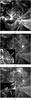 |
Fig. 3 171 Å images taken by TRACE. a) The arrow indicates the EUV channel corresponding to the filament involved in the eruption. b) Early phase of the eruption, when a highly twisted arcade becomes visible. The box shows a zoom on the western side of the arcade and the arrow indicates a crossing of type II. b) Main phase of the eruption. The box shows a zoom on the eastern side of the arcade and the arrow indicates a crossing of type III. The field of view is ~280 × 280 Mm2. North is at the top and west to the right. |
 |
Fig. 4 Value of the magnetic flux vs. time for the whole active region NOAA 9872. Continuous and dot-dashed lines indicate negative and positive flux, respectively. In this and in the following plots t = 0 corresponds to Oct. 28 at 23:59 UT and the vertical dashed line indicates the time when the filament eruption started. |
3. Results
In order to investigate the result further concerning the opposite magnetic helicity signs of the filament in Hα and the twisted arcade at 171 Å, we studied the horizontal velocity field and the magnetic helicity flux in the whole active region and over the regions where the filament footpoints were located before the eruption. Careful inspection of the velocity field in the photospheric regions characterized by magnetic discontinuities, i.e., where there is a mixture of polarities or polarity inversion lines, highlight the advantage of DAVE method with respect to the LCT method. We report in Figs. 5a and b the velocity fields on Oct 29 at 7:59 UT computed by the LCT and the DAVE methods, respectively. DAVE is able to detect the motion of the negative polarity inside the positive one near the inversion line, where the filament was located. These motions located in the regions where the gradient of B is significant are also visible from a visual inspection of the two sets of magnetograms. This pattern persists for all our observations until the negative polarity disappears.
As already stated, we used the velocity fields obtained by LCT and DAVE to compute of the magnetic helicity accumulation with the methods of Chae (2001) and Pariat et al. (2005). Figures 7a and b report the trend in the magnetic helicity accumulation over the whole active region during the two time intervals of observations. We can see that all the curves show a prevalent positive trend toward accumulating magnetic helicity in corona.
In particular, during the first time interval (Fig. 7a), the accumulation of magnetic helicity obtained with GA is always higher than with Gθ. This agrees with previous comparisons between GA and Gθ (Pariat et al. 2007). On the other hand, the accumulation obtained with the same method of helicity computation provided highest values when DAVE is used. This could be due to the already described ability of DAVE to detect the motion of the negative polarity inside the positive one near the inversion line where the filament was located. The accumulated helicity computed with different methods ranges from 4 to 11 × 1042 Mx2.
During the second time interval, the accumulation of magnetic helicity (Fig. 7b) is noticeably lower than the first time interval. From a visual inspection of the velocity fields, we do not note any particular variation in the average velocity strength. On the other hand, small episodes of flux cancellation are visible in the sequence of magnetograms. This could explain how the helicity flux becomes smaller in the second time interval in comparison to the previous one. It is worth noting that this behavior has been observed in several active regions by Jeong & Chae (2007), who show that usually the rate of helicity injection is initially low and that it increases and stays high for a while, and then becomes low again, while magnetic flux steadily increases at a more or less constant rate all the time. Moreover, two periods of weakly negative helicity transport rate are visible about 65 and 90 h after the beginning of our observations, respectively. The first period of negative rate was registered some hours after another flare of M3.2 occurred in the same active region at 8:09 UT on Oct. 31, while the second period corresponds to a few hours after the filament eruption we are considering in this paper (see Fig. 7b).
In the second time interval the accumulation of magnetic helicity obtained by LCT increases monotonically. This behavior can stem from the already mentioned minor capability of LCT to observe the displacement of the magnetic structures around the magnetic discontinuities. Therefore, the accumlation of the magnetic helicity obtained by LCT is dominated by the positive helicity flux above the main positive polarity characterized by a clockwise rotation, while the negative contribution coming from the inversion lines is underestimated in comparison to the helicity flux obtained by DAVE.
 |
Fig. 5 Map of the horizontal velocity field obtained by the LCT a) and DAVE b) methods overplotted on the magnetogram taken on Oct. 29 at 7:59 UT. The saturation levels are ±300 G. The field of view is ~280 × 280 Mm2. North is at the top and west to the right. |
 |
Fig. 6 Helicity density map obtained using the DAVE method for the velocity measures and the Pariat method for the helicity computation. The map corresponds to Oct. 29 at 20:47 UT. The field of view is ~280 × 280 Mm2 and is corrected for the projection effects by applying a standard differential rotation rate (Howard et al. 1990). North is at the top and west to the right. |
Comparison of the helicity maps obtained with both methods shows that Gθ removes many small-scale helicity density polarities observed in the GA maps, even though a global pattern remains: the leading magnetic region of positive polarity has positive helicity density, and the trailing region of negative polarity possesses negative helicity density (see Fig. 6). Such a pattern has already been observed and studied in detail in Pariat et al. (2007). The real helicity injected can be fully deduced only by the average of the flux at both polarities, provided that the connectivity is known (as we do for the filament hereafter).
Even though the total helicity flux computed with GA or Gθ should theoretically be strictly equal, the actual estimation on a discrete grid of a finite domain usually leads to some differences between these two proxies. For some flow pattern, GA can create spurious signal which can be an order of magnitude higher than with Gθ (Pariat et al. 2005). Even though the intense fake signals induced by GA computation should cancel, computation on a grid with a finite number of points naturally introduces errors that do not perfectly cancel when integrating the helicity flux. Because these errors are related to the intensity of the signal, Pariat et al. (2005), point out that GA misestimates the helicity flux more strongly than Gθ. When comparing the results obtained on real data, Pariat et al. (2006) recorded differences up to 15%, while Jeong & Chae (2007) report an active region for which the helicity injection rate determined with GA was about 30% higher than the rate obtained with Gθ.
In the present study the difference between GA and Gθ is relatively more than in previous studies. On average in the helicity maps, the value of GA is about 70% higher than the value of Gθ at the same location, while the maximum of GA is about 80% higher than the maximum of Gθ. This difference likely results from the fact that a relatively small amount of helicity is injected into AR 9682. While the accumulated helicity does not exceed ΔH = 1.1 × 1043 Mx2, the magnetic flux is φ ~ 4 × 10²² Mx, so that, for this active region the ratio ΔH/φ2 ≃ 0.008 is a few times smaller than the typical value found by Labonte et al. (2007) and Tian & Alexander (2008). The relative amount of helicity injected in this active region is thus relatively small given its magnetic flux. This agrees with the lack of major helicity carrying flows such as rotations. The consequence is that, since the helicity flux is relatively low, it is even more subject to errors in its estimation. As noted in Pariat et al. (2005) and Pariat et al. (2006), for a relatively smaller helicity flux, the discrepancy between GA and Gθ becomes larger. This active region is another illustration that GA should be avoided, even when computing the total helicity flux.
Considering the filament location in the Hα image at 10:55 UT (Fig. 2a), we determined the filament footpoints on the helicity density maps, and we could notice that all the maps obtained in our analysis show two persistent negative patches coincident with the filament footpoints. We named these patches corresponding to the eastern and western filament footpoints as A and B, respectively (see Figs. 6 and 2). In particular, it is worth noting that the shape of the patch A for most of the observing time recalls the negative magnetic intrusion we described before. Taking into account that the filament is formed by magnetic field lines filled by plasma and that the filament footpoints are anchored in the photosphere, we can consider the filament itself as a signature of the magnetic linkage of these patches. We nonetheless controlled the amount of magnetic flux unbalance in each of these patches. Balanced magnetic flux indeed implies that we considered a magnetic connectivity domain. During all our observations we never find a contrast, C, higher than 0.01, with C = (|φ+| − |φ−|)/(|φ+| + |φ−|) and with |φ±| the positive (negative) magnetic flux. Therefore, we guess that the magnetic helicity transported through these patches could provide most of the helicity accumulated along the field lines of the filament itself.
Figures 8a and b show the sum of the magnetic helicity accumulation in the patches A and B during the two MDI datasets. In this case we computed only Gθ because GA includes lots of weird cross helicity terms, and in these subfield-of-views, the comparison between the two methods should be meaningless. We observe that the negative helicity accumulated through the patches A and B is 4 orders of magnitude lower in absolute value than the net helicity accumulated in the whole active region and that more negative helicity is accumulated in the second dataset. We also notice that the DAVE method provided the highest values of magnetic helicity accumulation, even if both velocity methods show a similar trend in time.
 |
Fig. 7 a) and b) Magnetic helicity accumulation of the whole active region vs. time during the two datasets of MDI. |
 |
Fig. 8 a) and b) Magnetic helicity accumulation through the patches A and B of Fig. 6 vs. time during the two datasets of MDI. |
The negative injection in the negative magnetic polarity A can be understood as follows. The westward motion above the main positive magnetic polarity can be modeled as a clockwise rotation around the large positive polarity. Such motion does correspond to a negative magnetic helicity flux. In addition, above region A, a small positive polarity is also rotating around it clockwisely, which further increases the negative helicity injection. The motion of the patch B is mainly westward, with a small northern component. This motion away from the main positive polarity is not a helicity carrying one. However, the northern component constitutes a counterclockwise motion relative to the main negative polarity of the AR, hence a negative helicity injection. As actually observed, since the polarities are relatively far apart, the helicity injection in patch B is fainter than the helicity injection in patch A.
During the second time interval (Fig. 8b), the patches A and B are not persistent as in the first time interval and they appear more fragmented due to less coherent velocities above these regions. However, we still observe an helicity accumulation through all these patches of the same magnitude of the previous interval.
4. Discussion and conclusions
In this paper we studied a filament eruption in NOAA 9682 using Hα and 171 Å images, as well as MDI line-of-sight magnetograms. Analysis of 171 Å images showed that during the filament eruption a bundle of highly twisted threads were seen rising in the corona.
Although the morphology of the filament in the Hα images was ambiguous, calculating the magnetic helicity flux in the filament area and in the whole active region allowed us to deduce that the filament involved in the eruption showed a magnetic helicity flux at filament footpoints in accordance with negative magnetic helicity, while the overlying arcade and the environment field of the active region showed positive magnetic helicity. Another similar example of a filament carrying a local helicity of a different sign than the surrounding active region is presented in Chandra et al. (2010). Our results suggest that this filament eruption occurred in a region characterized by the interaction of two magnetic field systems with opposite signs of magnetic helicity.
We recall that, when positive and negative helicities coexist in a single domain, flux systems of opposite helicities can merge via reconnection leading to magnetic helicity cancellation. When this process occurs, the reconnected field may relax toward a state with lower total helicity, so there is less minimum energy, and the field energy corresponding to magnetic helicity of mixed signs can be released (Kusano et al. 2004). It is interesting, in this scenario, that the graph in Fig. 7b shows that the helicity accumulation in the whole active region calculated with the DAVE method is characterized by a significant decrease in the time period following the filament eruption. Therefore, it seems plausible to assume that the filament eruption, which is caused by reconnection between magnetic flux systems characterized by magnetic helicity of opposite sign, decreased the total helicity of the active region.
Moreover, as already pointed out in previous studies (Schuck 2005, 2006; Welsch et al. 2007; Chae & Sakurai 2008), the DAVE method has more accurately measured the horizontal velocities than the LCT method, especially near the magnetic inversion line where the filament was located. These more accurate measurements have strong effects on the magnetic helicity flux computation using both the method of Chae (2001) and the method of Pariat et al. (2005). Considering that the magnetic helicity is not a purely local quantity and that the motion of a given flux tube could inject mutual helicity into other flux tubes, i.e. in other regions, we find that the velocities detected by DAVE play a significant role not only in the local negative helicity injection through the region of the filament footpoints (Figs. 8a and b), but also in the positive helicity injection through the whole region. In fact, as suggested by the plots of Figs. 7a and b, these motions are also an effective source of mutual helicity.
Finally, although Gθ is a better proxy of the magnetic helicity flux density than GA, in our case the maps of both quantities showed a similar pattern, with negative patches at the filament footpoints and a dominant positive sign in the whole active region. However, a difference in the intensity of the helicity accumulation does appear.
Acknowledgments
The authors wish to thank Dr. Vasyl Yurchyshyn for providing the BBSO high-resolution images. This work was supported by the European Commission through the SOLAIRE Network (MTRN-CT-2006-035484), by the Instituto Nazionale di Astrofisica (INAF), by the Agenzia Spaziale Italiana (contract I/015/07/0), and by the Università degli Studi di Catania.
References
- Aulanier, G., & Demoulin, P. 1998, A&A, 329, 1125 [NASA ADS] [Google Scholar]
- Chae, J. 2000, ApJ, 540, L115 [NASA ADS] [CrossRef] [Google Scholar]
- Chae, J. 2001, ApJ, 560, L95 [NASA ADS] [CrossRef] [Google Scholar]
- Chae, J. 2007, Adv. Space Res., 39, 1700 [NASA ADS] [CrossRef] [Google Scholar]
- Chae, J., & Sakurai, T. 2008, ApJ, 689, 593 [NASA ADS] [CrossRef] [Google Scholar]
- Chandra, R., Pariat, E., Schmieder, B., Mandrini, C. H., & Uddin, W. 2010, Sol. Phys., 261, 127 [NASA ADS] [CrossRef] [Google Scholar]
- Démoulin, P. 2007, Adv. Space Res., 39, 1674 [Google Scholar]
- Démoulin, P., & Pariat, E. 2009, Adv. Space Res., 43, 1013 [NASA ADS] [CrossRef] [Google Scholar]
- Hartkorn, K., & Wang, H. 2004, Sol. Phys., 225, 311 [NASA ADS] [CrossRef] [Google Scholar]
- Howard, R. F., Harvey, J. W., & Forgach, S. 1990, Sol. Phys., 130, 295 [NASA ADS] [CrossRef] [Google Scholar]
- Jeong, H., & Chae, J. 2007, ApJ, 671, 1022 [NASA ADS] [CrossRef] [Google Scholar]
- Kusano, K., Maeshiro, T., Yokoyama, T., & Sakurai, T. 2004, ApJ, 610, 537 [NASA ADS] [CrossRef] [Google Scholar]
- LaBonte, B. J., Georgoulis, M. K., & Rust, D. M. 2007, ApJ, 671, 955 [CrossRef] [Google Scholar]
- Lin, J., Soon, W., & Baliunas, S. L. 2003, New Astron. Rev., 47, 53 [NASA ADS] [CrossRef] [Google Scholar]
- Meunier, N. 2004, A&A, 420, 333 [NASA ADS] [CrossRef] [EDP Sciences] [Google Scholar]
- Moon, Y. J., Chae, J. Y., Wang, H. M., Choe, G. S., & Park, Y. D. 2002, ApJ, 580, 528 [NASA ADS] [CrossRef] [Google Scholar]
- Nindos, A., Zhang, J., & Zhang, H. 2003, ApJ, 594, 1033 [NASA ADS] [CrossRef] [EDP Sciences] [Google Scholar]
- November, L. J., & Simon, G. W. 1988, ApJ, 333, 427 [Google Scholar]
- Pariat, E., Démoulin, P., & Berger, M. A. 2005, A&A, 439, 1191 [NASA ADS] [CrossRef] [EDP Sciences] [Google Scholar]
- Pariat, E., Nindos, A., Démoulin, P., & Berger, M. A. 2006, A&A, 452, 623 [NASA ADS] [CrossRef] [EDP Sciences] [Google Scholar]
- Pariat, E., Démoulin, P., & Nindos, A. 2007, Adv. Space Res., 39, 1706 [NASA ADS] [CrossRef] [Google Scholar]
- Romano, P., Contarino, L., & Zuccarello, F. 2005, A&A, 433, 683 [NASA ADS] [CrossRef] [EDP Sciences] [Google Scholar]
- Schrijver, C. J. 2009, Adv. Space Res., 43, 739 [NASA ADS] [CrossRef] [Google Scholar]
- Schuck, P. W. 2005, ApJ, 632, L53 [NASA ADS] [CrossRef] [Google Scholar]
- Smyrli, A., Zuccarello, F., Romano, P., et al. 2010, A&A, 521, A56 [NASA ADS] [CrossRef] [EDP Sciences] [Google Scholar]
- Tian, L., & Alexander, D. 2008, ApJ, 673, 532 [NASA ADS] [CrossRef] [Google Scholar]
- Welsch, B. T., Abbett, W. P., De Rosa, M. L., et al. 2007, ApJ, 670, L1434 [NASA ADS] [CrossRef] [Google Scholar]
- Zhang, Y., Tan, B., & Yan, Y. 2008, ApJ, 682, L133 [NASA ADS] [CrossRef] [Google Scholar]
All Figures
|
Fig. 1 Hα image of NOAA 9682 acquired by the 66.05 cm telescope at Big Bear Solar Observatory on Oct. 31 at 23:20 UT. The white arrow indicates the barb of the filament involved in the eruption. The field of view is ~390 × 390 Mm2. North is at the top and west to the right. |
| In the text | |
|
Fig. 2 a) Hα image of NOAA 9682 acquired at INAF-Catania Astrophysical Observatory on Nov. 1 at 10:55 UT. The white arrow indicates the filament involved in the eruption. b) Line-of-sight magnetogram taken by MDI on Nov. 1 at 11:11 UT. The saturation levels are ±300 G. The black line indicates the filament location. The contours A and B correspond to the negative patches of the helicity density at filament footpoints (see also Fig. 6). The field of view is ~280 × 280 Mm2 and is corrected for the projection effects by applying a standard differential rotation rate (Howard et al. 1990). North is at the top and west to the right. |
| In the text | |
|
Fig. 3 171 Å images taken by TRACE. a) The arrow indicates the EUV channel corresponding to the filament involved in the eruption. b) Early phase of the eruption, when a highly twisted arcade becomes visible. The box shows a zoom on the western side of the arcade and the arrow indicates a crossing of type II. b) Main phase of the eruption. The box shows a zoom on the eastern side of the arcade and the arrow indicates a crossing of type III. The field of view is ~280 × 280 Mm2. North is at the top and west to the right. |
| In the text | |
|
Fig. 4 Value of the magnetic flux vs. time for the whole active region NOAA 9872. Continuous and dot-dashed lines indicate negative and positive flux, respectively. In this and in the following plots t = 0 corresponds to Oct. 28 at 23:59 UT and the vertical dashed line indicates the time when the filament eruption started. |
| In the text | |
|
Fig. 5 Map of the horizontal velocity field obtained by the LCT a) and DAVE b) methods overplotted on the magnetogram taken on Oct. 29 at 7:59 UT. The saturation levels are ±300 G. The field of view is ~280 × 280 Mm2. North is at the top and west to the right. |
| In the text | |
|
Fig. 6 Helicity density map obtained using the DAVE method for the velocity measures and the Pariat method for the helicity computation. The map corresponds to Oct. 29 at 20:47 UT. The field of view is ~280 × 280 Mm2 and is corrected for the projection effects by applying a standard differential rotation rate (Howard et al. 1990). North is at the top and west to the right. |
| In the text | |
|
Fig. 7 a) and b) Magnetic helicity accumulation of the whole active region vs. time during the two datasets of MDI. |
| In the text | |
|
Fig. 8 a) and b) Magnetic helicity accumulation through the patches A and B of Fig. 6 vs. time during the two datasets of MDI. |
| In the text | |
Current usage metrics show cumulative count of Article Views (full-text article views including HTML views, PDF and ePub downloads, according to the available data) and Abstracts Views on Vision4Press platform.
Data correspond to usage on the plateform after 2015. The current usage metrics is available 48-96 hours after online publication and is updated daily on week days.
Initial download of the metrics may take a while.