| Issue |
A&A
Volume 525, January 2011
|
|
|---|---|---|
| Article Number | A127 | |
| Number of page(s) | 17 | |
| Section | Extragalactic astronomy | |
| DOI | https://doi.org/10.1051/0004-6361/200811129 | |
| Published online | 08 December 2010 | |
The dependence of X-ray AGN activity on host galaxy properties and environment⋆
1
GEPI, Observatoire de Paris-Meudon, 5 place Jules Janssen, 92190
Meudon, France
e-mail: This email address is being protected from spambots. You need JavaScript enabled to view it.
2
Leiden Observatory, University of Leiden,
PO Box 9513, 2300 RA
Leiden, The
Netherlands
3
SUPA, Institute for Astronomy, Royal Observatory
Edinburgh, Blackford
Hill, Edinburgh
EH9 3HJ,
UK
Received:
10
October
2008
Accepted:
16
June
2010
Abstract
There is mounting evidence that active galactic nuclei (AGN) selected through optical emission lines or radio luminosities comprise two distinct AGN populations, whose activity is triggered by different processes. In two previous papers, we studied the host galaxies and environment of radio-loud AGN. In this third paper we study the properties of a sample of Type-2 AGN that were selected on the basis of their [2–10] keV X-ray luminosity. We find that the X-ray luminosity function is in good agreement with previous studies and that the fraction of galaxies hosting an X-ray AGN is a strong function of the stellar mass of the host galaxy. The shape of this fraction-mass relation is similar to the fraction of galaxies that are emission-line AGN, while it differs significantly from the relation observed for radio-selected AGN. The AGN in our sample tend to be located in underdense environments where galaxy mergers and interactions are likely to occur. For all host galaxy masses, the Type-2 AGN display a strong infrared excess at short (~3.5 μm) wavelengths, suggesting the presence of hot dust possibly associated with a hot dusty torus. These results add weight to the belief that the X-ray selection criteria identifies a population of AGN similar to the emission-line selected population but distinct from the radio population at high masses.
Key words: galaxies: active / galaxies: fundamental parameters / quasars: emission lines / X-rays: galaxies / large-scale structure of Universe
Appendix A is only available in electronic form at http://www.aanda.org
© ESO, 2010
1. Introduction
It is becoming increasingly clear that active galactic nuclei (AGN) play an important role in the framework of galaxy formation. The enormous amounts of energy produced by AGN during their short lifetimes can dramatically influence the evolution of both their host galaxies and their surrounding environment (e.g. Croton et al. 2006; Springel et al. 2005).
Although AGN have been studied for decades, many aspects of their physics remain poorly understood. In the unified scheme of AGN, energy is produced by the accretion of matter onto a super-massive black hole, which is surrounded by a dusty torus. This simple scheme can explain many properties of the different classes of AGN in different wavelength bands. However, observational evidence is mounting to suggest that this picture does not give a proper description for low-luminosity radio-loud AGN (P1.4 GHz ≲ 1025 W Hz-1). These objects produce weaker or no emission lines (Hine & Longair 1979; Jackson & Rawlings 1997), lack the dusty torus infrared emission (Ogle et al. 2006), and do not produce the accretion related X-ray emission (Hardcastle et al. 2006). It has been suggested that there are indeed two very different modes of AGN activity named the “Quasar mode” and the “Radio mode” (Best et al. 2005; Hardcastle et al. 2007). A physical interpretation has been proposed in which the infall of cold gas onto the super-massive black hole gives rise to the radiatively efficient quasar mode, while the hot gas infall produces the radiatively inefficient radio mode (Hardcastle et al. 2007).
The undertaking of large surveys provides the opportunity to study the nature of the AGN activity (see Heckman & Kauffmann 2006, for a review of the SDSS results). Based on a sample of radio-selected AGN in the Canada France Hawaii Telescope Legacy Survey (CFHTLS) field (Tasse et al. 2008b), we have argued in favour of a dichotomy in the properties of the population with stellar mass with a separation at Mcut ~ 1010.5−10.8 M⊙ (Tasse et al. 2008a). The high stellar mass systems were mainly found in denser environments than normal galaxies of the same stellar masses (on the ~500 kpc scale), while they did not show any signs of hot dust emission in the infrared. The properties of the lower stellar mass systems were quite different: they displayed a hot dust component and lay in 500 kpc scale underdensities (as compared to normal galaxies of the same stellar mass). This result suggests a direct link between the density of the large-scale environment and the properties of the matter in the inner 10−100 pc regions of galaxies. We have argued (Tasse et al. 2008a) that these radio-selected AGN trace very different populations, with the AGN activity of the low-mass population triggered by galaxy mergers and interactions, while the high-mass systems have their AGN activity triggered by the gas cooling in their hot atmosphere (Best et al. 2005, 2006). Based on the hot infrared excess that is only observed in the low-mass systems, we argued that these observations are consistent with the picture discussed by Hardcastle et al. (2007), where the hot gas cooling produces radiatively inefficient accretion (radio mode), and the cold gas accretion, perhaps triggered by galaxy mergers and interactions, drives radiatively efficient accretion (quasar mode).
A good way to further test the scheme in which the type of the accretion mode is connected to the nature of the triggering mechanism, is to select AGN based on their X-ray properties. In the unified scheme, the hard X-ray emission is produced in the hot corona that surrounds the black hole, by the Comptonisation of soft UV photons which are emitted by the accretion disk (e.g. Liu et al. 2002). In this paper we present a similar study to that of Tasse et al. (2008a), using a sample of hard X-ray selected ([2–10] keV band) Type-2 AGN (i.e. those without a bright optical quasar component) instead of a sample of AGN selected based on their radio luminosity. By using the photometric redshifts, stellar masses, and overdensity estimates (Tasse et al. 2008a), we study the internal and environmental properties of the host galaxies of the X-ray selected AGN in an independent manner. Our results suggest that, unlike the radio population, at all stellar masses the X-ray selected Type-2 AGN population is dominated by AGN in their quasar mode, which are triggered by galaxy mergers and interactions (cold gas).
In Sect. 2 we briefly review the infrared, optical and X-ray data available for the XMM-LSS field. In Sect. 3, we proceed with the optical identification, and we select a subsample of Type-2 sources for which we derive physical parameter estimates. We present the results in Sect. 4, and discuss them in Sect. 5.
2. Multiwavelength dataset
2.1. XMM-LSS X-ray survey
The XMM-Large Scale Structure field (XMM-LSS) is a wide ~10 deg2 extragalactic window situated at high galactic latitudes which was surveyed by the XMM-Newton satellite in the [0.5–10] keV energy band. Figure 1 shows the location of the XMM-Newton pointings with respect to the SWIRE infrared survey (Spitzer Wide-area InfraRed Extragalactic legacy survey, Lonsdale et al. 2003), CFHTLS-W1 optical survey (Canada France Hawaii Telescope Legacy Survey – Wide1), and low-frequency radio surveys (Tasse et al. 2006, 2007). Galaxy clusters are detected as extended X-ray emission, and X-ray emitting AGN are detected as point-like sources. Their surface number densities reach ~12 and ~200 deg-2, respectively (see Pierre et al. 2004, for a layout of the XMM-LSS and associated surveys).
In this paper we consider the X-ray catalogue described in great detail in Pacaud et al. (2006). The catalogue was built from the raw X-ray data in three steps: (i) solar proton flares are removed; (ii) the X-ray images are filtered using wavelets; and (iii) using a maximum likelihood procedure, the profiles of detected sources are fitted to determine whether they are point-like or extended. This pipeline has been characterised in great detail using extensive Monte-Carlo simulations (Pacaud et al. 2006). The final band-merged catalogue contains sources detected in the [0.5–2] and [2–10] keV bands respectively, referred to as “soft” and “hard” bands.
The absorption of X-ray photons in general produces a strong decline of the emitted luminosity in the soft X-ray bands (e.g. Reynolds 1997), while this effect is less important at higher energies. Therefore, for our purposes we select those X-ray sources in the [2–10] keV hard band that (i) have been classified as point-like and that (ii) have a likelihood ratio of detection LRDETsuch that LRDET > 15(see Pacaud et al. 2006, for a detailed description of LRDET). The flux in the two available bands was computed from the photon count rates assuming a single power law spectrum Fν ∝ ν-0.8and the average galactic column density of the XMM-LSS field: NH = 2.61 × 1020 cm-2(Dickey & Lockman 1990).
In order to proceed with the optical identification we have selected X-ray sources overlapping with the CFHTLS-W1 field (Sect. 2.2). The final X-ray sample contains 1001 sources. Following Chiappetti et al. (2005), we assume that the error on the position of X-ray sources is σα,δ = 3″.
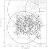 |
Fig. 1 The location of the CFHTLS, SWIRE, XMM-LSS fields. The black dots show the X-ray sources selected for optical and infrared identification. |
2.2. Optical and infrared surveys
The XMM-LSS field is partially covered by the Wide-1 component of the CFHTLS. Observations were conducted using the five u∗g′r′i′z′ broad band optical filters, with typical exposures of 1 h in each filter. The i-band limiting magnitude is i ~ 24.5(80%completeness level), with positional uncertainties of ~0.3″. In this paper we have used the band merged catalogues Terapix T02 and T03 releases2, that overlap the X-ray field over ~3.7 deg2.
The Spitzer Wide-area InfraRed Extragalactic legacy survey (SWIRE, Lonsdale et al. 2003) covers the XMM-LSS field over 9.1 deg2, using the IRAC instrument from 3.6to 8.0 μm and MIPS from 24to 160 μm (See Fig. 1). Throughout this paper we have used the data release 2 (DR2 hereafter) band merged catalogue, available online3, containing the flux density measurements at 3.6, 4.5, 5.8, 8.0and 24 μm for a total of ~2.5 × 10⁵ objects. This catalogue contains sources detected at 5σfrom the 3.6to 8.0 μm images and at 3σfrom the 24 μm images, corresponding to sensitivity limits of 14, 15, 42, 56, and 280 μJy, respectively, with positional accuracies better than 0.5″(2σ). The data reduction and quality assessment is extensively discussed in Surace et al. (2004).
3. A sample of X-ray selected Type-2 AGN
3.1. Optical identification
In this section we identify optical counterparts for the 1001 point-like X-ray sources of the sample described in Sect. 2, and using the SWIRE infrared data, we associate infrared flux density measurements to these optical objects.
We quantify the probability of an i′-band optical object being the true host of a given X-ray point-like source by using a modified version of the likelihood ratio method, first described by Richter (1975) and subsequently modified by de Ruiter et al. (1977), Prestage & Peacock (1983), Benn (1983), Wolstencroft et al. (1986) and Sutherland & Saunders (1992). The Sutherland & Saunders (1992) version of the likelihood ratio technique used here allows us to derive, for each X-ray point-like source, a probability of association with any optical object that potentially takes into account its position offset, magnitude, colour, etc. This is done under the assumption the X-ray point-like emission is produced at the physical location of optical emission (detected or not). As shown in Tasse et al. (2008b), quantifying the individual probabilities of association rather than than simply doing a one-to-one association with an overall reliability level, allows us to probe the AGN activity of a low stellar mass galaxy population and to reach a good understanding of the different contamination effects. All numbers derived in the next sections are calculated from the sum of those association probabilities for a given subset of X-ray sources4. This version of the likelihood ratio method is discussed in great detail in Tasse et al. (2008b), but for completeness we briefly discuss the technique here.
The likelihood ratio is defined as the probability that the X-ray source has its true optical candidate detected and lying at a certain angular distance, divided by the probability that the given optical candidate is a background or foreground source. The probability that a given source is the true optical counterpart is then calculated as a function of the estimated likelihood ratio of all possible counterparts using the formulae of Sutherland & Saunders (1992). The likelihood ratios, as well as the association probability estimates, depend on the individual positional error bars, but also on both the distribution of X-ray sources hosts and background sources in the parameter space for the ~2 × 10⁶ galaxies detected in the CFHTLS optical data (i-band magnitude i, photometric redshifts z, specific star formation rates sSFR, and stellar masses M as estimated by Tasse et al. 2008b, see Sect. 3.2). Although the distribution of X-ray sources hosts in the parameter space is unknown, that of the background sources can be easily estimated. By using extensive Monte-Carlo simulations we have recursively constrained the contribution of background sources in the derived distribution of X-ray sources hosts in the parameter space as follows.
First, the likelihood ratio is estimated only using the a priori probability θ(m)that an X-ray counterpart has a magnitude <m (see Fig. 2). This information is derived by comparing the distribution of the distance dminbetween the X-ray sources and their closest optical object to the same distribution for a simulated catalogue in which a variable fraction of X-ray sources have an optical counterpart (see Tasse et al. 2008b, for the details). We find that ~76%of the X-ray sources have an optical counterpart at the limiting magnitude of the i-band optical data.
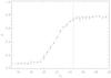 |
Fig. 2 In order to identify the optical counterparts of X-ray AGN, we take into account the magnitude distribution of X-ray sources hosts, which is different from that of the confusing background sources. The estimated fraction (y-axis) of X-ray AGN having an optical counterpart with i-band below magnitude m(x-axis), has been determined using a Monte-Carlo simulation (see Tasse et al. 2008b, for the details). Around 76%of X-ray sources have an optical counterpart at the limiting magnitude of our survey (the vertical dotted line shows the 80% completeness level of the optical survey). |
However, it appears that only taking into account the information on magnitude, drives a contamination effect by background sources when inspecting the properties of X-ray sources hosts for parameters other than the magnitude (such as stellar mass, star formation rate, or photometric redshift, see Tasse et al. 2008b). The second step corrects for this effect, by generating a random catalogue in which a fraction θ(m)of X-ray sources have an optical counterpart with a magnitude <m. The association probabilities are then calculated in the same manner (using θ(m)only) and knowing the true optical counterpart, the contribution of background sources to those probabilities is estimated. The distribution θ(m,M,sSFR,z)of X-ray sources hosts in the parameter space is then corrected for the contribution of background sources and re-normalised. We used θ(m,M,sSFR,z)to derive the final association probability. For each X-ray source we obtain a probability of association with its 5 closest optical objects. Of the 1001 point-like X-ray sources, 769 have a detected optical counterpart5.
To associate counterparts in the infrared SWIRE images with the X-ray sources, we follow Surace et al. (2004), and require them to be closer than 1.5″. The source density in the SWIRE DR2 band merged catalogue is ~3.2 × 10⁴ deg-2. Assuming Poisson statistics, the chance of association with a random background source is ~2%. Of the sources associated with an optical counterpart in the CFHTLS data, 78%are also associated with an infrared source as detected by IRAC.
3.2. Spectral energy distribution fitting and sample selection
In this section we follow in detail the method of Tasse et al. (2008b) to select a sample of Type-2 AGN for which photometric redshifts and stellar masses are reliable. This method is based on both SED fitting and colour-colour selection.
In Tasse et al. (2008b) we fit the u∗g′r′i′z′ and IRAC flux density measurements with spectral energy distribution (SED) templates for the ~2 × 10⁶galaxies detected in the CFHTLS optical data. Following Tasse et al. (2008b), we have removed the faint sources and bright saturated objects (18 < i < 24; selection criteria “SC1” hereafter), and the sources overlapping the masked areas in the i-band optical images (SC2). In addition, since the 4000 Å break is the most constraining feature of the optical spectrum, we limit our study to the redshift range 0.1 < z < 1.2(SC3), where the upper limit corresponds to the 4000 Å break redshifting into the z′-band filter (Tasse et al. 2008b).
In order to estimate the photometric redshifts we have used two complementary SED fitting methods. The first method uses ZPEG, whose SED template library was built from the stellar synthesis model of Le Borgne & Rocca-Volmerange (2002). For each of the best fitting templates, ZPEG returns estimates for the redshift, stellar mass, and specific star formation rate (sSFR0.5 hereafter). Because the stellar synthesis model does not take into account the dust emission, which can dominated the infrared fluxes, we have used only the u∗g′r′i′z′ magnitude measurements to constrain the SED fitting. The second approach uses the SWIRE template library of Polletta et al. (2006), which was built from both observations and theoretical modelling. This library contains both normal galaxy templates and optically active AGN templates such as QSO type 1. The combination of these two methods allows us to (i) obtain a good understanding of the overall content of our sample and (ii) reject the objects for which the ZPEG output parameters are unreliable.
As discussed in Tasse et al. (2008b) the host galaxies of optically active Type-1 AGN, may have their SED dominated by the AGN light. Therefore, in order to study the properties of AGN using photometric redshifts, stellar masses, and sSFR0.5 as estimated by ZPEG, we need to detect and remove the Type-1 AGN, for which the photometric redshift are not reliable. To do this, we follow the method of Tasse et al. (2008b) who discussed in detail the criteria used to select Type-2 radio source host galaxies. This selection is based on a combination of criteria: (i) the stellaricity parameter derived from the i-band optical images (selection criteria “SC4”); (ii) the g′ − r′versus r′ − i′colour–colour diagram (SC5); and (iii) the result of the SED fitting procedure using the SWIRE templates library (SC6, containing Type-1 AGN templates, see Tasse et al. 2008b, for details). The X-ray selected AGN classified as Type-1 using the criteria (iii) are represented by open circles in Fig. 3. Of the 253 selected optical counterparts that not been flagged after the SC1, SC2 and SC3 selection criteria discussed above, 190 have been classified as Type-2 AGN by the SC4, SC5, and SC6 selection criteria. This sample is presented in Table A.1. For clarity, this table includes only the optical candidates that have a probability of association with a given X-ray source greater than 1%.
The top panel of Fig. 3 shows the location of all the optical counterparts6 of the X-ray and radio AGN (Tasse et al. 2008b) in a g′ − r′versus r′ − i′colour–colour diagram7. The dashed area indicates the selection criteria that have been used to classify the sources as Type-1 using SC5 (based on optical colours; open diamonds), whereas the open circles show the sources classified as contaminating Type-1, using SC6 based on the spectral fits as described in Tasse et al. (2008b). Clearly, X-ray selected AGN optical counterparts show differences from the optical hosts of radio-loud AGN. The majority of the X-ray selected AGN (~40%) lie inside the Type-1 area, versus a ~12%fraction for the radio-loud AGN. A significant fraction of X-ray AGN that are located outside that area are classified as contaminating (~7%) by the spectral fit criteria (Tasse et al. 2008b).
The bottom panel of Fig. 3 shows the [3.6]–[4.5] versus [5.8]–[8.0] infrared colour-colour plot for all the infrared counterparts6of X-ray sources having flux density measurement in all IRAC bands. Stern et al. (2005) argues that 90%of the broad-line AGN lie within the area indicated by the dotted lines, as well as ~40% of the narrow-line AGN, and 7%of normal galaxies. We find that ~90%of the sources calssified as Type-1 AGN lie within this region in agreement with the estimate of Stern et al. (2005). Consistently, this fraction goes down to ~60%for the sources classified as Type-2, in contrast with the ~20%found for the radio-selected AGN (Tasse et al. 2008b).
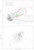 |
Fig. 3 Top panel: the g′ − r′versus r′ − i′ colour–colour diagram for all the optical counterparts of X-ray sources (black dots, applying selection criteria SC1 and SC2 only6). Open circles indicate the optical counterparts of X-ray sources that have been classified as Type-1 AGN by the spectral fit criteria using the IRAC bands (SC6). The dashed area indicates the region corresponding to the optical g′ − r′versus r′ − i′ selection criteria used to reject the contaminating Type-1 AGN (SC5, grey diamonds). Radio source host galaxies (indicated by crosses) and X-ray optical counterparts clearly occupy different regions of this plot, with the radio-loud AGN more typically hosted by galaxies that do not show strong signs of AGN activity in the optical. We also plot the colour-colour tracks for a Type-1 QSO, an elliptical, and a starburst galaxy. The square, star, diamond and triangle symbols stand for redshifts 0, 0.5, 1.5, and 2 respectively. Bottom panel: the [3.6]–[4.5] versus [5.8]–[8.0] infrared colour–colour diagram. Stern et al. (2005) find ~90%of the broad-line AGN lying in the area delimited by the dotted line. Symbols are as in the top panel. The sources marked as open circles and diamonds have been rejected from our sample. |
3.3. Extinction correction
In this section we estimate the hydrogen column density of the obscuring material for each of the individual sources, and derive their intrinsic luminosities.
The X-ray spectra of Type-2 AGN can show strong absorption at low energies, due to the presence of obscuring material in the line of sight (see Sect. 2.1). Following Tajer et al. (2007), we define the hardness ratio as HR = (CRH − CRS)/(CRH + CRS), where CRHand CRSare the count rates in the hard [2–10] and soft [0.5–2] keV band, respectively. Figure 4 shows the distribution of HRfor the sources selected as Type-1 and Type-2 as described above. As expected, these results indicate that the selected Type-2 AGN have a higher hardness ratios than the Type-1 AGN population, due to their higher column densities (Tajer et al. 2007).
Sazonov & Revnivtsev (2004) have estimated column densities from the flux ratio F [8−20] /F [3−8] , where F [8−20] and F [3−8] are the flux measurements in the [8–20] and [3–8] keV X-ray bands respectively. They have shown that these estimates are good first-order approximations of the estimates derived from fitting the X-ray spectra with an absorption model. Using the X-ray pipeline XSPEC, we follow a similar approach. We assume an X-ray AGN spectrum Fν ∝ ν-0.8at a redshift z, absorbed with an equivalent hydrogen column density of nH(model named “zphabs*pow” in XSPEC). From this model, we compute the observed ratio F [0.5−2] /F [2−10] in the { z,nH } parameter space, where F [0.5−2] and F [2−10] are the fluxes measured in the soft and hard X-ray band respectively (Sect. 2.1).
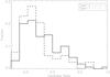 |
Fig. 4 Hardness ratio distribution for the sources that have been selected (Type-2) and rejected (Type-1). As is expected, the sources showing signs of absorption in the optical and infrared domains have higher hardness ratios. |
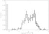 |
Fig. 5 Based on the observed flux ratio F [0.5−2] /F [2−10] , assuming an underlying Fν ∝ ν-0.8X-ray spectra, we have estimated the hydrogen column density for the sample of Type-2 AGN selected in Sect. 3.2. The shaded region shows the fraction of sources in our sample that have hydrogen column density lower than 1020 cm-2. As expected, most of the AGN we have selected show signs of absorption in their X-ray spectra. |
Figure 5 shows the estimated column density for the sample of optically selected Type-2 AGN (Sect. 3.2). Tajer et al. (2007) have derived the column densities for optically selected Type-1 and Type-2 sources, by fitting the X-ray spectra with a photo-absorption model. In their sample of ~130 X-ray AGN they find that for the objects selected as obscured by optical criteria, 63 ± 18%and 36 ± 12%have nH > 1021and nH > 1022 cm-2, respectively, while only ~20%of the objects classified as unobscured have nH > 1021 cm-2. In our selected Type-2 sample, we find that 64 ± 7%and 38 ± 5%have nH > 1021and nH > 1022 cm-2, respectively. These estimates are in good agreement, even though we are using a simple approach to estimate nH. However, we point out we only have a few detections of X-ray AGN with nH > 1023 cm-2, while those are known to be numerous at low redshift at least (at levels of ~75% Risaliti et al. 1999). This aspect is further discussed in Sect. 4.3.
We have used the estimates of the hydrogen column density nHto convert the observed luminosities to intrinsic luminosities. We note that our method to derive column densities is simplistic, and the combined uncertainties on the X-ray fluxes, redshifts, and assumed spectral index have to be taken into account to estimate the final errors on the column density and hence on the intrinsic luminosity estimates. In order to estimate those errors, we have run a Monte Carlo simulation for 100 X-ray spectra taking into account the distribution of the individual input parameters. For each X-ray spectra, we quantify the difference between the true underlying luminosity and hydrogen column density (Ltrue,nH,true) and the measured ones (Lmes,nH,mes). This analysis shows that the 50, 70and 90%quantiles of the dlog (nH) ≡ log 10(| nH,mes − nH,true | )distribution are q50 ~ −0.33, q70 ~ 0.47and q90 ~ 1.4. For the dlog (L) ≡ log 10(| Lmes − Ltrue | /Ltrue) distribution we find q50 ~ −0.62, q70 ~ −0.41and q90 ~ −0.04, which corresponds to errors on the estimated absorption-corrected X-ray luminosity better than 22, 39, and 85%for 50, 70and 90%of the sample.
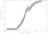 |
Fig. 6 The cumulative distribution of the difference between our estimate of the photometric redshift and the spectroscopic redshift as measured by Stalin et al. (2010). The dashed line shows a normal distribution with σ(Δz) = 0.1. |
4. Properties of Type-2 X-ray selected AGN
4.1. Redshift estimates
Stalin et al. (2010) have obtained spectra for a sample of 487 X-ray sources in the XMM-LSS field. In order to test the reliability of our photometric redshifts, we have compared the spectroscopic and photometric redshift estimates for the 39 cross-identified optical hosts classified as being associated with a Type-2 X-ray AGN (see Fig. 6). The distribution of the difference Δzbetween the two redshift estimates is a good fit to a Gaussian distribution having a standard deviation of σ(Δz) = 0.1, in agreement with the σ(Δz) = 0.09expected by Tasse et al. (2008b).
4.2. Luminosity function
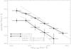 |
Fig. 7 We have estimated the X-ray luminosity function in the 0.1 < z < 0.5and 0.5 < z < 1.0redshift bins. Our estimates are in good agreement with the results presented in Steffen et al. (2003). |
As a further test of the consistency of the photometric redshifts and X-ray luminosities estimates for our selected sample of X-ray AGN, we derive an X-ray luminosity function and compare it to previous results.
We compute comoving number density estimates by using the 1/Vmaxestimator (Schmidt 1968), where Vmaxis the maximum volume over which a given object is observable. To do this we first estimate the dependence of the effective area on the X-ray flux, following Steffen et al. (2003), by simply comparing our source count at each flux to the source counts given by Cowie et al. (2002). For each given X-ray source we then use XSPEC, as well as the estimated luminosity and column density, to obtain the flux at each redshift, as well as the corresponding effective area. We obtain Vmaxby integrating between zminand zmaxthe probed volume element at each redshift. We have estimated zminand zmaxfor the optical data using the best fit ZPEG SED (see Tasse et al. 2008a, for details). Figure 7 shows the X-ray luminosity function computed using the 1/Vmaxestimator in the 0.1 < z < 0.5and 0.5 < z < 1.2redshift ranges.
Based on a sample of ~150 sources having spectroscopic redshifts, Steffen et al. (2003) have computed the X-ray luminosity function for the ranges 0.1 < z < 0.5and 0.5 < z < 1.0 in the [2–8] keV band. In order to compare our results with theirs, we assume X-ray spectra with Fν ∝ ν-0.8, and derive an L [2−8] − L [2−10] conversion factor. Our estimates are in broad agreement with Steffen et al. (2003) for both the high and the low-redshift ranges. The observed difference might be explained by the selection criteria used to define the AGN samples: the luminosity function as estimated by Steffen et al. (2003) was drawn from samples of both Type-1 and Type-2 objects, while we have selected a sample of Type-2 AGN.
Given that we have classified 63 galaxies as being Type-1 AGN and 190 as being Type-2 AGN (in the 0.1 < z < 1.2, 18 < i < 24selected sample, see Sect. 3.2), the difference in comoving density would correspond to ~0.1 dex if the Type-1 and Type-2 AGN were similarly distributed; this is quite consistent with the mean offset observed. Nevertheless, the slope of our estimate of the X-ray luminosity function seems to be quite different from the one presented in Steffen et al. (2003), especially in the higher redshift bin. Those differences are understandable because: (i) the populations of Type-1 and Type-2 AGN are known to evolve differently; (ii) the comparison is done under the assumption that all X-ray sources have an X-ray spectra with Fν ∝ ν-0.8and (iii) significant uncertainties are associated with our estimates of the intrinsic X-ray luminosities (Sect. 3.3). However, the overall good agreement between the two estimates of the X-ray luminosity function suggests that the physical parameters of the host galaxies of Type-2 X-ray AGN as derived using photometric redshifts are valid on average. Those results are further discussed in Sect. 5.
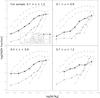 |
Fig. 8 The fraction of galaxies that are X-ray AGN with L [2−10] > 1043 erg s-1, as a function of the stellar mass, in the 0.1 < z < 1.2, 0.1 < z < 0.6, 0.4 < z < 0.9and 0.7 < z < 1.2redshift ranges. At low redshift the slope of the relationship shows good agreement with the fraction of galaxies that are classified as AGN based on emission-line criteria (Best et al. 2005), while it seems to evolve in the same way as the radio-loud fraction of galaxies at low stellar masses. |
4.3. Fraction-mass relations
Using the number density estimator described in Sect. 4.2, we have computed the mass function (φX) for the host galaxies of X-ray AGN and the fraction fXof galaxies that are X-ray AGN above a certain X-ray luminosity. This is simply computed as fX = φX/φOpt, where φOptis our estimate of the mass function for normal galaxies (see Tasse et al. 2008b). Figure 8 shows the estimates of fXfor the redshift ranges 0.1 < z < 1.2, 0.1 < z < 0.6, 0.4 < z < 0.9and 0.7 < z < 1.2and for X-ray luminosities LX > 1043 erg s-1.
For comparison, we have plotted the equivalent relation for the low-redshift (z ≲ 0.3) emission-line selected AGN with luminosities LO [III] > 106.5 L⊙ and LO [III] > 107.5 L⊙, and radio-selected AGN with 1.4 GHz radio luminosities P1.4 > 1024 W Hz-1 (Best et al. 2005; Tasse et al. 2008b) and P1.4 > 1025 W Hz-1 (Best et al. 2005). Interestingly, in the lowest redshift bin, the shape of the fraction-mass relation (fX ∝ M ~ 1.5) of the X-ray selected AGN resembles that of the emission-line AGN. Furthermore, the slope of this relation shows good agreement with that of the radio selected AGN of low stellar mass (M ≲ 1010.5−11 M⊙). In the higher redshift bins the relation seems to flatten. This suggests that the AGN activity of the massive galaxies evolves less than that of the lower stellar mass galaxies over 0.1 < z < 1.2.
Following Tasse et al. (2008a), we investigate whether the uncertainties on stellar mass estimates (Δ(log 10(M/M⊙)) ~ 0.4, see Tasse et al. 2008b) could give rise to the flattening of the slope in the higher redshift bins. To do this we generate random X-ray AGN samples characterised by a variable fraction-mass relation fX = C11Mα, where C11is the normalisation of the power law at 1011 M⊙, and αis the slope of the fraction-mass relation. We associate to each of those objects a random stellar mass with a probability distribution estimated from the original catalogue. Considering the measured estimates and their associated error bars, we derive a χ2in the C11 − αparameter space to obtain a best fit value and the associated uncertainties. Figure 9 shows that the values of C11and αfor the best fit are still consistent with a slope of α ~ 1.7at low redshift, and a flattening of the fX − M relation in the higher redshift bins. This mass-dependent evolution is further discussed in Sect. 4.4 by studying the V/Vmaxstatistics.
In order to directly compare our X-ray luminosities with emission-line luminosities, we use the L [3−20] versus LO [III] relation given by Heckman et al. (2005) in the [3–20] keV band (log (L [3−20] /LO [III] ) = 2.15), with a conversion factor between the [3–20] and [2–10] keV bands (assuming an X-ray spectra with Fν ∝ ν-0.8). The LX > 1043 erg s-1 X-ray luminosity corresponds to [OIII] line luminosities of LO [III] > 107.5 L⊙. In the lower redshift bin the difference between those two populations is as high as ~0.7−1.2 dex. Differences are to be expected: Heckman et al. (2005) have shown that X-ray selection criteria miss a significant fraction of emission-line AGN. Specifically, at z ≲ 0.1the normalisation of the AGN luminosity function is different by ~0.5 dex when using emission-lines and X-ray selection criteria (Heckman et al. 2005). In the framework of the unified scheme of AGN these differences were often suggested to be due to the existence of an AGN population which is heavily obscured in the X-ray regime (Levenson et al. 2002; Cappi et al. 2006). Risaliti et al. (1999) reports that 75%of optically selected Seyfert-2 galaxies are heavily obscured (nH > 1023 cm-2), and about half are Compton thick (nH > 1024 cm-2); as shown in Fig. 5 we are unable to detect AGN with hydrogen column density higher than nH ~ 1023 cm-2. If the fraction of heavily obscured Type-2 AGN is similar at high redshift, those numbers may account for ~0.6 dex of the observed difference between comoving number density of the X-ray selected AGN, and that of emission-line AGN. Such a difference is sufficient to explain the observed difference between the emission-line and X-ray selected AGN fractions, given the uncertainties on X-ray spectral index and the X-ray to [OIII] conversion factor. These results are further discussed in Sect. 5.
4.4. V/Vmaxstatistics
In this section we address the issue of the dependence of the evolution of the X-ray AGN activity on stellar mass. Specifically, we study the V/Vmaxstatistics (Schmidt 1968), where Vis the comoving volume enclosed within the observed redshift of the X-ray AGN, and Vmaxis the maximum volume over which such object can be detected (see Sect. 4.2 for the details on the calculation of zmaxand Vmax). As described in Schmidt (1968) for a non-evolving population V/Vmaxis uniformly distributed over the interval [0, 1] and the averaged value | V/Vmax | is | V/Vmax | = 0.5 ± (12N)0.5where N is the number of sources in the sample (Avni & Bahcall 1980). Values of | V/Vmax | > 0.5imply that the comoving number density of the selected population is higher at high redshifts. Conversely, | V/Vmax | < 0.5indicates a positive evolution with cosmic time. Following Tasse et al. (2008a), in order to take into account the i′-band magnitude cut (i > 18, see Sect. 3.2), based on the best fit SED we estimate the minimum redshift zminabove which the given optical object is selected. In the following we study the (V − Vmin)/(Vmax − Vmin)statistics.
Figure 10 shows the dependence of | (V − Vmin)/(Vmax − Vmin) | on stellar mass for the Type-2 X-ray AGN, the Type-2 radio selected AGN and for normal galaxies. As suggested by the flattening of the fraction-mass relation for the X-ray AGN, the X-ray AGN hosted by low stellar mass galaxies show a higher evolution than the normal galaxies of the same mass, while the difference decreases at higher masses. Furthermore it appears that the X-ray selected AGN evolve similarly to the radio-selected AGN, consistently with Fig. 8. This result is further discussed in Sect. 5.
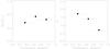 |
Fig. 9 We investigate the possibility that the flattening of the fraction-mass relation (Fig. 8) is caused by the uncertainty on the stellar mass estimates. To do this, we generate X-ray AGN samples characterised by a relation fX = C11Mαwhere C11 and αare free variables. After scattering the stellar mass estimates, we derive χ2 corresponding to each C11and α. This test shows the scatter introduced by the stellar mass uncertainty cannot explain the flattening of the fX − M relation. |
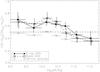 |
Fig. 10 The averaged | V/Vmax | in different stellar mass bins for different galaxy populations. As suggested by the flattening of the fraction-mass relation, the low stellar mass AGN show more evolution than the higher mass ones, as compared to the normal galaxies of the same mass. |
4.5. Infrared properties
In order to study the infrared properties of the optical hosts of X-ray AGN, leading on from Tasse et al. (2008a), we have derived infrared excess parameters at 3.6, 4.5, 5.8, 8.0 μm. This excess is calculated in the observer frame, by computing the logarithmic ratio of the observed flux density to the flux density of the best-fit ZPEG SED template (which does not take into account dust infrared emission), as deduced using fits to the u∗g′r′i′z′ magnitude measurements. In order to compare the infrared excess of the optical hosts of AGN to the infrared excess of the normal galaxy population, we compute the difference between their infrared excesses ΔIRin similar stellar mass and redshift bins (see Tasse et al. 2008a, for details). Figure 11 shows ΔIRfor the Type-2 X-ray selected AGN. As suggested by the distribution of these sources in the infrared [3.6]–[4.5] versus [5.8]–[8.0] colour–colour plot (Fig. 3), X-ray selected AGN show an infrared excess at short wavelength.
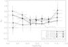 |
Fig. 11 Following Tasse et al. (2008a) we have computed the infrared excess for the normal galaxies and for the host galaxies of X-ray selected AGN. This plot shows the difference in infrared excess between these two populations at fixed redshift and stellar mass. The X-ray selected AGN show a hot infrared excess, at short wavelengths all across the stellar mass range. For comparison we plot the infrared excess computed in a similar way for the radio selected AGN (dashed line, see Tasse et al. 2008a). |
4.6. Environment
In Tasse et al. (2008a) we described an overdensity parameter that is based on the photometric redshift probability functions. It gives the significance of the number density found around a given object at a given comoving scale. Following Tasse et al. (2008a), we have computed the overdensity parameter at 75, 250 and 450 kpc for the sample of X-ray selected AGN, and compare the overdensity of the AGN population with the overdensities of the normal galaxies. In order to compare the environment of distinct populations, for each X-ray selected AGN, we compute the quantity Δρ = ρi − q0.5 [ρN(dz,dM)] , where ρiis the estimated overdensity of the given object and q0.5 [ρN(dz,dM)] is the median overdensity of all galaxies that have comparable stellar mass, and redshift estimates (in practice, we take redshift bin dz = 0.1, and mass bin dM = 0.2). Figure 12 shows the median value of Δρfor the X-ray AGN as a function of stellar mass.
The environment of X-ray AGN is quite different from the environment of normal galaxies. The X-ray AGN are preferentially situated in large scale underdensities (Δρ450 ~ −0.4), while they seem quite insensitive to the small scale environment.
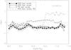 |
Fig. 12 We have computed the overdensity parameter for the normal galaxies and for the X-ray selected AGN. This figure shows the differences between these two populations: the X-ray selected AGN lay in large scale (450 kpc) underdense environments. For comparison we plot the same quantity for the radio selected AGN (dashed line, see Tasse et al. 2008a). |
5. Summary and discussion
In the following we highlight the consistency between the data presented in this paper and the scheme in which the X-ray AGN trace a population of actively accreting AGN. We argue that this class of AGN corresponds to the population of AGN selected by their emission-line luminosity, as well as the radio-loud AGN with radiatively efficient accretion that dominate the radio-loud AGN population at low stellar masses. We finally discuss the connections between the nature of the triggering processes of the AGN activity, and the accretion mode.
In this paper we have proceeded to optically identify a sample of ~1000 point-like X-ray sources in the XMM-LSS field, leading to a fraction of X-ray sources having an optical counterpart of ~80%. In order to reject the Type-1 AGN for which we cannot retrieve reliable photometric redshifts estimates, we have followed in detail the method described in Tasse et al. (2008b). In order to correct for the extinction in the line of sight, we have estimated the hydrogen column density. A significant fraction of our selected Type-2 AGN sample (≳ 40%) shows such absorption in the X-ray, with column densities nH > 1022 cm-2(Fig. 5). These estimates are in good agreement with results from previous surveys (Tajer et al. 2007). Based on these estimates, we have corrected for the extinction, and estimate the intrinsic X-ray luminosities. The X-ray luminosity function of the Type-2 X-ray selected AGN sample in the redshift ranges 0.1 < z < 0.5and 0.5 < z < 1.0(Fig. 7) shows good agreement with previous measurements (Steffen et al. 2003), with a strong comoving number density evolution at L [2−10] > 1043 erg s-1. Following Tasse et al. (2008a) we have computed the stellar mass function, infrared excesses, and overdensity parameters of the host galaxies of Type-2 X-ray sources. The main results are as follows:
-
(i)
At low redshift, the fraction fXof galaxies that are X-ray lumi-nous with LX > 1043 erg s-1has a strongstellar mass dependence with fX ∝ M1.5, which is similar to the slopefound for the emission-line AGN at low stellar masses (Bestet al. 2005). At higher redshift,this relation seems to flatten and to follow the one of the radioselected AGN of low stellar mass (M ≲ 1010.5−11M⊙). The mass-dependent evo-lution is supported by the analysis of the V/Vmaxestimator. By usingan X-ray versus [OIII] luminosity relationship (Heckmanet al. 2005), we found that the co-moving number density of X-ray selected and emission-lineselected AGN differ by ~1 dex at low redshift.That can be explained by our sample missing heavily obscuredsources.
-
(ii)
Compared with normal galaxies of the same mass, X-ray selected AGN show an infrared excess in the IRAC bands (3.6, 4.5, 5.8and 8.0 μm) and over the full mass range (Fig. 11).
-
(iii)
Compared with normal galaxies of the same mass and redshift, X-ray selected AGN tend to be found in underdense large-scale (450 kpc) environments over the full stellar mass range. Their 75 kpc environment is similar to that found around normal galaxies.
As discussed in Sect. 1, many authors have suggested that there are two different modes of accretion: the Quasar mode is characterised by radiative efficiency, while the Radio mode is radiatively inefficient. The analysis of the host galaxies and environment of radio sources hosts presented in Tasse et al. (2008a) suggested the existence of a link between the density of the environment on large scale (~450 kpc) and the nature of the accretion mode. We argued that this link might be caused by the nature of the triggering process being directly connected to the nature of the accretion mode. Specifically, the absence of infrared excess for the radio-loud massive galaxies in our sample (M > 1010.5−11.0 M⊙), is consistent with those AGN accreting in radiatively inefficient mode. Furthermore, the preference of those galaxies to live in higher density environment is consistent with the AGN activity being triggered by the cooling of the hot gas observed in their atmosphere (Mathews & Brighenti 2003; Best et al. 2005). Conversely, the lower stellar mass systems (M < 1010.5−11.0 M⊙) show signs of actively accreting black holes. We have argued that their AGN activity corresponds to a cold gas accretion, triggered by galaxy mergers and interaction in underdense environments. In the following, we argue that the result of this paper confirm that Type-2 X-ray selected AGN correspond to the radiatively efficient Quasar mode.
Result (i) above shows that, as expected, the fraction of galaxies that are X-ray AGN is a strong function of the stellar mass (Fig. 8). This relation shows a flattening in the higher redshift bins, which suggests that the lower mass galaxies (M < 1010.5−11.0 M⊙) play an important role in the evolution of the X-ray luminosity function. The V/Vmaxanalysis seems to support this picture. Using an L [OIII] − LXrelationship (Heckman et al. 2005), the number densities of X-ray selected and emission-line selected AGN show large differences. We have argued in Sect. 4.3 that this effect is indeed expected as many Type-2 emission-line AGN are not seen to produce significant X-ray flux, even in the hard [2–10] keV X-ray bands (Heckman et al. 2005). This is often interpreted as sources that are heavily absorbed and even Compton-thick (Levenson et al. 2002). Although we have corrected for the intrinsic absorption in each individual source, this suggests that there are many obscured X-ray sources, that we simply do not detect. However, at low redshift the slope of the relation between stellar mass and fraction of X-ray selected AGN (fX ∝ M1.5) is in good agreement with the relation between the fraction of galaxies that are classified as AGN using emission-line criteria, while it disagrees with the fraction fRadof radio-loud AGN versus stellar mass relation fRad ∝ M2.5in the high-mass regime. This suggests that although we are missing a significant fraction of the X-ray luminous AGN, we are indeed selecting the same AGN population as that of low-mass emission-line AGN that have been recognised as AGN which have radiatively efficient accretion (“Quasar mode”, Heckman et al. 2004; Best et al. 2005). This picture is supported by the result (ii) on the infrared properties of X-ray selected AGN: these objects have a hot dust component at wavelength as short as 3.6 μm (observer frame), which is often interpreted as being due to an actively accreting black hole where UV light heats the surrounding dust to temperatures of 500−1000 K (Seymour et al. 2007). Result (iii) suggests that these AGN are mainly located in large 450 kpc scale underdensities at levels of ~−0.5. Consistently, luminous L [OIII] > 107 L⊙ emission-line AGN are preferentially found in underdense environment (Kauffmann et al. 2004; Best et al. 2005).
The internal and environmental properties of this X-ray selected AGN population are very similar to the characteristics of the low stellar mass radio selected AGN population. Both of these classes of AGN have a rather flat fraction mass relation (f ∝ M1.5), an infrared excess, they lie in large scale underdense environments, and they show similar evolution. These factors suggest that X-ray, optical, and low-mass radio AGN are similar populations, whose accretion is radiatively efficient. However, environmental differences are found at the smaller scale: contrary to the radio AGN, the X-ray selected AGN seem quite insensitive to their small 75 kpc scale overdensities.
It has often been proposed that luminous AGN activity is triggered by galaxy mergers and interactions, and this process has been suggested to occur more frequently in underdense environments (e.g. Gómez et al. 2003; Best 2004; Gandhi et al. 2006). Galaxy mergers and interactions may provide a natural explanation for the differences found in the 75 kpc scale environment. If the AGN are triggered by a major merger, there might be an observational sequence that AGN follow during their lifetime: while the radio emission is seen to be associated with small scale overdensities, it might be that during the X-ray emitting phase, the two interacting galaxies have already merged into a single system. Alternatively, Taniguchi (1999) suggests that minor mergers that are produced by the interaction between a given galaxy and a low-mass satellite galaxy can play an important role in triggering AGN activity. In such cases our dataset would certainly not allow us to detect a galaxy pair as a small 75 kpc overdensity.
Online material
Appendix A: Table
Properties of the selected Type-2 X-ray sources. (1) X-ray source Name. (2) X-ray source right ascension. (3). X-ray source declination. (4) X-ray source flux in the soft 0.5–2 keV band in erg s-1 cm-2. (5) X-ray source flux in the hard 2–10 keV band in erg s-1 cm-2. (6) Optical counterpart right Ascension (J2000). (7) Optical counterpart declination (J2000). (8) u-band magnitude. Note “NC” means the field has not been observed in that band.(9) g-band magnitude. Note “NC” means the field has not been observed in that band. (10) r-band magnitude. (11) i-band magnitude. (12) z-band magnitude. Note “NC” means the field has not been observed in that band. (13) Estimated probability that the X-ray source is associated with the corresponding optical candidate. (14) 3.6 μm magnitude (AB). Tag “NC” (standing for “Not Covered”) has been used when the location of the object is not overlapping with the SWIRE field. We have used the same notation for the following columns. (15) 4.5 μm magnitude (AB). (16) 5.8 μm magnitude (AB). (17) 8.0 μm magnitude (AB). (18) Photometric redshift as estimated by ZPEG. (19) Stellar mass as estimated by ZPEG in logarithm base-10 scale. (20) Specific SFR as estimated by ZPEG in logarithm base-10 scale. (21) Estimated hydrogen column density in cm-2. (22) Estimated rest-frame intrinsic X-ray luminosity in the 2–10 keV band.
See http://swire.ipac.caltech.edu/swire/ for more information.
If Cis a given criteria, then the observed number of sources satisfying
Cis ![Mathematical equation: \hbox{$n_{\rm obs}(C)=\sum_{\Omega_{i,j}(C)} [P_{id}^i(j)]$}](/articles/aa/full_html/2011/01/aa11129-08/aa11129-08-eq260.png) , where
, where
 is the association probability between the
jthoptical candidate and the ithX-ray source, and
Ωi,j(C)is the set of
{ i,j } optical candidates satisfying C(Tasse et al. 2008b).
is the association probability between the
jthoptical candidate and the ithX-ray source, and
Ωi,j(C)is the set of
{ i,j } optical candidates satisfying C(Tasse et al. 2008b).
The number of optical objects is computed from the sum of association probabilities over the whole selected sample.
To obtain a sample with good photometry with no additional selection, we apply here SC1 and SC2 only.
In Fig. 3, in order to plot the most likely optical counterpart, for each X-ray source, following Tasse et al. (2008b), we consider the optical candidate that has the highest likelihood ratio, provided that it is above the likelihood ratio LRcut = 0.1. Using the probability-weighted number of such rejected sources, we estimate that such sample has reliability and completeness levels of ~90%and ~94%respectively.
Acknowledgments
The optical images were obtained with MegaPrime/MegaCam, a joint project of CFHT and CEA/DAPNIA, at the CFHT which is operated by the National Research Council (NRC) of Canada, the Institut National des Sciences de l’Univers of the Centre National de la Recherche Scientifique (CNRS) of France and the University of Hawaii. This work is based on data products produced at TERAPIX and at the Canadian Astronomy Data Centre as part of the CFHTLS, a collaborative project of NRC and CNRS.
References
- Avni, Y., & Bahcall, J. N. 1980, ApJ, 235, 694 [NASA ADS] [CrossRef] [Google Scholar]
- Benn, C. R. 1983, The Observatory, 103, 150 [NASA ADS] [Google Scholar]
- Best, P. N. 2004, MNRAS, 351, 70 [NASA ADS] [CrossRef] [Google Scholar]
- Best, P. N., Kauffmann, G., Heckman, T. M., et al. 2005, MNRAS, 362, 25 [NASA ADS] [CrossRef] [Google Scholar]
- Best, P. N., Kaiser, C. R., Heckman, T. M., & Kauffmann, G. 2006, MNRAS, 368, L67 [NASA ADS] [Google Scholar]
- Cappi, M., Panessa, F., Bassani, L., et al. 2006, A&A, 446, 459 [NASA ADS] [CrossRef] [EDP Sciences] [Google Scholar]
- Chiappetti, L., Tajer, M., Trinchieri, G., et al. 2005, A&A, 439, 413 [NASA ADS] [CrossRef] [EDP Sciences] [Google Scholar]
- Cowie, L. L., Garmire, G. P., Bautz, M. W., et al. 2002, ApJ, 566, L5 [NASA ADS] [CrossRef] [Google Scholar]
- Croton, D. J., Springel, V., White, S. D. M., et al. 2006, MNRAS, 365, 11 [NASA ADS] [CrossRef] [Google Scholar]
- de Ruiter, H. R., Arp, H. C., & Willis, A. G. 1977, A&AS, 28, 211 [NASA ADS] [Google Scholar]
- Dickey, J. M., & Lockman, F. J. 1990, ARA&A, 28, 215 [NASA ADS] [CrossRef] [MathSciNet] [Google Scholar]
- Gandhi, P., Garcet, O., Disseau, L., et al. 2006, The XMM large scale structure survey: properties and two-point angular correlations of point-like sources [Google Scholar]
- Gómez, P. L., Nichol, R. C., Miller, C. J., et al. 2003, ApJ, 584, 210 [NASA ADS] [CrossRef] [Google Scholar]
- Hardcastle, M. J., Evans, D. A., & Croston, J. H. 2006, MNRAS, 370, 1893 [NASA ADS] [CrossRef] [Google Scholar]
- Hardcastle, M. J., Evans, D. A., & Croston, J. H. 2007, MNRAS, 376, 1849 [NASA ADS] [CrossRef] [Google Scholar]
- Heckman, T. M., & Kauffmann, G. 2006, New Astron. Rev., 50, 677 [NASA ADS] [CrossRef] [Google Scholar]
- Heckman, T. M., Kauffmann, G., Brinchmann, J., et al. 2004, ApJ, 613, 109 [NASA ADS] [CrossRef] [Google Scholar]
- Heckman, T. M., Ptak, A., Hornschemeier, A., & Kauffmann, G. 2005, ApJ, 634, 161 [NASA ADS] [CrossRef] [Google Scholar]
- Hine, R. G., & Longair, M. S. 1979, MNRAS, 188, 111 [NASA ADS] [Google Scholar]
- Jackson, N., & Rawlings, S. 1997, MNRAS, 286, 241 [NASA ADS] [CrossRef] [Google Scholar]
- Kauffmann, G., White, S. D. M., Heckman, T. M., et al. 2004, MNRAS, 353, 713 [NASA ADS] [CrossRef] [Google Scholar]
- Le Borgne, D., & Rocca-Volmerange, B. 2002, A&A, 386, 446 [NASA ADS] [CrossRef] [EDP Sciences] [Google Scholar]
- Levenson, N. A., Krolik, J. H., Życki, P. T., et al. 2002, ApJ, 573, L81 [NASA ADS] [CrossRef] [Google Scholar]
- Liu, B. F., Mineshige, S., Meyer, F., Meyer-Hofmeister, E., & Kawaguchi, T. 2002, ApJ, 575, 117 [NASA ADS] [CrossRef] [Google Scholar]
- Lonsdale, C. J., Smith, H. E., Rowan-Robinson, M., et al. 2003, PASP, 115, 897 [NASA ADS] [CrossRef] [Google Scholar]
- Mathews, W. G., & Brighenti, F. 2003, ARA&A, 41, 191 [NASA ADS] [CrossRef] [Google Scholar]
- Ogle, P., Whysong, D., & Antonucci, R. 2006, ApJ, 647, 161 [NASA ADS] [CrossRef] [Google Scholar]
- Pacaud, F., Pierre, M., Refregier, A., et al. 2006, MNRAS, 372, 578 [NASA ADS] [CrossRef] [Google Scholar]
- Pierre, M., Valtchanov, I., Altieri, B., et al. 2004, J. Cosmol. Astropart. Phys., 9, 11 [Google Scholar]
- Polletta, M. D. C., Wilkes, B. J., Siana, B., et al. 2006, ApJ, 642, 673 [NASA ADS] [CrossRef] [Google Scholar]
- Prestage, R. M., & Peacock, J. A. 1983, MNRAS, 204, 355 [NASA ADS] [Google Scholar]
- Reynolds, C. S. 1997, MNRAS, 286, 513 [NASA ADS] [CrossRef] [Google Scholar]
- Richter, G. A. 1975, Astron. Nachr., 296, 65 [NASA ADS] [CrossRef] [Google Scholar]
- Risaliti, G., Maiolino, R., & Salvati, M. 1999, ApJ, 522, 157 [NASA ADS] [CrossRef] [Google Scholar]
- Sazonov, S. Y., & Revnivtsev, M. G. 2004, A&A, 423, 469 [NASA ADS] [CrossRef] [EDP Sciences] [Google Scholar]
- Schmidt, M. 1968, ApJ, 151, 393 [NASA ADS] [CrossRef] [Google Scholar]
- Seymour, N., Stern, D., De Breuck, C., et al. 2007, ApJS, 171, 353 [NASA ADS] [CrossRef] [Google Scholar]
- Springel, V., Di Matteo, T., & Hernquist, L. 2005, ApJ, 620, L79 [NASA ADS] [CrossRef] [Google Scholar]
- Stalin, C. S., Petitjean, P., Srianand, R., et al. 2010, MNRAS, 401, 294 [NASA ADS] [CrossRef] [Google Scholar]
- Steffen, A. T., Barger, A. J., Cowie, L. L., Mushotzky, R. F., & Yang, Y. 2003, ApJ, 596, L23 [NASA ADS] [CrossRef] [Google Scholar]
- Stern, D., Eisenhardt, P., Gorjian, V., et al. 2005, ApJ, 631, 163 [NASA ADS] [CrossRef] [Google Scholar]
- Surace, J. A., Shupe, D. L., Fang, F., et al. 2004, VizieR Online Data Catalog, 2255, [Google Scholar]
- Sutherland, W., & Saunders, W. 1992, MNRAS, 259, 413 [NASA ADS] [CrossRef] [Google Scholar]
- Tajer, M., Polletta, M., Chiappetti, L., et al. 2007, A&A, 467, 73 [NASA ADS] [CrossRef] [EDP Sciences] [Google Scholar]
- Taniguchi, Y. 1999, ApJ, 524, 65 [NASA ADS] [CrossRef] [Google Scholar]
- Tasse, C., Cohen, A. S., Röttgering, H. J. A., et al. 2006, A&A, 456, 791 [NASA ADS] [CrossRef] [EDP Sciences] [Google Scholar]
- Tasse, C., Röttgering, H. J. A., Best, P. N., et al. 2007, A&A, 471, 1105 [NASA ADS] [CrossRef] [EDP Sciences] [Google Scholar]
- Tasse, C., Best, P. N., Röttgering, H., & Le Borgne, D. 2008a, A&A, 490, 893 [NASA ADS] [CrossRef] [EDP Sciences] [Google Scholar]
- Tasse, C., Le Borgne, D., Röttgering, H., et al. 2008b, A&A, 490, 879 [NASA ADS] [CrossRef] [EDP Sciences] [Google Scholar]
- Wolstencroft, R. D., Savage, A., Clowes, R. G., et al. 1986, MNRAS, 223, 279 [NASA ADS] [Google Scholar]
All Tables
Properties of the selected Type-2 X-ray sources. (1) X-ray source Name. (2) X-ray source right ascension. (3). X-ray source declination. (4) X-ray source flux in the soft 0.5–2 keV band in erg s-1 cm-2. (5) X-ray source flux in the hard 2–10 keV band in erg s-1 cm-2. (6) Optical counterpart right Ascension (J2000). (7) Optical counterpart declination (J2000). (8) u-band magnitude. Note “NC” means the field has not been observed in that band.(9) g-band magnitude. Note “NC” means the field has not been observed in that band. (10) r-band magnitude. (11) i-band magnitude. (12) z-band magnitude. Note “NC” means the field has not been observed in that band. (13) Estimated probability that the X-ray source is associated with the corresponding optical candidate. (14) 3.6 μm magnitude (AB). Tag “NC” (standing for “Not Covered”) has been used when the location of the object is not overlapping with the SWIRE field. We have used the same notation for the following columns. (15) 4.5 μm magnitude (AB). (16) 5.8 μm magnitude (AB). (17) 8.0 μm magnitude (AB). (18) Photometric redshift as estimated by ZPEG. (19) Stellar mass as estimated by ZPEG in logarithm base-10 scale. (20) Specific SFR as estimated by ZPEG in logarithm base-10 scale. (21) Estimated hydrogen column density in cm-2. (22) Estimated rest-frame intrinsic X-ray luminosity in the 2–10 keV band.
All Figures
|
Fig. 1 The location of the CFHTLS, SWIRE, XMM-LSS fields. The black dots show the X-ray sources selected for optical and infrared identification. |
| In the text | |
|
Fig. 2 In order to identify the optical counterparts of X-ray AGN, we take into account the magnitude distribution of X-ray sources hosts, which is different from that of the confusing background sources. The estimated fraction (y-axis) of X-ray AGN having an optical counterpart with i-band below magnitude m(x-axis), has been determined using a Monte-Carlo simulation (see Tasse et al. 2008b, for the details). Around 76%of X-ray sources have an optical counterpart at the limiting magnitude of our survey (the vertical dotted line shows the 80% completeness level of the optical survey). |
| In the text | |
|
Fig. 3 Top panel: the g′ − r′versus r′ − i′ colour–colour diagram for all the optical counterparts of X-ray sources (black dots, applying selection criteria SC1 and SC2 only6). Open circles indicate the optical counterparts of X-ray sources that have been classified as Type-1 AGN by the spectral fit criteria using the IRAC bands (SC6). The dashed area indicates the region corresponding to the optical g′ − r′versus r′ − i′ selection criteria used to reject the contaminating Type-1 AGN (SC5, grey diamonds). Radio source host galaxies (indicated by crosses) and X-ray optical counterparts clearly occupy different regions of this plot, with the radio-loud AGN more typically hosted by galaxies that do not show strong signs of AGN activity in the optical. We also plot the colour-colour tracks for a Type-1 QSO, an elliptical, and a starburst galaxy. The square, star, diamond and triangle symbols stand for redshifts 0, 0.5, 1.5, and 2 respectively. Bottom panel: the [3.6]–[4.5] versus [5.8]–[8.0] infrared colour–colour diagram. Stern et al. (2005) find ~90%of the broad-line AGN lying in the area delimited by the dotted line. Symbols are as in the top panel. The sources marked as open circles and diamonds have been rejected from our sample. |
| In the text | |
|
Fig. 4 Hardness ratio distribution for the sources that have been selected (Type-2) and rejected (Type-1). As is expected, the sources showing signs of absorption in the optical and infrared domains have higher hardness ratios. |
| In the text | |
|
Fig. 5 Based on the observed flux ratio F [0.5−2] /F [2−10] , assuming an underlying Fν ∝ ν-0.8X-ray spectra, we have estimated the hydrogen column density for the sample of Type-2 AGN selected in Sect. 3.2. The shaded region shows the fraction of sources in our sample that have hydrogen column density lower than 1020 cm-2. As expected, most of the AGN we have selected show signs of absorption in their X-ray spectra. |
| In the text | |
|
Fig. 6 The cumulative distribution of the difference between our estimate of the photometric redshift and the spectroscopic redshift as measured by Stalin et al. (2010). The dashed line shows a normal distribution with σ(Δz) = 0.1. |
| In the text | |
|
Fig. 7 We have estimated the X-ray luminosity function in the 0.1 < z < 0.5and 0.5 < z < 1.0redshift bins. Our estimates are in good agreement with the results presented in Steffen et al. (2003). |
| In the text | |
|
Fig. 8 The fraction of galaxies that are X-ray AGN with L [2−10] > 1043 erg s-1, as a function of the stellar mass, in the 0.1 < z < 1.2, 0.1 < z < 0.6, 0.4 < z < 0.9and 0.7 < z < 1.2redshift ranges. At low redshift the slope of the relationship shows good agreement with the fraction of galaxies that are classified as AGN based on emission-line criteria (Best et al. 2005), while it seems to evolve in the same way as the radio-loud fraction of galaxies at low stellar masses. |
| In the text | |
|
Fig. 9 We investigate the possibility that the flattening of the fraction-mass relation (Fig. 8) is caused by the uncertainty on the stellar mass estimates. To do this, we generate X-ray AGN samples characterised by a relation fX = C11Mαwhere C11 and αare free variables. After scattering the stellar mass estimates, we derive χ2 corresponding to each C11and α. This test shows the scatter introduced by the stellar mass uncertainty cannot explain the flattening of the fX − M relation. |
| In the text | |
|
Fig. 10 The averaged | V/Vmax | in different stellar mass bins for different galaxy populations. As suggested by the flattening of the fraction-mass relation, the low stellar mass AGN show more evolution than the higher mass ones, as compared to the normal galaxies of the same mass. |
| In the text | |
|
Fig. 11 Following Tasse et al. (2008a) we have computed the infrared excess for the normal galaxies and for the host galaxies of X-ray selected AGN. This plot shows the difference in infrared excess between these two populations at fixed redshift and stellar mass. The X-ray selected AGN show a hot infrared excess, at short wavelengths all across the stellar mass range. For comparison we plot the infrared excess computed in a similar way for the radio selected AGN (dashed line, see Tasse et al. 2008a). |
| In the text | |
|
Fig. 12 We have computed the overdensity parameter for the normal galaxies and for the X-ray selected AGN. This figure shows the differences between these two populations: the X-ray selected AGN lay in large scale (450 kpc) underdense environments. For comparison we plot the same quantity for the radio selected AGN (dashed line, see Tasse et al. 2008a). |
| In the text | |
Current usage metrics show cumulative count of Article Views (full-text article views including HTML views, PDF and ePub downloads, according to the available data) and Abstracts Views on Vision4Press platform.
Data correspond to usage on the plateform after 2015. The current usage metrics is available 48-96 hours after online publication and is updated daily on week days.
Initial download of the metrics may take a while.