| Issue |
A&A
Volume 524, December 2010
|
|
|---|---|---|
| Article Number | A22 | |
| Number of page(s) | 13 | |
| Section | Planets and planetary systems | |
| DOI | https://doi.org/10.1051/0004-6361/201015177 | |
| Published online | 22 November 2010 | |
Stochastic orbital migration of small bodies in Saturn’s rings⋆
University of Cambridge, Department of Applied Mathematics and
Theoretical Physics, Centre for Mathematical Sciences, Wilberforce Road, Cambridge
CB3 0WA,
UK
e-mail: This email address is being protected from spambots. You need JavaScript enabled to view it.
Received:
8
June
2010
Accepted:
11
August
2010
Abstract
Many small moonlets that create propeller structures have been found in Saturn’s rings by the Cassini spacecraft. We study the dynamical evolution of such 20−50 m sized bodies, which are embedded in Saturn’s rings. We estimate the importance of various interaction processes with the ring particles on the moonlet’s eccentricity and semi-major axis analytically. For low ring surface densities, the main effects on the evolution of the eccentricity and the semi-major axis are found to be caused by collisions and the gravitational interaction with particles in the vicinity of the moonlet. For high surface densities, the gravitational interaction with self-gravity wakes becomes important.
We also perform realistic three-dimensional, collisional N-body simulations with up to a quarter of a million particles. A new set of pseudo shear periodic boundary conditions is used, which reduces the computational costs by an order of magnitude compared to previous studies. Our analytic estimates are confirmed to within a factor of two.
On short timescales the evolution is always dominated by stochastic effects caused by collisions and gravitational interaction with self-gravitating ring particles. These result in a random walk of the moonlet’s semi-major axis. The eccentricity of the moonlet quickly reaches an equilibrium value owing to collisional damping. The average change in semi-major axis of the moonlet after 100 orbital periods is 10-100 m. This translates to an offset in the azimuthal direction of several hundred kilometres. We expect that such a shift is easily observable.
Key words: celestial mechanics / planets and satellites: rings / planets and satellites: dynamical evolution and stability / planet-disk interactions
Two movies are only available in electronic form at http://www.aanda.org
© ESO, 2010
1. Introduction
Small bodies called moonlets, which are embedded in Saturn’s rings, can create propeller-shaped structures by disturbing the rings. These have been predicted both analytically and numerically (Spahn & Sremčević 2000; Sremčević et al. 2002; Seiß et al. 2005). Only recently have they been observed by the Cassini spacecraft in both the A and B rings (Tiscareno et al. 2006, 2008).
These 20−100 m sized bodies can migrate within the rings, similar to protoplanets that migrate in a protostellar disc. Depending on the disc properties and the moonlet size, this can happen in either a smooth or in a stochastic (random-walk) fashion. We refer to those migration regimes as types I and IV, respectively, in analogy to the terminology in disc-planet interactions. Crida et al. (2010) show that, in the case of a laminar disc, there is a type I regime that might be important on very long timescales. This migration is qualitatively different to the migration in a pressure supported gas disc. However, the migration of moonlets in the A ring is generally dominated by type IV migration, at least on short timescales.
In this paper, we study the type IV migration regime in detail. The full mutual interaction of the ring particles with the moonlet and its consequent induced motion are considered both analytically and numerically.
We first review the basic equations governing the moonlet and the ring particles in a shearing box approximation in Sect. 2. Then, in Sect. 3, we estimate the eccentricity damping timescale due to ring particles colliding with the moonlet and ring particles on horseshoe orbits, as well as the effect of particles on circulating orbits. In Sect. 4 we estimate the excitation of the moonlet eccentricity caused by stochastic particle collisions and gravitational interactions with ring particles. This enables us to derive an analytic estimate of the equilibrium eccentricity. In Sect. 5 we discuss and evaluate processes, such as collisions and gravitational interactions with ring particles and self-gravitating clumps, which lead to a random walk in the semi-major axis of the moonlet.
We describe our numerical code and the initial conditions used in Sect. 6. We perform realistic three dimensional N-body simulations of the ring system and the moonlet, taking into account a moonlet with finite size, a size distribution of ring particles, self-gravity, and collisions. The results are presented in Sect. 7. All analytic estimates are confirmed both in terms of qualitative trends and quantitatively to within a factor of about two in all the simulations that we performed. We also discuss the long-term evolution of the longitude of the moonlet and its observability, before summarising our results in Sect. 8.
2. Basic equations governing the moonlet and ring particles
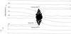 |
Fig. 1 Trajectories of ring particles in a frame centred on the moonlet. Particles accumulate near the moonlet and fill its Roche lobe. Particles on trajectories labelled (a) are on circulating orbits. Particles on trajectories labelled (b) collide with other particles in the moonlet’s vicinity. Particles on trajectories labelled (c) collide with the moonlet directly. Particles on trajectories labelled (d) are on horseshoe orbits. Particles on trajectories labelled (e) leave the vicinity of the moonlet. |
We adopt a local right-handed Cartesian coordinate system with its origin in a circular Keplerian orbit with semi-major axis a and rotating uniformly with angular velocity Ω. This orbit coincides with that of the moonlet when it is assumed to be unperturbed by ring particles. The x axis coincides with the line joining the central object of mass Mp and the origin. The unit vector in the x direction ex, points away from the central object. The unit vector in the y direction ey, points in the direction of rotation and the unit vector in the z direction, ez, points in the vertical direction being normal to the disc mid-plane.
In general, we consider a ring particle of mass m1 interacting with the moonlet that has a much higher mass m2. A sketch of three possible types of particle trajectory in the vicinity of the moonlet is shown in Fig. 1. These correspond to three distinct regimes, a) denoting circulating orbits, b) and c) denoting orbits that result in a collision with particles in the vicinity of the moonlet and directly with the moonlet, respectively, and d) denoting horseshoe orbits. All these types of trajectories occur for particles that are initially in circular orbits, both interior and exterior to the moonlet, when at large distances from it.
Approximating the gravitational force due to the central object by its first-order Taylor
expansion about the origin leads to Hill’s equation, governing the motion of a particle of
mass m1 of the form
 (1)where
r = (x,y,z) is position of a particle
with mass m1, and Ψ is the gravitational potential acting on the
particle due to other objects such as the moonlet.
(1)where
r = (x,y,z) is position of a particle
with mass m1, and Ψ is the gravitational potential acting on the
particle due to other objects such as the moonlet.
The square amplitude of the epicyclic motion ℰ2 can be defined through
 (2)Note
that neither the eccentricity e nor the semi-major axis a
are formally defined in the local coordinate system. However, in the absence of any
interaction with other masses (Ψ = 0), ℰ is conserved, and up to first
order in the eccentricity we may make the identification
ℰ = ea. We recall the classical definition of the
eccentricity e in a coordinate system centred on the central object
(2)Note
that neither the eccentricity e nor the semi-major axis a
are formally defined in the local coordinate system. However, in the absence of any
interaction with other masses (Ψ = 0), ℰ is conserved, and up to first
order in the eccentricity we may make the identification
ℰ = ea. We recall the classical definition of the
eccentricity e in a coordinate system centred on the central object
 (3)Here,
s is the position vector
(a,0,0), and w is the
velocity vector of the particle relative to the mean shear associated with circular
Keplerian motion as viewed in the local coordinate system plus the circular Keplerian
velocity corresponding to the orbital frequency Ω of the origin. Thus,
(3)Here,
s is the position vector
(a,0,0), and w is the
velocity vector of the particle relative to the mean shear associated with circular
Keplerian motion as viewed in the local coordinate system plus the circular Keplerian
velocity corresponding to the orbital frequency Ω of the origin. Thus,
 (4)All
eccentricities considered here are very small ( ~ 10-8−10-7) so that
the difference between the quantities defined through use of Eqs. (2) and (3) is negligible, allowing us to adopt ℰ as a measure of the eccentricity
throughout this paper.
(4)All
eccentricities considered here are very small ( ~ 10-8−10-7) so that
the difference between the quantities defined through use of Eqs. (2) and (3) is negligible, allowing us to adopt ℰ as a measure of the eccentricity
throughout this paper.
Let us define another quantity,  , that is also conserved for
non-interacting particle motion, Ψ = 0, which is the x
coordinate of the centre of the epicyclic motion and is given by
, that is also conserved for
non-interacting particle motion, Ψ = 0, which is the x
coordinate of the centre of the epicyclic motion and is given by
 (5)We
identify a change in
(5)We
identify a change in  as a change in the semi-major axis
a of the particle, again, under the assumption that the eccentricity is
small.
as a change in the semi-major axis
a of the particle, again, under the assumption that the eccentricity is
small.
2.1. Two interacting particles
We now consider the motion of two gravitationally interacting particles with position
vectors
r1 = (x1,y1,z1)
and
r2 = (x2,y2,z2).
Their corresponding masses are m1 and
m2. The governing equations of motion are
 where
the interaction gravitational potential is
Ψ12 = −Gm1m2/|r1 − r2|.
The position vector of the centre of mass of the two particles is given by
where
the interaction gravitational potential is
Ψ12 = −Gm1m2/|r1 − r2|.
The position vector of the centre of mass of the two particles is given by
 (8)The
vector
(8)The
vector  also obeys Eq. (1) with Ψ = 0, which applies to an isolated
particle, because the interaction potential does not affect the motion of the centre of
mass. We also find it useful to define the vector
also obeys Eq. (1) with Ψ = 0, which applies to an isolated
particle, because the interaction potential does not affect the motion of the centre of
mass. We also find it useful to define the vector
 (9)Then,
consistently with our earlier definition of ℰ, we have
ℰi = |ℰi| . The
amplitude of the epicyclic motion of the centre of mass
(9)Then,
consistently with our earlier definition of ℰ, we have
ℰi = |ℰi| . The
amplitude of the epicyclic motion of the centre of mass  is
given by
is
given by  (10)Here
φ12 is the angle between
E1 and
E2. It is important to note
that is conserved even if the two particles approach
each other and become bound. This is true as long as frictional forces are internal to the
two particle system and do not affect the centre of mass motion.
(10)Here
φ12 is the angle between
E1 and
E2. It is important to note
that is conserved even if the two particles approach
each other and become bound. This is true as long as frictional forces are internal to the
two particle system and do not affect the centre of mass motion.
3. Effects leading to damping of the eccentricity of the moonlet
We begin by estimating the moonlet eccentricity damping rate associated with ring particles that either collide directly with the moonlet, particles in its vicinity, or only interact gravitationally with the moonlet.
3.1. The contribution due to particles impacting the moonlet
Particles hitting the moonlet in an eccentric orbit exchange momentum with it. Let us
assume that a ring particle, identified with m1 has zero
epicyclic amplitude, so that ℰ1 = 0 far away from the moonlet. The moonlet is
identified with m2 and has an initial epicyclic amplitude
ℰ2. The epicyclic amplitude of the centre of mass is therefore  (11)where
we have assumed that m1 ≪ m2.
(11)where
we have assumed that m1 ≪ m2.
The moonlet is assumed to be in a steady state where there is no net accretion of ring particles. Therefore, for every particle that either collides directly with the moonlet or nearby particles bound to it (and so itself becomes temporarily bound to it), one particle must also escape from the moonlet. This happens primarily through slow leakage from locations close to the L1 and L2 points such that most particles escape from the moonlet with almost zero velocity (as viewed from the centre of mass frame) and so do not change its orbital eccentricity. However, after an impacting particle becomes bound to the moonlet, conservation of the epicyclic amplitude associated with the centre of mass motion, together with Eq. (11), imply that each impacting particle will reduce the eccentricity by a factor 1 − m1/m2.
It is now an easy task to estimate the eccentricity damping timescale by determining the number of particle collisions per time unit with the moonlet or particles bound to it. To do that, a smooth window function Wb + c(b) is used, being unity for impact parameters b that always result in an impact with the moonlet or particles nearby that are bound to it, and being zero for impact parameters that never result in an impact.
The number of particles impacting the moonlet per time unit,
dN/dt, is obtained by integrating
over the impact parameter with the result that  (12)where
Σ is the surface mass density. Allowing b to be negative enables impacts
from both sides of the moonlet to be taken into account.
(12)where
Σ is the surface mass density. Allowing b to be negative enables impacts
from both sides of the moonlet to be taken into account.
Therefore, after using Eq. (11), we find
that the rate of change of the moonlet’s eccentricity e2, or
equivalently of its amplitude of epicyclic motion ℰ2, is given by  (13)where
τe,collisions defines the circularisation
time arising from collisions with the moonlet. The natural unit for b is
the Hill radius of the moonlet,
rH = (m2/(3Mp))1/3a,
so that the dimensional scaling for
τe,collisions is given by
(13)where
τe,collisions defines the circularisation
time arising from collisions with the moonlet. The natural unit for b is
the Hill radius of the moonlet,
rH = (m2/(3Mp))1/3a,
so that the dimensional scaling for
τe,collisions is given by  (14)which
we find to also apply to all the processes for modifying the moonlet’s eccentricity
discussed below. If we assume that
Wb + c(|b|) can be approximated by a
box function, being unity in the interval
[1.5rH,2.5rH]
and zero elsewhere, we get
(14)which
we find to also apply to all the processes for modifying the moonlet’s eccentricity
discussed below. If we assume that
Wb + c(|b|) can be approximated by a
box function, being unity in the interval
[1.5rH,2.5rH]
and zero elsewhere, we get  (15)
(15)
3.2. Eccentricity damping due to the interaction of the moonlet with particles on horseshoe orbits
The eccentricity of the moonlet manifests itself in a small oscillation of the moonlet about the origin. Primarily ring particles on horseshoe orbits will respond to that oscillation and damp it. This is because only those particles on horseshoe orbits spend enough time in the vicinity of the moonlet, i.e. many epicyclic periods.
In Appendix A, we calculate the amplitude of
epicyclic motion ℰ1f (or equivalently the eccentricity
e1f) that is induced in a single ring
particle in a horseshoe orbit undergoing a close approach to a moonlet that is assumed to
be in an eccentric orbit. In order to calculate the circularisation time, we have to
consider all relevant impact parameters. We begin by noting that each particle encounter
with the moonlet is conservative and is such that for each particle, the Jacobi constant,
applicable when the moonlet is in a circular orbit, is increased by an amount
 by
the action of the perturbing force, associated with the eccentricity of the moonlet, as
the particle passes by. Because the Jacobi constant, or energy in the rotating frame, for
the moonlet and the particle together is conserved, the square of the epicyclic amplitude
associated with the moonlet alone changes by
by
the action of the perturbing force, associated with the eccentricity of the moonlet, as
the particle passes by. Because the Jacobi constant, or energy in the rotating frame, for
the moonlet and the particle together is conserved, the square of the epicyclic amplitude
associated with the moonlet alone changes by  Accordingly the change in the amplitude of
epicyclic motion of the moonlet ℰ2, consequent on inducing the amplitude of
epicyclic motion ℰ1f in the horseshoe particle, is given by
Accordingly the change in the amplitude of
epicyclic motion of the moonlet ℰ2, consequent on inducing the amplitude of
epicyclic motion ℰ1f in the horseshoe particle, is given by
 (16)Note
that this is different compared to Eq. (11). Here, we are dealing with a second-order effect. First, the eccentric moonlet
excites eccentricity in a ring particle. Second, because the total epicyclic motion is
conserved, the epicyclic motion of the moonlet is reduced.
(16)Note
that this is different compared to Eq. (11). Here, we are dealing with a second-order effect. First, the eccentric moonlet
excites eccentricity in a ring particle. Second, because the total epicyclic motion is
conserved, the epicyclic motion of the moonlet is reduced.
Integrating over the impact parameters associated with ring particles and taking
particles streaming by the moonlet from both directions into account by allowing negative
impact parameters gives  (17)where
τe,horseshoe is the circularisation time
and, as above, we have inserted a window function, which is unity on impact parameters
that lead to horseshoe orbits, otherwise being zero. Using ℰ1f
given by Eq. (A.20), we obtain
(17)where
τe,horseshoe is the circularisation time
and, as above, we have inserted a window function, which is unity on impact parameters
that lead to horseshoe orbits, otherwise being zero. Using ℰ1f
given by Eq. (A.20), we obtain
 (18)For
a sharp cutoff of Wd(b) at
bm = 1.5rH we find the value of
the integral in the above to be 2.84. Thus, in this case we get
(18)For
a sharp cutoff of Wd(b) at
bm = 1.5rH we find the value of
the integral in the above to be 2.84. Thus, in this case we get  (19)However,
note that this value is sensitive to the value of bm adopted.
For
bm = 1.25rH,τe,horseshoe
is a factor of 4.25 larger.
(19)However,
note that this value is sensitive to the value of bm adopted.
For
bm = 1.25rH,τe,horseshoe
is a factor of 4.25 larger.
3.3. The effects of circulating particles
The effect of the response of circulating particles to the gravitational perturbation of the moonlet on the moonlet’s eccentricity can be estimated from the work of Goldreich & Tremaine (1980, 1982). These authors consider a ring separated from a satellite such that co-orbital effects are not considered. Thus, their expressions may be applied to estimate effects of circulating particles. However, we exclude their corotation torques because they are determined by the ring edges and are absent in a local model with uniform azimuthally-averaged surface density. Equivalently, one may simply assume that the corotation torques are saturated. When this is done only Lindblad torques act on the moonlet. These tend to excite the moonlet’s eccentricity rather than damp it.
We replace the ring mass in Eq. (70) of Goldreich
& Tremaine (1982) by the integral over the impact parameter and switch to
our notation to obtain 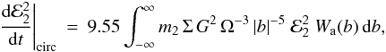 (20)where
Wa(b) is the appropriate window function
for circulating particles. Assuming a sharp cutoff of
Wa( | b | ) at
bm, we can evaluate the integral in Eq. (20) to get
(20)where
Wa(b) is the appropriate window function
for circulating particles. Assuming a sharp cutoff of
Wa( | b | ) at
bm, we can evaluate the integral in Eq. (20) to get 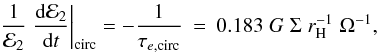 (21)where
we have adopted bm = 2.5rH,
consistent with the simulation results presented below. We see that, although
τe,circ < 0
corresponds to growth rather than damping of the eccentricity, it scales in the same
manner as the circularisation times in Sects. 3.1
and 3.2 scale (see Eq. (14)).
(21)where
we have adopted bm = 2.5rH,
consistent with the simulation results presented below. We see that, although
τe,circ < 0
corresponds to growth rather than damping of the eccentricity, it scales in the same
manner as the circularisation times in Sects. 3.1
and 3.2 scale (see Eq. (14)).
This timescale and the timescale associated with particles on horseshoe orbits, τe,horseshoe, are significantly larger than the timescale associated with collisions, given in Eq. (15). We can therefore ignore those effects for most of the discussion in this paper.
4. Processes leading to the excitation of the eccentricity of the moonlet
In Sect. 3 we assumed that the moonlet had a small eccentricity but neglected the initial eccentricity of the impacting ring particles. When this is included, collisions and gravitational interactions of ring particles with the moonlet may also excite its eccentricity.
4.1. Collisional eccentricity excitation
To see this, assume that the moonlet initially has zero eccentricity, or equivalently no
epicyclic motion, but the ring particles do. As above we consider the conservation of the
epicyclic motion of the centre of mass in order to connect the amplitude of the final
epicyclic motion of the combined moonlet and ring particle to the initial amplitude of the
ring particle’s epicyclic motion. This gives the epicyclic amplitude of the centre of mass
after one impact as 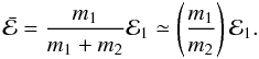 (22)Assuming
that successive collisions are uncorrelated and occur stochastically with the mean time
between consecutive encounters being τce, the evolution of
(22)Assuming
that successive collisions are uncorrelated and occur stochastically with the mean time
between consecutive encounters being τce, the evolution of
 is governed by the equation
 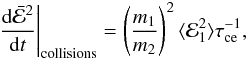 (23)where
 can
be expressed in terms of the surface density and an impact window function
Wb + c(b) (see Eq. (12)). The quantity
can
be expressed in terms of the surface density and an impact window function
Wb + c(b) (see Eq. (12)). The quantity  is the mean square value of ℰ1 for
the ring particles. Using Eq. (2), this may
be written in terms of the mean squares of the components of the velocity dispersion
relative to the background shear, in the form
is the mean square value of ℰ1 for
the ring particles. Using Eq. (2), this may
be written in terms of the mean squares of the components of the velocity dispersion
relative to the background shear, in the form
 (24)We
find ⟨ e1 ⟩ ~ 10-6 in numerical simulations for
almost all ring parameters. This value is mainly determined by the coefficient of
restitution (see e.g. Fig. 4 in Morishima & Salo
2006).
(24)We
find ⟨ e1 ⟩ ~ 10-6 in numerical simulations for
almost all ring parameters. This value is mainly determined by the coefficient of
restitution (see e.g. Fig. 4 in Morishima & Salo
2006).
4.2. Stochastic excitation by circulating particles
Ring particles that are on circulating orbits, as given by path (a) in Fig. 1, exchange energy and angular momentum with the moonlet
and therefore change its eccentricity. Goldreich &
Tremaine (1982) calculated the change in the eccentricity of a ring particle due
to a satellite. We are interested in the change of the eccentricity of the moonlet induced
by a ring of particles and therefore swap the satellite mass with the mass of a ring
particle. Thus, rewriting their results (Eq. (64) in Goldreich & Tremaine 1982) in our local notation without reference to
the semi-major axis, we have  (25)Supposing
that the moonlet has very small eccentricity, it will receive stochastic impulses that
cause its eccentricity to undergo a random walk that will result in
(25)Supposing
that the moonlet has very small eccentricity, it will receive stochastic impulses that
cause its eccentricity to undergo a random walk that will result in
 increasing linearly with
time, so that we may write
increasing linearly with
time, so that we may write  (26)where
d(1/tb) is the mean encounter rate with
particles that have an impact parameter in the interval
(b,b + db) and
Wa(b) is the window function describing the
band of particles in circulating orbits. Setting
d(1/tb) = 3ΣΩ | b | db/(2m1),
we obtain
(26)where
d(1/tb) is the mean encounter rate with
particles that have an impact parameter in the interval
(b,b + db) and
Wa(b) is the window function describing the
band of particles in circulating orbits. Setting
d(1/tb) = 3ΣΩ | b | db/(2m1),
we obtain  (27)For
high surface densities, an additional effect can excite the eccentricity when self-gravity
wakes occur. The Toomre parameter Q is defined as
(27)For
high surface densities, an additional effect can excite the eccentricity when self-gravity
wakes occur. The Toomre parameter Q is defined as
 (28)where
 is the velocity dispersion of the ring
particles1. When the surface density is high enough
for Q to approach unity, transient clumps will form in the rings. The
typical length scale of these structures is given by the critical Toomre wave length
λT = 2π2GΣΩ-2
(Daisaka et al. 2001), which can be used to
estimate a typical mass of the clump:
is the velocity dispersion of the ring
particles1. When the surface density is high enough
for Q to approach unity, transient clumps will form in the rings. The
typical length scale of these structures is given by the critical Toomre wave length
λT = 2π2GΣΩ-2
(Daisaka et al. 2001), which can be used to
estimate a typical mass of the clump:
 (29)Whenever
strong clumping occurs, mT should be used in the above
calculation instead of the mass of a single particle m1:
(29)Whenever
strong clumping occurs, mT should be used in the above
calculation instead of the mass of a single particle m1:
 (30)where
 is the appropriate window function. For typical
parameters used in Sect. 7, this transition occurs
at Σ ~ 200 kg/m2.
is the appropriate window function. For typical
parameters used in Sect. 7, this transition occurs
at Σ ~ 200 kg/m2.
4.3. Equilibrium eccentricity
Putting together the results from this and the previous section, we can estimate an
equilibrium eccentricity of the moonlet. Let us assume that the eccentricity
e2, or the amplitude of the epicyclic motion ℰ2,
evolves under the influence of excitation and damping forces as  (31)Both
the excitation terms and the decay timescales are constant within our approximations so
that Eq. (31) describes a stable
equilibrium. The equilibrium eccentricity is then found by setting the above equation
equal to zero and solving for ℰ2.
(31)Both
the excitation terms and the decay timescales are constant within our approximations so
that Eq. (31) describes a stable
equilibrium. The equilibrium eccentricity is then found by setting the above equation
equal to zero and solving for ℰ2.
To make quantitative estimates we need to specify the window functions Wa(b), Wb + c(b), and Wd(b) that determine in which impact parameter bands the particles are in (see Fig. 1). To compare our analytic estimates to the numerical simulations presented below, we measure the window functions numerically. Alternatively, one could simply use sharp cutoffs at some multiple of the Hill radius. We already made use of this approximation as a simple estimate in the previous sections. The results may vary slightly, but not significantly.
However, as the window functions are dimensionless, it is possible to obtain the
dimensional scaling of ℰ2 by adopting the length scale applicable to the impact
parameter to be the Hill radius rH and simply assume that the
window functions are of order unity. As already indicated above, all of the
circularisation times scale as
τe ∝ ΩrHG-1Σ-1,
or equivalently ∝  . Assuming the ring
particles have zero velocity dispersion, the eccentricity excitation is then due to
circulating clumps or particles, and the scaling of
. Assuming the ring
particles have zero velocity dispersion, the eccentricity excitation is then due to
circulating clumps or particles, and the scaling of  due to this cause is given by
Eqs. (27) and (30) by
due to this cause is given by
Eqs. (27) and (30) by
 (32)where
mi is either m1 or
mT. We may then find the scaling of the equilibrium value of
ℰ2 from consideration of Eqs. (31) and (13) as
(32)where
mi is either m1 or
mT. We may then find the scaling of the equilibrium value of
ℰ2 from consideration of Eqs. (31) and (13) as
 (33)This
means that the expected kinetic energy in the non-circular motion of the moonlet is
∝
(33)This
means that the expected kinetic energy in the non-circular motion of the moonlet is
∝  which can be viewed as stating that
the non-circular moonlet motion scales in equipartition with the mass
mi moving with speed
rHΩ. This speed applies when the dispersion
velocity associated with these masses is zero, indicating that the shear across a Hill
radius replaces the dispersion velocity in that limit.
which can be viewed as stating that
the non-circular moonlet motion scales in equipartition with the mass
mi moving with speed
rHΩ. This speed applies when the dispersion
velocity associated with these masses is zero, indicating that the shear across a Hill
radius replaces the dispersion velocity in that limit.
In the opposite limit, when the dispersion velocity exceeds the shear across a Hill
radius and the dominant source of eccentricity excitation is collisions, Eq. (31) gives
 (34)so
that the moonlet is in equipartition with the ring particles. Results for the two limiting
cases can be combined to give an expression for the amplitude of the epicyclic motion
excited in the moonlet of the form
(34)so
that the moonlet is in equipartition with the ring particles. Results for the two limiting
cases can be combined to give an expression for the amplitude of the epicyclic motion
excited in the moonlet of the form
 (35)where
Ci is a constant of order unity. This indicates the
transition between the shear dominated and the velocity dispersion dominated limits.
(35)where
Ci is a constant of order unity. This indicates the
transition between the shear dominated and the velocity dispersion dominated limits.
5. Processes leading to a random walk in the semi-major axis of the moonlet
We have established estimates for the equilibrium eccentricity of the moonlet in the
previous section. Here, we estimate the random walk of the semi-major axis of the moonlet.
In contrast to the case of the eccentricity, there is no tendency for the semi-major axis to
relax to any particular value, so that there are no damping terms, and the deviation of the
semi-major axis from its value at time t = 0 grows on average as
 for
large t. Depending on the surface density, there are
different effects that dominate the contributions to the random walk of the moonlet. For low
surface densities, collisions and horseshoe orbits are most important. For high surface
densities, the random walk is dominated by the stochastic gravitational force of circulating
particles and clumps. In this section, we estimate the strength of each effect.
for
large t. Depending on the surface density, there are
different effects that dominate the contributions to the random walk of the moonlet. For low
surface densities, collisions and horseshoe orbits are most important. For high surface
densities, the random walk is dominated by the stochastic gravitational force of circulating
particles and clumps. In this section, we estimate the strength of each effect.
5.1. Random walk due to collisions
Let us assume, without loss of generality, that the guiding centre of the epicyclic
motion of a ring particle is displaced from the orbit of the moonlet by
 in the inertial frame, whereas in the
co-rotating frame the moonlet is initially located at the origin with
in the inertial frame, whereas in the
co-rotating frame the moonlet is initially located at the origin with
 . When the impacting particle becomes bound to
the moonlet, the guiding centre of the epicyclic motion of the centre of mass of the
combined object, as viewed in the inertial frame, is then displaced from the original
moonlet orbit by
. When the impacting particle becomes bound to
the moonlet, the guiding centre of the epicyclic motion of the centre of mass of the
combined object, as viewed in the inertial frame, is then displaced from the original
moonlet orbit by  (36)This
is the analogue of Eq. (22) for the
evolution of the semi-major axis. For an ensemble of particles with impact
parameter b, the average centre of epicyclic motion is
(36)This
is the analogue of Eq. (22) for the
evolution of the semi-major axis. For an ensemble of particles with impact
parameter b, the average centre of epicyclic motion is
 . Thus we can write the evolution of
 due to consecutive encounters as
 which
should be compared to the corresponding expression for the eccentricity in Eq. (23).
which
should be compared to the corresponding expression for the eccentricity in Eq. (23).
5.2. Random walk due to stochastic forces from circulating particles and clumps
Particles on a circulating trajectory (see path (a) in Fig. 1) that come close the moonlet will exert a stochastic gravitational force. The
largest contributions occur for particles within a few Hill radii. Thus, we can crudely
estimate the magnitude of the specific gravitational force (acceleration) due to a single
particle as  (39)When
self-gravity is important, self-gravity wakes (or clumps) have to be taken into account,
as Sect. 4.2. Then a rough estimate of the strongest
specific gravitational forces due to self gravitating clumps is
(39)When
self-gravity is important, self-gravity wakes (or clumps) have to be taken into account,
as Sect. 4.2. Then a rough estimate of the strongest
specific gravitational forces due to self gravitating clumps is
 (40)where
2rH has been replaced by
2rH + λT. This allows for
λT being significantly larger than
rH, in which case the approximate distance of the clump to
the moonlet is λT.
(40)where
2rH has been replaced by
2rH + λT. This allows for
λT being significantly larger than
rH, in which case the approximate distance of the clump to
the moonlet is λT.
Following the formalism of Rein & Papaloizou
(2009), we define a diffusion coefficient as
D = 2τc ⟨ f2 ⟩ ,
where f is an acceleration, τc is the
correlation time, and the angle brackets denote a mean value. We here take the correlation
time associated with these forces to be the orbital period,
2πΩ-1. This is the natural dynamical timescale of the
systems and has been found to be a reasonable assumption from an analysis of the
simulations described below. By considering the rate of change of the energy of the
moonlet motion, we may estimate the random walk in  due to circulating particles and
self-gravitating clumps as follows (Rein &
Papaloizou 2009):
due to circulating particles and
self-gravitating clumps as follows (Rein &
Papaloizou 2009): 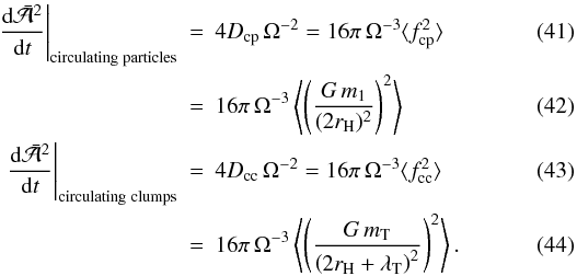 This
is only a crude estimate of the random walk undergone by the moonlet. In reality several
additional effects might also play a role. For example, circulating particles and clumps
are clearly correlated, the gravitational wakes have a large extent in the azimuthal
direction, and particles that spend a long time in the vicinity of the moonlet have more
complex trajectories. Nevertheless, we find that the above estimates are correct up to a
factor 2 for all the simulations that we performed (see below).
This
is only a crude estimate of the random walk undergone by the moonlet. In reality several
additional effects might also play a role. For example, circulating particles and clumps
are clearly correlated, the gravitational wakes have a large extent in the azimuthal
direction, and particles that spend a long time in the vicinity of the moonlet have more
complex trajectories. Nevertheless, we find that the above estimates are correct up to a
factor 2 for all the simulations that we performed (see below).
5.3. Random walk due to particles in horseshoe orbits
Finally, let us calculate the random walk induced by particles on horseshoe orbits.
Particles undergoing horseshoe turns on opposite sides of the planet produce changes of
opposite sign. Encounters with the moonlet are stochastic and therefore the semi-major
axis will undergo a random walk. A single particle with impact parameter
b will change the semi-major axis of the moonlet by
 (45)Analogous
to the analysis in Sect. 5.1, the time evolution of
is then governed by
(45)Analogous
to the analysis in Sect. 5.1, the time evolution of
is then governed by 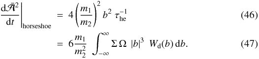 This
equation is identical to Eq. (37) except
for a factor 4, as particles with impact parameter b will leave the
vicinity of the moonlet at − b.
This
equation is identical to Eq. (37) except
for a factor 4, as particles with impact parameter b will leave the
vicinity of the moonlet at − b.
6. Numerical simulations
Initial simulation parameters.
We perform realistic three-dimensional simulations of Saturn’s rings with an embedded moonlet and verify the analytic estimates presented above. The nomenclature and parameters used for the simulations are listed in Table 1. The first column lists the name of the simulation. The second column gives the surface density of the ring. The third gives the moonlet radius. The fourth column gives the timestep. The fifth and sixth columns give the lengths of the main box as measured in the xy-plane and the number of particles used, respectively.
6.1. Methods
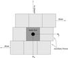 |
Fig. 2 Shearing box, simulating a small patch of a planetary ring system. The particles that leave an auxiliary box in the azimuthal (y) direction re-enter the same box on the other side and get copied into the main box at the corresponding location. All auxiliary boxes are equivalent and there are no curvature terms present in the shearing sheet. |
The gravitational forces are calculated with a Barnes-Hut tree (Barnes & Hut 1986). The numerical scheme is similar to that used by Rein et al. (2010). Additionally, we implemented a symplectic integrator for Hill’s equations (Quinn et al. 2010). This turned out to be beneficial for accurate energy conservation at almost no additional cost when the eccentricity of the moonlet ( ~ 10-8) was small and integrations were undertaken over many hundreds of dynamical timescales.
To speed up the calculations further, we run two coupled simulations in parallel. The first adopts the main box that incorporates a moonlet. The second adopts an auxiliary box which initially has the same number of particles but which does not contain a moonlet. This is taken to be representative of the unperturbed background ring. We describe this setup as enabling us to adopt pseudo shear periodic boundary conditions. We consider the main box together with eight equivalent auxiliary boxes to be stacked as illustrated in Fig. 2. All auxiliary boxes are identical copies whose centres are shifted according to the background shear as in a normal shearing sheet. On account of this motion, auxiliary boxes are removed when their centres are shifted in azimuth by more than 1.5Ly from the centre of the main box and then reinserted in the same orbit on the opposite side of the main box so that the domain under consideration is prevented from shearing out. If a particle in the main box crosses one of its boundaries, it is discarded. If a particle in the auxiliary box crosses one of its boundaries, it is reinserted on the other side of this box, according to normal shear periodic boundary conditions. But in addition it is also copied into the corresponding location in the main box. We describe this procedure as applying pseudo shear periodic boundary conditions.
In a similar calculation, Lewis & Stewart (2009) use a very long box (about 10 times longer than the boxes used in this paper) to ensure that particles are completely randomised between encounters with the moonlet. We are not interested in the long wavelength response that is created by the moonlet. Effects that are most important for the moonlet’s dynamical evolution are found to happen within a few Hill radii. Using the pseudo shear periodic boundary conditions, we ensure that incoming particles are uncorrelated and do not contain prior information about the perturber. This setup speeds up our calculations by more than an order of magnitude.
The gravity acting on a particle in the main box, which also contains the moonlet, is calculated by summing over the particles in the main box and all auxiliary boxes. The gravity acting on a particle in the auxiliary box is calculated the standard way, by using ghost boxes that are identical copies of the auxiliary box. Tests have indicated that our procedure does not introduce unwanted fluctuations in the gravitational forces.
The moonlet is allowed to move freely in the main box. However, to prevent it leaving the computational domain, as soon as the moonlet has left the innermost part (defined as extending one eighth of the box size), all particles are shifted together with the box boundaries, such that the moonlet is returned to the centre of the box. This is possible because the shearing box approximation is invariant with respect to translations in the xy plane (see Eq. (1)).
Collisions between particles are resolved using the instantaneous collision model and a
velocity dependent coefficient of restitution given by Bridges et al. (1984): ![Mathematical equation: \begin{eqnarray} \epsilon(v) &= &\mathrm{min}\left[0.34\cdot \left( \frac{v_\parallel}{10~\mathrm{mm/s}} \right)^{-0.234}, 1\right], \end{eqnarray}](/articles/aa/full_html/2010/16/aa15177-10/aa15177-10-eq168.png) (48)where
v ∥ is the impact speed projected on the axis between the
two particles. The already existing tree structure is reused to search for nearest
neighbours (Rein et al. 2010).
(48)where
v ∥ is the impact speed projected on the axis between the
two particles. The already existing tree structure is reused to search for nearest
neighbours (Rein et al. 2010).
6.2. Initial conditions and tests
Throughout this paper, we use a distribution of particle sizes,
r1, ranging from 1 m to 5 m with a slope of
q = −3. Thus  The density of both the ring particles and the
moonlet is taken to be 4.0kg/m2. This is at the lower end of
what has been assumed reasonable for Saturn’s A ring (Lewis
& Stewart 2009). The moonlet radius is taken to be either 50m or
25m. We found that using a larger ring particle and moonlet density
only leads to more particles being bound to the moonlet. This effectively increases the
mass of the moonlet (or equivalently its Hill radius) and can therefore be easily scaled
to the formalism presented here. Simulating a gravitational aggregate of this kind is
computationally very expensive, as many more collisions have to be resolved each timestep.
The density of both the ring particles and the
moonlet is taken to be 4.0kg/m2. This is at the lower end of
what has been assumed reasonable for Saturn’s A ring (Lewis
& Stewart 2009). The moonlet radius is taken to be either 50m or
25m. We found that using a larger ring particle and moonlet density
only leads to more particles being bound to the moonlet. This effectively increases the
mass of the moonlet (or equivalently its Hill radius) and can therefore be easily scaled
to the formalism presented here. Simulating a gravitational aggregate of this kind is
computationally very expensive, as many more collisions have to be resolved each timestep.
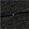 |
Fig. 3 Snapshots of the particle distribution and the moonlet (blue) in simulation EQ40050DTW. The wake is much clearer than in Fig. 4 as the box size is twice as large. |
The initial velocity dispersion of the particles is set to 1mm/s for the x and y components and 0.4mm/s for the z component. The moonlet is placed at a semi-major axis of a = 130000km, corresponding to an orbital period of P = 13.3h. Initially, the moonlet is placed in the centre of the shearing box on a circular orbit.
We run simulations with a variety of moonlet sizes, surface densities, and box sizes. The dimensions of each box, as viewed in the (x,y) plane, are specified in Table 1. Because of the small dispersion velocities, the vertical motion is automatically strongly confined to the mid-plane. After a few orbits, the simulations reach an equilibrium state in which the velocity dispersion of particles does not change anymore.
We ran several tests to ensure that our results are converged. Simulation EQ40050DT uses a ten times longer timestep than simulation EQ40050. Simulations EQ5050DTW, EQ20050DTW, and EQ40050DTW use a box that is twice the size of that used in simulation EQ40050. Therefore, four times more particles are used. No differences in the equilibrium state of the ring particles or in the equilibrium state of the moonlet have been observed in any of those test cases.
A snapshot of the particle distribution in simulation EQ40050DTW is shown in Fig. 3. Snapshots of simulations EQ20025, EQ20050, EQ40025, and EQ40050, which use the smaller box size, are shown in Fig. 4. In all these cases, the length of the wake that is created by the moonlet is much longer than the box size. Nevertheless, the pseudo shear periodic boundary conditions allow us to simulate the evolution of the moonlet accurately.
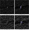 |
Fig. 4 Snapshots of the particle distribution and the moonlet (blue) for different surface densities after 25 orbits. The wake created by the moonlet is much longer than the size of the box and therefore hardly visible in these images. |
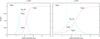 |
Fig. 5 Impact bands for simulation EQ20050 (left) and EQ20025 (right). The vertical lines indicate sharp cutoffs at 1.5rH and 2.5rH. |
7. Results
7.1. Impact bands
The impact band window functions Wa(b), Wb + c(b), and Wd(b) are necessary for estimating the damping timescales and the strength of the excitation. To measure those, each particle that enters the box is labelled with its impact parameter. The possible outcomes are plotted in Fig. 1: (a) being a circulating particle which leaves the box on the opposite side, (b) representing a collision with other ring particles close to the moonlet where the maximum distance from the centre of the moonlet has been taken to be twice the moonlet radius, (c) being a direct collision with the moonlet, and finally (d) showing a horseshoe orbit in which the particle leaves the box on the same side as it entered.
The impact band (b) is considered in addition to the impact band (c) because some ring particles will collide with other ring particles that are (temporarily) bound to the moonlet. Thus, these collisions take part in transferring the energy and momentum to the moonlet. Actually, if the moonlet is simply a rubble pile of ring particles as suggested by Porco et al. (2007), then there might be no solid moonlet core and all collisions are in the impact band (b).
Figure 5 shows the impact bands, normalised to the Hill radius of the moonlet rH for simulations EQ20050 and EQ200252. For comparison, we also plot sharp cutoffs, at 1.5rH and 2.5rH. Our results show no sharp discontinuity because of the velocity dispersion in the ring particles which is ~ 5mm/s. This corresponds to an epicyclic motion of ~ 40m or equivalently ~ 0.8rH and ~ 1.6rH (for r2 = 50m and r2 = 25m, respectively), which explains the cutoff width of approximately one Hill radii. The impact bands are almost independent of the surface density and only depend on the Hill radii and the mean epicyclic amplitude of the ring particles, or, more precisely, on the ratio thereof.
7.2. Eccentricity damping timescale
To measure the eccentricity damping timescale, we first let the ring particles and the
moonlet reach an equilibrium and integrate them for 200 orbits. We then change the
velocity of the moonlet and the ring particles within 2rH. The
new velocity corresponds to an eccentricity of 6 × 10⁻⁷, which is well above
the equilibrium value. We then measure the decay timescale τe
by fitting a function of the form  (49)The
results are given in Table 2. The second column
lists the simulation results. The third and fourth columns list the analytic estimates of
collisional and horseshoe damping timescales, respectively. They are in good agreement
with the estimated damping timescales from Sects. 3.1
and 3.2, showing clearly that the most important
damping process, in every simulation considered here, is indeed through collisional
damping as predicted by comparing Eq. (15)
with Eqs. (19) and (21).
(49)The
results are given in Table 2. The second column
lists the simulation results. The third and fourth columns list the analytic estimates of
collisional and horseshoe damping timescales, respectively. They are in good agreement
with the estimated damping timescales from Sects. 3.1
and 3.2, showing clearly that the most important
damping process, in every simulation considered here, is indeed through collisional
damping as predicted by comparing Eq. (15)
with Eqs. (19) and (21).
7.3. Mean moonlet eccentricity
The mean eccentricity of the moonlet is measured in all simulations after several orbits when the ring particles and the moonlet have reached an equilibrium state. To compare this value with the estimates from Sect. 2, we set Eq. (31) equal to zero and use the analytic damping timescale listed in Table 2. The analytic estimates of the equilibrium eccentricity are calculated for each excitation mechanism separately to disentangle their effects. They are listed in Table 3. The second column lists the simulation results. The third, fourth, and fifth columns list the analytic estimates of the equilibrium eccentricity assuming a single excitation mechanism. The last column lists the analytic estimate of the equilibrium eccentricity summing over all excitation mechanisms. The sixth column lists the analytic estimate for the mean eccentricity using the sum of all excitation mechanisms.
For all simulations, the estimates are correct within a factor of about 2. For low surface densities, the excitation is dominated by individual particle collisions. For higher surface densities, it is dominated by the excitation due to circulating self gravitating clumps (self-gravity wakes). The estimates and their trends are surprisingly accurate, as we have ignored several effects (see below).
7.4. Random walk in semi-major axis
The random walk of the semi-major axis a (or equivalently the centre of
epicyclic motion in the shearing sheet) of the
moonlet in the numerical simulations are measured and compared to the analytic estimates
presented in Sect. 5. We ran one simulation per
parameter set. To get a statistically meaningful expression for the average random walk
after a given time  , we average all pairs of
 and
and
 for which
t − t′ = Δt. In other
words, we assume the system satisfies the Ergodic hypothesis.
for which
t − t′ = Δt. In other
words, we assume the system satisfies the Ergodic hypothesis.
then grows like  and we can fit a simple square root function. This allows us to accurately measure the
average growth in after Δt = 100
orbits by running one simulation for a long time and averaging over time, rather than
running many simulations and performing an ensemble average. The measured values are given
in the second column of Table 4. The second column
lists the simulation results. The third to sixth columns list the analytic estimates of
the change in semi-major axis assuming a single excitation mechanism. The last column
lists the total estimated change in semi-major axis summing over all excitation
mechanisms. These values correspond to the analytic expressions in Eqs. (46), (37), (41), and (44), respectively.
and we can fit a simple square root function. This allows us to accurately measure the
average growth in after Δt = 100
orbits by running one simulation for a long time and averaging over time, rather than
running many simulations and performing an ensemble average. The measured values are given
in the second column of Table 4. The second column
lists the simulation results. The third to sixth columns list the analytic estimates of
the change in semi-major axis assuming a single excitation mechanism. The last column
lists the total estimated change in semi-major axis summing over all excitation
mechanisms. These values correspond to the analytic expressions in Eqs. (46), (37), (41), and (44), respectively.
For low surface densities, the evolution of the random walk is dominated by collisions and the effect of particles on horseshoe orbits. For high surface densities, the main effect comes from the stochastic gravitational force of circulating clumps (self-gravity wakes).
7.5. Long-term evolution and observability
Eccentricity damping timescale τe of the moonlet in units of the orbital period.
Equilibrium eccentricity ⟨ eeq ⟩ of the moonlet.
Change in semi-major axis of the moonlet after 100 orbits,
 .
.
The change in semi-major axis is relatively small at a few tens of metres after 100 orbits ( = 50 days). The change in longitude that corresponds to this is, however, is much larger. We therefore extend the discussion in Rein & Papaloizou (2009), who derive the time evolution of orbital parameters undergoing a random walk, to the time evolution of the mean longitude. This is of special interest in the current situation, because in observations of Saturn’s rings, it is much easier to measure the shift in the longitude of an embedded moonlet than the change in its semi-major axis.
The time derivative of the mean motion is given by
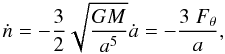 (50)where
Fθ is the time-dependent stochastic force
in the θ (or in shearing sheet coordinates, y)
direction, and we have assumed a nearly circular orbit, e ≪ 1. The mean
longitude is thus given by the double integral
(50)where
Fθ is the time-dependent stochastic force
in the θ (or in shearing sheet coordinates, y)
direction, and we have assumed a nearly circular orbit, e ≪ 1. The mean
longitude is thus given by the double integral 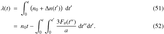 The
root mean square of the difference compared to the unperturbed orbit
(n0) is
The
root mean square of the difference compared to the unperturbed orbit
(n0) is 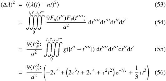 where
g(t) is the auto-correlation function of
Fθ, which has been assumed to be
exponentially decaying with an auto-correlation time τ, thus
g(t) = exp(− | t | /τ).
In the limit t ≫ τ, the above equation simplifies to
where
g(t) is the auto-correlation function of
Fθ, which has been assumed to be
exponentially decaying with an auto-correlation time τ, thus
g(t) = exp(− | t | /τ).
In the limit t ≫ τ, the above equation simplifies to
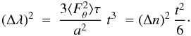 (57)On
a shorter timescale, the other terms in Eq. (56) are important, leading to a linear and oscillatory behaviour. For
uncorrelated noise (e.g. collisions), Eq. (57) is replaced by
(57)On
a shorter timescale, the other terms in Eq. (56) are important, leading to a linear and oscillatory behaviour. For
uncorrelated noise (e.g. collisions), Eq. (57) is replaced by 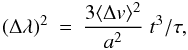 (58)where
⟨ Δv ⟩ is the average velocity change per impulsive event and
τ is taken to be the average time between consecutive events.
(58)where
⟨ Δv ⟩ is the average velocity change per impulsive event and
τ is taken to be the average time between consecutive events.
Instead of a stochastic migration, let us also assume a migration in a laminar disc with
constant migration rate τa, defined by
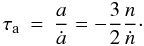 (59)As
above, we can calculate the longitude as a function of time as the following double
integral
(59)As
above, we can calculate the longitude as a function of time as the following double
integral 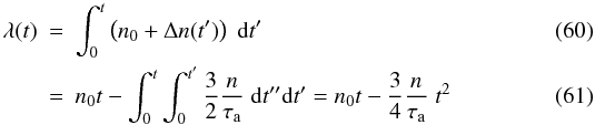 and
thus
and
thus 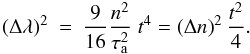 (62)Note
that Eq. (62) is an exact solution,
whereas Eq. (57) is a statistical
quantity, describing the root mean square value in an ensemble average. In the stochastic
and laminar case, (Δλ)2 grows like
~ t3 and ~ t4, respectively.
This behaviour allows a stochastic and laminar migration to be distinguished by observing
Δλ over an extended period of time.
(62)Note
that Eq. (62) is an exact solution,
whereas Eq. (57) is a statistical
quantity, describing the root mean square value in an ensemble average. In the stochastic
and laminar case, (Δλ)2 grows like
~ t3 and ~ t4, respectively.
This behaviour allows a stochastic and laminar migration to be distinguished by observing
Δλ over an extended period of time.
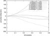 |
Fig. 6 Offset in the azimuthal distance due to the random walk in the semi-major axis a measured in simulations EQ5025, EQ5050, EQ20025, EQ20050, EQ40025 and EQ40050. Individual moonlets may show linear, constant or oscillatory growth. On average, the azimuthal offset grows like t3/2. |
8. Conclusions
In this paper, we have discussed the dynamical response of an embedded moonlet in Saturn’s rings to interactions with ring particles both analytically and by the use of realistic three-dimensional many particle simulations. Both the moonlet and the ring particle density were taken to be 4.0kg/m2. Moonlets of radius 25m and 50m were considered. Particle sizes ranging between 1m and 5m were adopted.
We analytically estimated the eccentricity damping timescale of the moonlet due to both collisions with ring particles and the response of ring particles to gravitational perturbations by the moonlet. We found the effects due to the response of particles on horseshoe and circulating orbits to be negligible. On the other hand, the stochastic impulses applied to the moonlet by circulating particles were found to cause the square of the eccentricity to grow linearly with time as did collisions with particles with non zero velocity dispersion. A balance between excitation and damping processes then leads to an equilibrium moonlet eccentricity.
We also estimated the magnitude of the random walk in the semi-major axis of the moonlet
induced by collisions with individual ring particles and the gravitational interaction with
particles and self-gravity wakes. There is no tendency for the semi-major axis to relax to
any particular value, so that there are no damping terms. The deviation of the semi-major
axis from its value at time t = 0 grows on average as
for
large t.
From our simulations we find that the evolution of the eccentricity is indeed dominated by collisions with ring particles. For high surface densities (more than 200 kg/m2), the effect of self-gravity wakes also becomes important, leading to an increase in the mean steady state eccentricity of the moonlet. When the particle velocity dispersion is larger than ΩrH, we obtain approximate energy equipartition between the moonlet and ring particles as far as epicyclic motion is concerned.
Similarly, the random walk in the semi-major axis was found to be dominated by collisions for low surface densities and by self-gravity wakes for high ones. In addition we have shown that on average, the difference in longitude Δλ of a stochastically forced moonlet grows with time like t3/2 for large t.
The distance travelled within 100 orbits (50 days at a distance of 130 000 km) is, depending on the precise parameters, between 10 m and 100 m. This translates to a shift in longitude of several hundred kilometres. The shift in λ is not necessarily monotonic on short timescales (see Fig. 6). We expect that such a shift should be easily detectable by the Cassini spacecraft. And indeed, the recently published paper by Tiscareno et al. (2010) provides such an observation. These long term observations show that at least one propeller undergoes sustained non-Keplerian orbital motion.
This should be compared with Fig. 6 in this paper, however, the moonlet size differs by a factor four. It can be seen that the observed shift by several hundred kilometres in the azimuthal direction over a year can be easily explained by the mechanisms described in this paper. Future observations and a statistical analysis of the existing observations can further constrain the stochastic nature of the non-Keplerian motion.
There are several effects that have not been included in this study. The analytic discussions in Sects. 3, 4, and 5 do not model the motion of particles correctly when their trajectories take them very close to the moonlet. Material that is temporarily or permanently bound to the moonlet is ignored. The density of both the ring particles and the moonlet are at the lower end of what is assumed to be reasonable (Lewis & Stewart 2009). This has the advantage that for our computational setup only a few particles (with a total mass of less than 10% of the moonlet) are bound to the moonlet at any given time. In a future study, we will extend the discussion presented in this paper to a wider variety of particle sizes, moonlet sizes and densities.
Online material
The Toomre criterion used here was originally derived for a flat gaseous disc. To make use of it, we replace the sound speed by the radial velocity dispersion of the ring particles.
∑ i = a,b,c,dWi ≳ 1 because all particles are shifted from time to time when the moonlet is to far away from the origin (see Sect. 6.1). In this process, particles with the same initial impact parameter might become associated with the more than one impact band.
Acknowledgments
We thank Aurélien Crida for reading an early draft of this paper. Hanno Rein was supported by an Isaac Newton Studentship and St John’s College Cambridge. Simulations were performed on the computational facilities of the Astrophysical Fluid Dynamics Group and on Darwin, the Cambridge University HPC facility.
References
- Barnes, J., & Hut, P. 1986, Nature, 324, 446 [NASA ADS] [CrossRef] [Google Scholar]
- Bridges, F. G., Hatzes, A., & Lin, D. N. C. 1984, Nature, 309, 333 [NASA ADS] [CrossRef] [Google Scholar]
- Crida, A., Papaloizou, J. C. B., Rein, H., Charnoz, S., & Salmon, J. 2010, AJ, 140, 944 [NASA ADS] [CrossRef] [Google Scholar]
- Daisaka, H., Tanaka, H., & Ida, S. 2001, Icarus, 154, 296 [NASA ADS] [CrossRef] [Google Scholar]
- Goldreich, P., & Tremaine, S. 1980, ApJ, 241, 425 [NASA ADS] [CrossRef] [MathSciNet] [Google Scholar]
- Goldreich, P., & Tremaine, S. 1982, ARA&A, 20, 249 [NASA ADS] [CrossRef] [Google Scholar]
- Lewis, M. C., & Stewart, G. R. 2009, Icarus, 199, 387 [NASA ADS] [CrossRef] [Google Scholar]
- Morishima, R., & Salo, H. 2006, Icarus, 181, 272 [NASA ADS] [CrossRef] [Google Scholar]
- Porco, C. C., Thomas, P. C., Weiss, J. W., & Richardson, D. C. 2007, Science, 318, 1602 [NASA ADS] [CrossRef] [PubMed] [Google Scholar]
- Quinn, T., Perrine, R. P., Richardson, D. C., & Barnes, R. 2010, AJ, 139, 803 [NASA ADS] [CrossRef] [Google Scholar]
- Rein H., & Papaloizou, J. C. B. 2009, A&A, 497, 595 [NASA ADS] [CrossRef] [EDP Sciences] [Google Scholar]
- Rein, H., Lesur, G., & Leinhardt, Z. M. 2010, A&A, 511, A69 [NASA ADS] [CrossRef] [EDP Sciences] [Google Scholar]
- Seiß, M., Spahn, F., Sremčević, M., & Salo, H. 2005, Geophys. Res. Lett., 32, 11205 [Google Scholar]
- Spahn F., & Sremčević, M. 2000, A&A, 358, 368 [NASA ADS] [Google Scholar]
- Sremčević, M.,Spahn, F., & Duschl, W. J. 2002, MNRAS, 337, 1139 [Google Scholar]
- Tiscareno, M. S., Burns, J. A., Hedman, M. M., et al. 2006, Nature, 440, 648 [NASA ADS] [CrossRef] [PubMed] [Google Scholar]
- Tiscareno, M. S., Burns, J. A., Hedman, M. M., & Porco, C. C. 2008, AJ, 135, 1083 [Google Scholar]
- Tiscareno, M. S., Burns, J. A., Sremčević, M., et al. 2010, ApJ, 718, L92 [Google Scholar]
Appendix A: Response calculation of particles on horseshoe orbits
A.1. Interaction potential
Due to some finite eccentricity, the moonlet undergoes a small oscillation about the
origin. Its Cartesian coordinates then become (X,Y), with these
considered small in magnitude. The components of the equation of motion for a ring
particle with Cartesian coordinates
(x,y) ≡ r1 are 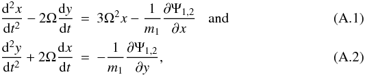 where
the interaction gravitational potential due to the moonlet is
where
the interaction gravitational potential due to the moonlet is
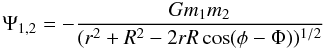 (A.3)with
the cylindrical coordinates of the particle and moonlet being (r,φ) and
(R,Φ), respectively. This may be expanded correct to first order in
R/r in the form
(A.3)with
the cylindrical coordinates of the particle and moonlet being (r,φ) and
(R,Φ), respectively. This may be expanded correct to first order in
R/r in the form 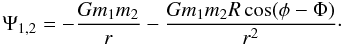 (A.4)The
moonlet undergoes small amplitude epicyclic oscillations such that
X = ℰ2cos(Ωt + ϵ),Y = −2ℰ2sin(Ωt + ϵ)
where e is its small eccentricity and ϵ is an
arbitrary phase. Then Ψ1,2 may be written as
(A.4)The
moonlet undergoes small amplitude epicyclic oscillations such that
X = ℰ2cos(Ωt + ϵ),Y = −2ℰ2sin(Ωt + ϵ)
where e is its small eccentricity and ϵ is an
arbitrary phase. Then Ψ1,2 may be written as
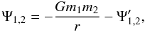 (A.5)where
 (A.6)gives
the part of the lowest order interaction potential associated with the eccentricity of
the moonlet.
(A.6)gives
the part of the lowest order interaction potential associated with the eccentricity of
the moonlet.
We here view the interaction of a ring particle with the moonlet as involving two components. The first term operates when ℰ2 = 0 due to the first term on the right-hand side of Eq. (A.4) and results in standard horseshoe orbits for ring particles induced by a moonlet in circular orbit. The second term, Eq. (A.6), perturbs this motion when ℰ2 is small. We now consider the response of a ring particle undergoing horseshoe motion to this perturbation. In doing so, we make the approximation that the variation in the leading order potential Eq. (A.4) due to the induced ring particle perturbations may be neglected. This is justified by the fact that the response induces epicyclic oscillations of the particle, which are governed by the dominant central potential.
A.2. Response calculation
Setting
x → x + ξx,y → y + ξy,
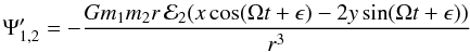
where ξ is the small response displacement induced by Eq. (A.6), and linearising Eqs. (A.1), we obtain the following equations for
the components of ξ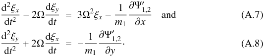 From
these we find a single equation for ξx in
the form
From
these we find a single equation for ξx in
the form  (A.9)When
performing the time integral on the right-hand side of the above, because we are
concerned with a potentially resonant epicyclic response, we only retain the oscillating
part.
(A.9)When
performing the time integral on the right-hand side of the above, because we are
concerned with a potentially resonant epicyclic response, we only retain the oscillating
part.
The solution to Eq. (A.9), which is
such that ξ vanishes in the distant past (t = −∞)
when the particle is far from the moonlet, may be written as
 (A.10)where
 After
the particle has had its closest approach to the moonlet and moves to a large distance
from it, it will have an epicyclic oscillation with amplitude and phase determined by
After
the particle has had its closest approach to the moonlet and moves to a large distance
from it, it will have an epicyclic oscillation with amplitude and phase determined by
 In
evaluating the above we note that, although F vanishes when the
particle is distant from the moonlet at large | t | ,
it also oscillates with the epicyclic angular frequency Ω, which results in a definite
non zero contribution. This is the action of the co-orbital resonance. It is amplified
by the fact that the encounter of the particle with the moonlet in general occurs on a
horseshoe libration timescale that is much longer than Ω-1.
We now consider this unperturbed motion of the ring particles.
In
evaluating the above we note that, although F vanishes when the
particle is distant from the moonlet at large | t | ,
it also oscillates with the epicyclic angular frequency Ω, which results in a definite
non zero contribution. This is the action of the co-orbital resonance. It is amplified
by the fact that the encounter of the particle with the moonlet in general occurs on a
horseshoe libration timescale that is much longer than Ω-1.
We now consider this unperturbed motion of the ring particles.
A.3. Unperturbed horseshoe motion
The equations governing the unperturbed horseshoe motion are Eqs. (A.1) with  (A.15)We
assume that this motion is such that x varies on a timescale that is
much longer than Ω-1 so that we may approximate the first of these equations
as
x = −2/(3Ω)(dy/dt).
Consistent with this, we also neglect x in comparison to
y in Eq. (A.15). From
the second equation we then find that
(A.15)We
assume that this motion is such that x varies on a timescale that is
much longer than Ω-1 so that we may approximate the first of these equations
as
x = −2/(3Ω)(dy/dt).
Consistent with this, we also neglect x in comparison to
y in Eq. (A.15). From
the second equation we then find that  (A.16)which
has a first integral that may be written
(A.16)which
has a first integral that may be written  (A.17)where
as before b is the impact parameter, or the constant value of
| x | at large distances from the moonlet. The value
of y for which the horseshoe turns is then given by
y = y0 = 24Gm2/(9Ω2b2).
At this point we point out that we are free to choose the origin of time
t = 0 such that it coincides with the closest approach at which
y = y0. Then in the approximation we have
adopted, the horseshoe motion is such that y is a symmetric function of
t.
(A.17)where
as before b is the impact parameter, or the constant value of
| x | at large distances from the moonlet. The value
of y for which the horseshoe turns is then given by
y = y0 = 24Gm2/(9Ω2b2).
At this point we point out that we are free to choose the origin of time
t = 0 such that it coincides with the closest approach at which
y = y0. Then in the approximation we have
adopted, the horseshoe motion is such that y is a symmetric function of
t.
A.4. Evaluation of the induced epicyclic amplitude
Using Eqs. (A.6), (A.9), and (A.17), we may evaluate the epicyclic amplitudes from Eq. (A.13). In particular we find
 (A.18)When
evaluating Eq. (A.13), consistent with
our assumption that the epicyclic oscillations are fast, we average over an orbital
period assuming that other quantities in the integrands are fixed, and use Eq. (A.17) to express the integrals with respect
to t as integrals with respect to y. We then find
α∞ = −A‘∞sinϵ
and
(A.18)When
evaluating Eq. (A.13), consistent with
our assumption that the epicyclic oscillations are fast, we average over an orbital
period assuming that other quantities in the integrands are fixed, and use Eq. (A.17) to express the integrals with respect
to t as integrals with respect to y. We then find
α∞ = −A‘∞sinϵ
and
β∞ = −A‘∞cosϵ
where
 (A.19)with
r2 = 8Gm2/(3Ω2y0)(1 − y0/y) + y2.
From this we may write
(A.19)with
r2 = 8Gm2/(3Ω2y0)(1 − y0/y) + y2.
From this we may write 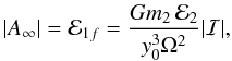 (A.20)where
ℰ1f is the final epicyclic motion of the ring particle and the
dimensionless integral ℐ is given by
(A.20)where
ℰ1f is the final epicyclic motion of the ring particle and the
dimensionless integral ℐ is given by
 (A.21)We
notice that the dimensionless quantity
(A.21)We
notice that the dimensionless quantity  with rH being
the Hill radius of the moonlet. It is related to the impact parameter b
by
η = 2-6(b/rH)6.
Thus for an impact parameter amounting to a few Hill radii, in a very approximate sense,
η is of order unity, y0 is of order
rH, and the induced eccentricity ℰ1f is of
order ℰ2.
with rH being
the Hill radius of the moonlet. It is related to the impact parameter b
by
η = 2-6(b/rH)6.
Thus for an impact parameter amounting to a few Hill radii, in a very approximate sense,
η is of order unity, y0 is of order
rH, and the induced eccentricity ℰ1f is of
order ℰ2.
All Tables
All Figures
|
Fig. 1 Trajectories of ring particles in a frame centred on the moonlet. Particles accumulate near the moonlet and fill its Roche lobe. Particles on trajectories labelled (a) are on circulating orbits. Particles on trajectories labelled (b) collide with other particles in the moonlet’s vicinity. Particles on trajectories labelled (c) collide with the moonlet directly. Particles on trajectories labelled (d) are on horseshoe orbits. Particles on trajectories labelled (e) leave the vicinity of the moonlet. |
| In the text | |
|
Fig. 2 Shearing box, simulating a small patch of a planetary ring system. The particles that leave an auxiliary box in the azimuthal (y) direction re-enter the same box on the other side and get copied into the main box at the corresponding location. All auxiliary boxes are equivalent and there are no curvature terms present in the shearing sheet. |
| In the text | |
|
Fig. 3 Snapshots of the particle distribution and the moonlet (blue) in simulation EQ40050DTW. The wake is much clearer than in Fig. 4 as the box size is twice as large. |
| In the text | |
|
Fig. 4 Snapshots of the particle distribution and the moonlet (blue) for different surface densities after 25 orbits. The wake created by the moonlet is much longer than the size of the box and therefore hardly visible in these images. |
| In the text | |
|
Fig. 5 Impact bands for simulation EQ20050 (left) and EQ20025 (right). The vertical lines indicate sharp cutoffs at 1.5rH and 2.5rH. |
| In the text | |
|
Fig. 6 Offset in the azimuthal distance due to the random walk in the semi-major axis a measured in simulations EQ5025, EQ5050, EQ20025, EQ20050, EQ40025 and EQ40050. Individual moonlets may show linear, constant or oscillatory growth. On average, the azimuthal offset grows like t3/2. |
| In the text | |
Current usage metrics show cumulative count of Article Views (full-text article views including HTML views, PDF and ePub downloads, according to the available data) and Abstracts Views on Vision4Press platform.
Data correspond to usage on the plateform after 2015. The current usage metrics is available 48-96 hours after online publication and is updated daily on week days.
Initial download of the metrics may take a while.