| Issue |
A&A
Volume 524, December 2010
|
|
|---|---|---|
| Article Number | A98 | |
| Number of page(s) | 21 | |
| Section | Stellar structure and evolution | |
| DOI | https://doi.org/10.1051/0004-6361/201014491 | |
| Published online | 25 November 2010 | |
The masses, and the mass discrepancy of O-type stars⋆
1
Scottish Universities Physics Alliance (SUPA), School of Physics and
Astronomy, University of St Andrews,
North Haugh, St Andrews,
Fife
KY16 9SS,
UK
e-mail: This email address is being protected from spambots. You need JavaScript enabled to view it.
2
Armagh Observatory, College Hill, Armagh
BT61 9DG,
UK
e-mail: This email address is being protected from spambots. You need JavaScript enabled to view it.
Received:
23
March
2010
Accepted:
8
September
2010
Abstract
Context. The “mass discrepancy” in massive O stars represents a long-standing problem in stellar astrophysics with far-reaching implications for the chemical and dynamical feedback in galaxies.
Aims. Our goal is to investigate this mass discrepancy by comparing state-of-the-art model masses with model-independent masses determined from eclipsing binaries.
Methods. Using stellar evolution models and a recent calibration of stellar parameters for O-star spectral sub-classes, we present a convenient way to convert observed solar metallicity O star spectral types into model masses, which we subsequently compare to our dynamical mass compilation. We also derive similar conversions for Large and Small Magellanic Cloud metallicities.
Results. We obtain a good agreement between model and dynamical masses, suggesting the long-standing problem of a systematic mass discrepancy problem may have been solved. We also provide error ranges for the model masses, as well as minimal and maximal age estimates for when the model stars are in a given spectral type box.
Key words: binaries: close / binaries: eclipsing / stars: early-type / stars: evolution / stars: formation / stars: fundamental parameters
Appendices and Table 9 are only available in electronic form at http://www.aanda.org
© ESO, 2010
1. Introduction
The most basic parameter of a star is its mass. Knowledge of this most fundamental parameter is of utmost importance for basically all of astrophysics. For massive O stars, reliable mass determinations have turned out to be particularly challenging. For over two decades there has been a “mass discrepancy” where O-star masses derived from evolutionary models (Mevol) were found to be systematically higher than those derived from stellar atmosphere analyses (Mspec) by up to a factor ~2 (Groenewegen & Lamers 1989; Herrero et al. 1992). Even two recent studies still report a significant mass discrepancy for non-enriched O-type stars in the Large Magellanic Cloud (LMC, Mokiem et al. 2007) and the Milky Way (MW, Hohle et al. 2010).
Over the last few decades, four alternative methods to determine O star masses have been developed:
-
evolutionary masses (Mevol)
-
spectroscopic masses (Mspec)
-
wind masses (Mwind)
-
dynamical masses (Mdyn).
In the first method, one places the luminosity (or absolute magnitude) and effective temperature (or colour) in a Hertzsprung-Russell diagram (HRD) and compares the positions of the stars with theoretical stellar evolution models.
The second way comprises the use of stellar spectroscopy: via the Stark broadening in spectral lines, one can derive log g and subsequently the mass Mspec. For O stars, this method is highly complex, because stellar winds have a severe influence on the underlying model atmospheric structure (e.g. Gabler et al. 1989; Hillier 1991).
In the meantime, a third method to determine O star wind masses Mwind had been put forward (Groenewegen & Lamers 1989; Kudritzki et al. 1992). This method employs the radiation-driven theory (e.g. Castor et al. 1975), which relates the terminal wind velocity to the stellar escape velocity. Kudritzki et al. (1992) and Herrero et al. (1992) found good agreement between their spectroscopic and wind masses, and suggested that the evolutionary masses were systematically too large. Although there was indeed no particular reason to expect that evolutionary masses should be correct – given the large number of uncertainties in the underlying physical input (e.g. mass loss, overshooting, rotation, and magnetic effects) – the evolutionary calculations seemed to reproduce the observed O-star properties rather well (Hilditch et al. 1996). Subsequent work by Burkholder et al. (1997), who tried to derive masses from binary dynamics (Mdyn), suggested that the evolutionary masses were at least of the right order of magnitude, thereby challenging the spectroscopic masses, which were significantly lower at the time.
The best argument to trust the spectroscopic masses was their independent agreement with wind masses based on radiation-driven wind theory. This was not always the case as in the 1990s, there was also a systematic discrepancy between mass-loss rates predicted by wind theory and observations (Lamers & Leitherer 1993; Puls et al. 1996). This situation changed when Vink et al. (2000) presented new wind models including multiple-scattering. These models no longer show the systematic discrepancy with empirical rates1. Although the good agreement reached between these new mass-loss predictions and the empirical rates – using the evolutionary rather than the spectroscopic masses – could have been coincidental, the additional compatibility between evolutionary and dynamical masses, resulting in an agreement between three methods, led to the suspicion that it was most likely the spectroscopic masses that were the main culprit for the mass discrepancy.
Lanz et al. (1996) had already suggested that the neglect of line-blanketing could cause Mspec to be underestimated, and subsequent improvements resulted in a new calibration of Galactic O-star parameters by Martins et al. (2005, hereafter MSH05). These state-of-the-art non-local thermodynamic equilibrium (NLTE) models include both mass loss and line-blanketing. In the meantime, the effects of stellar rotation were included in the Geneva evolutionary models (Meynet & Maeder 2003), and below we will indeed confirm that the evolutionary masses now agree with the spectroscopic ones. This should be considered a major triumph for the formidable task of including full Fe line-blanketing in the atmospheric models (e.g. Hillier et al. 2003).
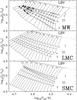 |
Fig. 1 Definitions of the solar metallicity O star spectral types in the luminosity-temperature diagram derived from MSH05 (panel MW), the LMC metallicity (panel LMC) and the SMC metallicity (panel SMC) derived in this work. Panel MW shows the original MSH05 data as crosses and the interpolated 3.5 and 4.5 subclasses as filled circles. Plotted as filled boxes are the extrapolated subtypes 2.5 and 2. The open circles connected by solid lines representes the interpolated grid that defines the L and Teff values for each spectral subtype. The luminosity classes are indicated as Roman numerals (I – supergiants, III – giants and V – dwarfs), while the spectral subtypes are shown by Arabic numerals. The upper limit (dotted line) is given by the hot edge for luminous blue variables (LBV) given in Smith et al. (2004). All interpolations are derived by calculating mean values in linear space. Panel LMC shows the LMC metallicity grid derived from Mokiem et al. (2007) and panel SMC the one for SMC metallicity obtained from Heap et al. (2006). |
Nevertheless, given that both the Geneva evolutionary masses and the MSH05 calibration include the same Vink et al. (2000) mass-loss rates, even an agreement with the wind masses could be a coincidence involving complex model interdependencies, and it is by no means certain they should be correct. It thus remains crucial to check our model masses against model-independent ones.
The only known model-independent masses so far are the dynamically derived ones: Mdyn. This method is only applicable to binary stars. Usually, careful determination of the orbital parameters of a system allows one to obtain the mass ratio of the two stars, as the orbit inclination relative to Earth is generally unknown. Only for eclipsing binaries, the inclination is well-enough constrained to be able to measure absolute stellar masses. Unfortunately, stars eclipsing each other are very rare, and the search for these systems comprises an important endeavor to calibrate and verify evolutionary models. In this paper we provide a compilation of dynamical masses derived from eclipsing binaries. Only very few eclipsing binaries are known that composed of at least one massive star2. All of these are challenging to study because they are distant and, as most or probably all massive stars are born in star clusters (Adams & Myers 2001; Lada & Lada 2003; Allen et al. 2007), in very crowded regions of the sky. Nonetheless, a growing sample of eclipsing O stars is known, and we intend to use these to calibrate a relation between the spectral type of an O star and its present-day mass. Such a relation allows us also to calibrate the masses of O stars that are not part of an eclipsing binary system, i.e. the vast majority!
In Sect. 2 the spectral classification of O stars is discussed, while in Sect. 3 the mass determinations from eclipsing binaries and spectroscopic masses are presented. The results of this study follows in Sect. 4, and a summary is provided in Sect. 5. The stellar evolution models used and our interpolation scheme for additional intermediate model masses is described in Appendix A. Furthermore, a large table is provided in the Appendix B, which shows the spectral type evolution of the different stellar models used (on-line only).
2. Spectral classification of massive stars
Traditionally, O star spectral types are divided into sub-types from O3 to O9, with 0.5 steps (but without the sub-types O3.5 and O4.5). These are observationally defined by the relative strength of the HeI to HeII lines (Conti & Alschuler 1971). Walborn et al. (2002) additionally defined the early O2, O2.5 and O3.5 subtypes, but because the O2 sub-type classification involves the nitrogen (N) sequence rather than the He sequence, these additional sub-types are not (yet) universally accepted. For instance, MSH05 do not use them. For numerical simplicity, we employ the range of sub-types O2 to O9.5, divided into bins of 0.5 width, and with luminosity classes: V (main-sequence), III (giant), and I (supergiant).
Spectral type definitions.
Eclipsing O-star binaries with dynamical mass estimates.
These sub-type–luminosity-classes (from now on spectral type boxes) are defined by six
vertices each, the four corner points and the mean values between the central points of each
box. Each vertice is described by a luminosity and a Teff.
Panel MW of Fig. 1 shows these boxes
for the solar metallicity grid. The central points of the boxes (marked with
crosses) are the new O star spectral type calibrations by MSH05.
Table 1 shows the values of the vertices for the
solar metallicity spectral boxes. As the subtypes O3.5 and O4.5 are not provided by MSH05,
the corresponding values (shown as black dots in Panel A
of Fig. 1) are derived by interpolation
between O3 and O4, and O4 and O5, respectively. For the O2 and O2.5 subtypes, which are not
used by MSH05, their results are extrapolated to these classes (open circles
in Panel A of Fig. 1). The
following fits to their theoretical Teff calibration are used to
define the Teff values for O2 and O2.5 for the three luminosity
classes: 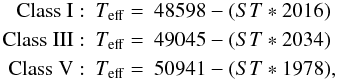 (1)were
ST is the spectral subtype. With these
Teff values and MSH05 Eqs. (3)–(5), the corresponding
luminosities are calculated. The upper limit for the supergiants is set by the empirical hot
edge of the luminous blue variables (LBV) from Smith et al.
(2004)
log 10(LLBVmin) = 2.2056·log 10(Teff) − 3.7737.
If a star is above this line it is regarded to be an LBV. The lower limit is somewhat
arbitrarily set as a parallel line to the luminosity class V, shifted towards higher
temperatures. The border between the O9.5 and B0 subclasses is set by the B0 definitions
from Zorec et al. (2009) for the
Teff and the luminosities from Searle et al. (2008). Whenever a star is earlier than O2, it is designated O2.0
If∗ in the Tables 4 to 7 and 9.
(1)were
ST is the spectral subtype. With these
Teff values and MSH05 Eqs. (3)–(5), the corresponding
luminosities are calculated. The upper limit for the supergiants is set by the empirical hot
edge of the luminous blue variables (LBV) from Smith et al.
(2004)
log 10(LLBVmin) = 2.2056·log 10(Teff) − 3.7737.
If a star is above this line it is regarded to be an LBV. The lower limit is somewhat
arbitrarily set as a parallel line to the luminosity class V, shifted towards higher
temperatures. The border between the O9.5 and B0 subclasses is set by the B0 definitions
from Zorec et al. (2009) for the
Teff and the luminosities from Searle et al. (2008). Whenever a star is earlier than O2, it is designated O2.0
If∗ in the Tables 4 to 7 and 9.
Naturally, such a scheme is not to be expected to be in full compliance with how the spectral indices for O stars change with Teff. To compensate for this, a general error of 1000 K is assumed for all Teff values used.
About one third of the stars with dynamical mass estimates (Table 2) are located in the LMC. This dwarf galaxy has a considerably lower
metallicity than solar (zLMC ≈ 0.008, van den Bergh 2000) and therefore solar metallicity spectral definitions
and evolutionary models might not represent these stars well. Especially the
Teff scale of LMC metallicity stars is well above solar
metallicity ones (Evans 2009). As a comprehensive
study of O type spectral classes like MSH05 does not exist for LMC metallicity stars, the
sample of LMC O and early B-type stars of Mokiem et al.
(2007) is used to fit the following relations between
Teff and log 10(L) for LMC
metallicity O stars. 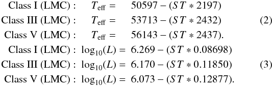 The
resulting spectral type grid is shown in Table 1 and
as Panel LMC of Fig. 1.
The
resulting spectral type grid is shown in Table 1 and
as Panel LMC of Fig. 1.
While there are no eclipsing binaries in Table 2
with SMC metallicities (zSMC ≈ 0.004, van den Bergh 2000), a
recent Teff calibration for O stars in the SMC does exist (Heap et al. 2006). Their data are used to derive the
following Teff and luminosity relations in dependence of the
spectral subtype. 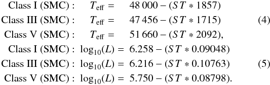 Like
in the other two cases the spectral type grid is included in Table 1 and it is shown in Panel SMC of Fig. 1. As is visible in Fig. 1 and Table 1, the SMC
Teff grid is shifted to lower temperatures
compared to the LMC grid. The reason for this is non-trivial, and deserves a thorough
analysis using SMC metallicity NLTE atmospheres, which is beyond the scope of this paper.
Note that the Heap et al. (2006) sample only includes
one star with a spectral type earlier than O4. This star is not included in the relations,
but the relations are used from O2 to O9.5.
Like
in the other two cases the spectral type grid is included in Table 1 and it is shown in Panel SMC of Fig. 1. As is visible in Fig. 1 and Table 1, the SMC
Teff grid is shifted to lower temperatures
compared to the LMC grid. The reason for this is non-trivial, and deserves a thorough
analysis using SMC metallicity NLTE atmospheres, which is beyond the scope of this paper.
Note that the Heap et al. (2006) sample only includes
one star with a spectral type earlier than O4. This star is not included in the relations,
but the relations are used from O2 to O9.5.
In order to assign a certain spectral subtype and luminosity class to a specific evolutionary point in time, stellar evolution models from Meynet & Maeder (2003) (see also Appendix A) are followed throughout the Teff-L-diagram. This is visualized in Fig. 2, where the luminosity- and Teff-evolution for six rotating as well as non-rotating stellar models from 20 to 120 M⊙ (Meynet & Maeder 2003) are plotted (rotating models as dashed lines and non-rotating ones as dotted lines). In this figure, only the part of the evolution before the Wolf-Rayet (WR) stage is depicted. Objects that are still assumed to be core hydrogen are classified as WNL stars (Hamann et al. 2006). However, we note that the WNL classification is only used in Appendix B. The present-day mass of a model during its evolution through a spectral subclass is from now on referred to as evolutionary mass (Mevol).
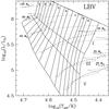 |
Fig. 2 Similar as panel A of Fig. 1, but only the spectral subtype boxes are shown as a grid of solid lines. The dashed lines are rotating and the dotted lines non-rotating solar metallicity stellar evolutionary tracks by Meynet & Maeder (2003) with initial masses as indicated in the figure. Only evolutionary phases before the Wolf-Rayet stage are plotted. |
Table 4 shows the new spectral type mass conversion, based on solar metallicity rotating evolutionary models from 10 to 120 M⊙ (Meynet & Maeder 2003). The rotating models have initial rotational velocities (vrot ini) of 300 km s-1, which results in vrot during the Main-Sequence evolution of 180 to 240 km s-1. These velocities are within the range observed for O stars (Mokiem et al. 2006). A table with non-rotating models is provided as Table 5. As the Meynet & Maeder (2003) models only provide a limited mass resolution, a special interpolation routine (described in detail in Appendix A) is deployed in order to provide a mass resolution down to 1 M⊙. For LMC metallicity Meynet & Maeder (2005) provide only four models (30, 40, 60 and 120 M⊙, all rotating with 300 km s-1), two additional models (15 and 20 M⊙) are taken from the Padova group (Bertelli et al. 2009). The resulting spectral type mass conversion for LMC metallicity stars is shown in Table 6. For SMC metallicities, Meynet & Maeder (2003) only include three (all rotating) models (40, 60 and 120 M⊙). Again, two models are added here (15 and 20 M⊙) from Bertelli et al. (2009) in order to derive a spectral type mass conversion (Table 7).
O-star with spectroscopic mass estimates.
The masses shown in the Tables 4 to 7 are all weighted by the duration of the models in each spectral class. The errors are assigned by using the most- and least-massive model entering the spectral class. As mentioned before, each spectral class has an assumed error in Teff of 1000 K. The minimal and maximal start and end ages give the range of possible ages for the stars in a spectral-class box. The advantage of using this method is the consistent application of observational constraints for the different evolutionary phases on one set of stellar evolution models. This allows one to place more constraints for the stars in a certain spectral class on the range of their initial and present-day masses.
A number of other mass estimates for spectral types exist in the literature, e.g. Vacca et al. (1996) and Hanson et al. (1997), but only the most recent one by MSH05 is used here. These
models provide spectroscopic stellar masses that are derived from the stellar luminosity,
L, and Teff of NLTE stellar atmosphere models
through  (6)where
G equals Newton’s gravitational constant, and g is the
gravitational acceleration of the star at radius R:
(6)where
G equals Newton’s gravitational constant, and g is the
gravitational acceleration of the star at radius R:  (7)where
σR is the Stefan-Boltzmann constant. Martins et al. (2005) provide two mass estimates, one for a theoretical
Teff calibration (mMSH1) and one
for an observational Teff calibration
(mMSH2).
(7)where
σR is the Stefan-Boltzmann constant. Martins et al. (2005) provide two mass estimates, one for a theoretical
Teff calibration (mMSH1) and one
for an observational Teff calibration
(mMSH2).
Instead of using spectral type calibrations, a more direct way to derive spectroscopic masses is by carefully fitting model atmospheres to high-resolution spectra, where both g, and Teff are determined simultaneously (see for example Repolust et al. 2004). Together with its absolute magnitude it is possible to arrive at a mass using Eqs. (6) and (7). A sample of spectroscopic masses derived with this method will also be compared with dynamical and model masses.
2.1. Limitations
Although the results presented here cover a large parameter space, they involve some caveats. First of all, both the employed Meynet & Maeder (2003) stellar evolution models, as well as the MSH05 stellar atmospheres, which define our spectral classes, only cover solar metallicity (z = 0.02). Metallicity is known to have a very strong influence on the evolution and atmospheres of (O) stars via their metallicity-dependent winds. The newly developed spectral type definitions for LMC and SMC metallicities are a first step to loosen these limitations, but are not as thoroughly based as the MSH05 work for solar metallicity.
Table 9 shows the spectral evolution of a series of massive stellar models of different metallicities (z = 0.004, 0.008, 0.02 and 0.04, Meynet & Maeder 2003, 2005) using the spectral type definitions in Table 1. While these spectral type definitions are based on solar metallicity atmospheres or empirical Teff calibrations (for z = 0.008 and z = 0.004), considerable differences in the evolution are noticeable.
Another relevant aspect for the evolution of massive stars concerns binary evolution. Because many (if not most) massive stars are part of a binary system, often with considerable secondary masses (Preibisch et al. 1999; Apai et al. 2007; Kobulnicky & Fryer 2007; Ritchie et al. 2009; Weidner et al. 2009; Sana et al. 2010), they could be capable of influencing each other’s evolution in a profound manner. Because all observations presented in Table 2 involve eclipsing binaries, all the objects must form tight pairs with reasonably large stars, and therefore binary evolution is bound to be important, but it is a non-trivial matter to account for it.
As was mentioned in the introduction, an additional potential prime source for errors in the mass determination concerns the atmosphere and wind parameters, as well as the mass-loss prescription employed in the evolutionary models.
3. Dynamical masses of eclipsing binaries
In recent years, observational techniques allowed us to measure masses of very massive stars directly by observing the orbits of massive eclipsing binaries. In Table 2 the dynamical mass estimates for 33 very massive stars are listed. The majority of the stars (22) are from a compilation by Gies (2003), who provides three lists with massive binaries from the literature. His first list shows detached systems, the second one non-eclipsing binaries (with lower mass limits only) and the third systems, which are either dynamically evolved (semi-detached or contact systems) or contain giants or supergiants. All but two systems from the first list are included in Table 2 as are three systems form the third list, two of them are given as being before the interaction stage and the supergiant V729 Cyg. The systems with lower limits only and the ones which are dynamically evolved are not suitable for the current study and are therefore not included. The remaining eclipsing binaries except one are from literature published after the Gies (2003) list, but which contain the necessary data for this study. The exception is WR22 B, which is not covered in Gies (2003) because the primary is a Wolf-Rayet star.
The dynamical masses from Table 2 involve present-day masses instead of initial masses. This is accounted for by not only comparing the evolving parameters with the luminosity and Teff grid, but by simultaneously keeping track of the initial mass. Therefore, in Table 4 the initial stellar mass for a spectral type is given as well as the possible minimal and maximal mass when the stars enter and leave the respective spectral type. Additionally, the minimal and maximal age is given when the models enter and leave a spectral type.
In addition to dynamical mass determinations, several spectroscopic masses exist for O-type stars. Table 3 shows a compilation of these spectroscopic masses taken from Repolust et al. (2004), besides the MSH05 masses and the evolutionary masses presented in this work.
4. Results and discussion
The Tables 4 and 5 show the determined initial masses as well as the mean, minimal, and maximal present-day masses according to the Meynet & Maeder (2003) rotating (300 km s-1) and non-rotating stellar evolution models, and the MSH05 O star spectral type definition. Tables 6 and 7 show the same for LMC and SMC metallicities, respectively. The errors shown for the mass determination are the lowest mass and maximum mass models that pass through the spectral type. They also include an error margin of ± 1000 K for the MSH05 spectral type definitions. The differences in the supergiant mass errors from one subtype to the next have two main reasons. Spectral types later than O 6.5 I are reached during stellar evolution from the hot end by more massive stars and the cold end by less massive stars. This results in a larger range of possible masses. Also, the subtypes are not of the same area in the L-Teff -space (see Fig. 1). Therefore, some subtypes simply have a higher probability to be encountered by the model tracks. It would be possible to reduce these errors by introducing more luminosity classes, like II, Ia and Ib. But no MSH05 definitions for these classes presently exist.
Furthermore, the table shows the mean time the models spend in each spectral type box. Again, the errors are defined by the lowest and most-massive model passing through the spectral type box, including a ± 1000 K uncertainty for the spectral type definitions. Note that the Meynet & Maeder (2003) models show considerable jumps in Teff and luminosity when the stars enter the Wolf-Rayet phase. These extremely fast crossings ( < 50 000 years) through the HR-Diagram are not included in the tables.
Theoretical masses for O stars from rotating stellar models.
Theoretical masses for O stars from non-rotating stellar models.
Theoretical masses for O stars from rotating LMC (z = 0.008) stellar models.
Theoretical masses for O stars from rotating SMC (z = 0.004) stellar models.
The newly arrived spectral-type-mass relation, as arrived in Sect. 2, is now compared with the dynamical (Table 2) and literature spectroscopic (Table 3) mass estimates from Sect. 3.
4.1. Comparison with dynamical masses
In Fig. 3 the results of the MSH05 and the present-day mass estimates are compared with dynamical mass estimates for massive stars from the literature as shown in Table 2. Inspecting the mass estimates, a very large spread is noticeable.
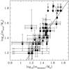 |
Fig. 3 Comparison of the different mass estimates with dynamically determined stellar masses. The solid line marks a one-to-one correspondence between model and dynamical mass. Open circles show the masses for the MSH05 theoretical O star Teff scale, closed circles for the MSH05 observational temperature scale and open boxes mark the mean masses derived in this work. |
The results of a linear correlation analysis for all stars in the sample are shown in Table 8. For each sample, the slope and offset of a best-fitting linear relation are given together with the correlation coefficients. The “MSH1” column provides the mass estimates from MSH05 using the theoretical Teff scale, whilst “MSH2” gives the results from their observational Teff scale. “ini”, “evol”, “start” and “end” are the results arrived at here, with “ini” marking the results for initial masses of the models, “start” the evolved mass when a star enters a spectral type and “end” the one when he leaves it. “Evol” is the mean mass computed from mstart and mend. With an offset very close to 0, a slope of nearly 1, and a correlation coefficient of ~0.9, the MSH05 mass estimates agree very well with the dynamical masses of the sample. Furthermore, the minimal, maximal, and evolutionary present-day masses, which are calibrated on the theoretical Teff scale of MSH05, agree very well with the observed dynamical masses. The offsets are quite close to 0 and slopes similarly close to 1, whilst the correlation coefficients are ~0.9 too. The present-day dynamical masses are therefore quite well reproduced by the models. Note that the errors for the MSH05 based fits are always smaller than the fits with the here-derived values. This is because the MSH05 values involve no errors, and the fit only contains errors in the dynamical masses. The values derived here also have their own error estimate.
In Figs. 4–6 the dynamical masses from Table 2 (open circles) are shown together with the present-day mass range (mstart to mend) for the models (shaded region), for the supergiants (Fig. 4), giants (Fig. 5) and dwarfs (Fig. 6). Evidently, most of the dynamical measurements agree well with the models within the error bars. For supergiants and giants the mass ranges for different metallicities are nearly indistinguishable. Only the non-rotating evolutionary models stand out in the case of the supergiants. Because the dependence of mass loss on rotation is not understood very well, this discrepancy is likely very dependent on the assumptions in the stellar evolutionary code. For dwarf stars only the SMC metallicity mass ranges differ visibly from the solar and LMC estimates. Somewhat surprisingly, the early-type SMC dwarfs seem to have lower masses than their MW and LMC cousins, according to the models and definitions used here. This is almost certainly because of the earlier mentioned perhaps unexpected fact that the Heap et al. (2006) SMC O stars result in a lower Teff scale for O stars than for LMC objects.
Interestingly, all but two of the (dwarf) stars located in the LMC (en-circled circles in Fig. 6) lie below the here derived solar and LMC metallicity evolutionary mass ranges, independent of rotation and metallicity. Only the allowed mass range for SMC metallicity covers these stars.
This might be because of binary stellar evolution because it is more difficult to access if the stars are detached or not in the LMC. The lower metallicity of the LMC might also not be accounted for correctly either in the evolutionary models or in the atmosphere models. The large distance to these stars compared to the rest of the sample might also influence the observed values. However, removing these nine stars from the already small sample of only 30 stars would strongly reduce its significance.
In one case (V1182 Aql A) the initial mass is slightly above the dynamical mass for its spectral type, even when considering the uncertainties in the observational and model mass determination. This might be caused by a somewhat optimistic observational error ( ± 0.6 M⊙) or can be because of binary stellar evolution effects such as mass transfer, or excess irradiation of one stellar hemisphere in tidally locked configurations.
Correlation function values.
4.2. Comparison with spectroscopic masses
Spectroscopic mass determinations are the only other empirical method to derive stellar masses for single stars and non-eclipsing binaries. The hot and usually rapidly-rotating O stars have very broad spectral features, which often result in large error bars from the line-fitting techniques used to fit model spectra to observations. The literature spectroscopic mass values from Repolust et al. (2004) are shown in Table 3 and are also plotted in Figs. 4 to 6 as filled circles. The spread seems to be somewhat larger than the spread of the dynamical mass estimates and it should be noted that several (3 out of 21) of the spectroscopic measurements are so far outside the predictions that the error bars do not overlap. Two of these three stars are giants (HD190864 and HD193682) and one is a dwarf (HD217086). Reassuringly, all supergiants (Fig. 4) overlap at least with their error bars with the model predictions, and apart from the mentioned exceptions all giants and dwarfs, too.
The large spread and the three outlying stars might be because of the generally much larger errors of the spectroscopic masses determinations compared to dynamical ones. Heap et al. (2006) find in their study of SMC stars that the mass discrepancy is reduced but not eliminated when using NLTE line-blanketed model atmospheres. They suggest that the remaining difference is actually a signature of fast rotation that would lower the apparent surface gravity. As also indicated in Table 3, some of the stars are known binaries and two runaway stars are also included in the sample, though theses stars agree reasonably well with the models. For such objects binary stellar evolution could have strongly influenced the present-day mass, and/or spectrum of the star. Nonetheless, the evolutionary model based spectral-type–mass-relation derived here agrees with dynamical as well as spectroscopic mass estimates, suggesting the systematic mass-discrepancy problem might be solved.
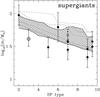 |
Fig. 4 Comparison of the dynamical (open circles) and spectroscopic (filled circles) mass measurements for luminosity class I objects (supergiants) with the evolutionary masses. The shaded region between the solid lines shows the full range (mstart to mend) of evolutionary masses for the rotating solar metallicity models. The dashed lines mark the upper and lower mass ranges for the non-rotating solar metallicity models, while the dotted lines bracket the possible masses for the rotating LMC metallicity models and the dashed-dotted lines enclose the SMC metallicity models. Double encircled objects are located in the LMC. |
5. Summary and conclusions
With the spectral type definition of MSH05, a relation between O star spectral type and its mass and age was derived for solar metallicity stars. This was achieved by taking stellar evolution models (Meynet & Maeder 2003) and comparing their output luminosities and Teff with the MSH05 spectral type definitions. With the Mokiem et al. (2007) study of O stars in the LMC, the Heap et al. (2006) data for SMC O stars and evolutionary tracks by Meynet & Maeder (2005) and Bertelli et al. (2009), similar spectral-type–mass-relations were derived for LMC and SMC metallicity. The resulting mass versus spectral-type relation agrees well with dynamical as well as spectroscopic mass measurements from the literature for MW and LMC main-sequence stars. For SMC stars, giants and supergiants too few or no dynamical mass estimates are available for an in-depth comparison.
Tables 4 and 5 provide easy access to the mass estimates for a given spectral type based on rotating (Table 4) and non-rotating (Table 5) solar metallicity O star models. Tables 6 and 7 provide the same for LMC and SMC metallicity.
Furthermore, the evolution of individual stellar models (Meynet & Maeder 2003, 2005; Bertelli et al. 2009) through the different spectral types are given in Appendix B. For the z = 0.02 and 0.04 the MSH05 solar metallicity definitions of spectral types are used, while for z = 0.008 the LMC ones and for z = 0.004 the SMC ones.
The new calibration of O star spectral types presented here with stellar evolution models provides a valuable new tool to derive O star masses, including initial and present-day masses, and includes an estimate of the errors. Furthermore, the minimal and maximal start and end ages for a given spectral class provide relevant information for statistical studies of roughly solar-metallicity young stellar populations. The relation derived here between spectral type and evolutionary mass agrees very well with dynamical as well as spectroscopic mass estimates for O stars from the literature and is therefore quite robust. No systematic discrepancy between dynamical, model and spectroscopic mass estimates could be found.
Because there are still considerable error margins in the new calibration, more observational and theoretical effort is necessary in order to improve on these. Larger samples of O stars with homogeneously derived parameters and larger sets of evolutionary models with a broader range of initial conditions (vrot, metallicity, magnetic fields and, especially initial mass) would help to improve the calibration. Interestingly, seven out of nine stars located in the LMC (en-circled circles in Figs. 4 and 6) are below or at the lower end of the predicted evolutionary mass range. Even when considering an LMC metallicity luminosity-Teff grid and evolutionary models (dashed lines in Figs. 4 to 6). These systematically lower dynamic masses could have several reasons. The influence of metallicity on the atmosphere and stellar models might be underestimated or these stars could be undetected contact systems instead of detached systems. Or stars earlier than O6 in the LMC are systematically misclassified and should all be shifted by one spectral subtype towards later types.
An additional startling fact are the low Teff of the spectral type definitions for SMC metallicities and the resulting lower masses for early SMC O stars. This is probably because of the lack of early O stars in the Heap et al. (2006) SMC study used here to calibrate the SMC spectral types. Yet these lower masses fit the eclipsing LMC (!) early O stars much better than the hot LMC spectral type definitions.
The other major source for uncertainties is massive binary evolution. It is a major obstacle, especially for giant and supergiant systems with dynamical mass estimates. These are generally short-period systems and the increasing radii of giants and supergiants during their evolution make mass transfer highly likely. Whilst the modelling of the relevant processes has significantly improved in recent years (Eldridge et al. 2008; Langer et al. 2008; de Mink et al. 2009; Song et al. 2009; van Rensbergen et al. 2010), the huge parameter space of hitherto unknown initial conditions (mass ratio, eccentricity, period, orbital inclination) and the possibility of reaching the same final state from different initial ones makes a correction for binary stellar evolutionary effects most challenging.
Given the internal consistency of the three model-dependent mass determinations (Mevol, Mspec and Mwind) it would be tempting to conclude that the basic properties of main-sequence O-type stars are now well understood. However, we point out that all that wind masses, the MSH05 calibrations, and the rotating Geneva stellar tracks all employ the same underlying mass-loss prescriptions of Vink et al. (2000), and these have recently been suggested to be too high (e.g. Fullerton et al. 2006) as a result of wind clumping. If calls for a fundamental downwards revision for O-star mass-loss rates were proven to be correct, this would undoubtedly result in the creation of new mass discrepancies. It may therefore be considered highly significant that current model masses seem to be backed up by model-independent dynamical masses – boosting confidence in our basic knowledge of the physical parameters, such as its mass-loss rate, and the modelling of the atmospheres and evolution of O-type stars.
Ironically it appears that the O-stars are currently better understood than the adjacent spectral type B-type stars, for which Cantiello et al. (2009, see their Fig. 10; with data from Trundle et al. 2007 and Hunter et al. 2008 showed a highly significant mass discrepancy, with evolutionary masses up to a factor three larger than spectroscopic ones.
Online material
Appendix A: Stellar evolution
The evolution of stars used in this work is based on the stellar evolution models for solar and non-solar metallicity, rotating with 300 km s-1 and non-rotating by Meynet & Maeder (2003) and Meynet & Maeder (2005) and each two models with LMC and SMC metallicity (15 and 20 M⊙) by Bertelli et al. (2009). Model tracks are only provided for stars with 9, 12, 15, 20, 25, 40, 60, 85 and 120 M⊙ for solar metallicity and even fewer for non-solar metallicity. As the lifetime of the stars and their respective evolutionary stages are dependent on the mass of the star, it is not possible to linearly interpolate between the track of a 40 and a 60 M⊙ star in order to get, for example, a 50 M⊙ star. Therefore, a special interpolation routine is employed here. The model tracks immediately above and below the target mass are normalized to their individual lifetimes (the point when the star becomes a neutron star or a black hole). Then the two normalized tracks are interpolated linearly to the target mass. The resulting track is then multiplied with the lifetime for the targeted star. This lifetime is linearly interpolated from the lifetime of the two input models.
Figure A.1 shows the stellar evolution of a 85 M⊙ and a 120 M⊙ star with time from Meynet & Maeder (2003) for several stellar parameters (luminosity, radius, mass, Teff) together with an interpolated track of a 100 M⊙ star.
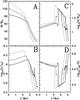 |
Fig. A.1 Panel A: mass evolution over 4 Myr for a 85 M⊙ (solid line) and a 120 M⊙ star (dotted line) from literature data (Meynet & Maeder 2003). The dashed line shows a 100 M⊙ star interpolated from the two models. Panel B: luminosity evolution over 4 Myr for the same three stars as in the panel A. Panel C: radius evolution over 4 Myr for the same three stars as in panel A. Panel D: effective temperature evolution over 4 Myr for the same three stars as in panel A. |
Appendix B: Spectral-type-stellar evolution tables
The following Table 9 shows the different spectral types that stellar evolution models reach during their lifetime. It uses solar metallicity (Meynet & Maeder 2003) and non-solar metallicities (Meynet & Maeder 2005) and rotating (vrot,initial = 300 km s-1) and non-rotating tracks between 20 and 120 M⊙. In this table are also shown evolutionary phases that go beyond the O spectral type used in the current work. Below we describe how these additional phases are classified. As the surface abundances for
several species (H, He, C, N, O, Ne and Al) are also given in the models, it is possible to assign the beginning of the hydrogen-rich Wolf-Rayet phase (WNL) as soon the surface hydrogen abundance is below 60% (Hamann et al. 2006) and the helium-rich Wolf-Rayet phase (WNE) is given when the surface abundance of hydrogen is below 10-4. Later on, stars are designated as carbon-rich Wolf-Rayet stars (WC) when helium starts to be depleted on the surface and the carbon abundance rises above 10-4. Exceptions from this scheme are made when the stars enter the Luminous Blue Variable (LBV), Yellow Hyper-Giant (YHG), Yellow Giant (YG), Blue Supergiant (BSG) or Red Supergiant (RSG) phases. The hot end of the LBVs is defined by log 10(LLBV hot) = 2.2056·log 10(Teff) − 3.7737 and on the cool edge by TLBV cool = 7500 K with a lower limit of log 10(L/L⊙) = 5.3 (Smith et al. 2004). YHGs lie between 4500 to 7500 K and log 10(L/L⊙) ≥ 5.3 (Smith et al. 2004). Models that evolve between 4500 to 7500 K, but have log 10(L/L⊙) < 5.3, are named YGs. The BSGs are stars that are too cold for the O9.5 III or the O9.5 I types, but that are still below the LBV limit and hotter than YHGs. And finally, RSGs are stars colder than 4500 K and log 10(L) ≥ 3.55log 10(L/L⊙) (Levesque 2010).
The evolutionary sequence for solar metallicity roughly agrees with the currently used observational sequence by e.g. Crowther (2007):
-
Minitial > 75 M⊙: O → WNL → LBV → WNE → WC → SNIc,
-
Minitial = 40–75 M⊙: O → LBV → WNE → WC → SNIc,
-
Minitial = 25–40 M⊙: O → LBV/RSG → WNE → SNIb.
Where SNIb and SNIc are supernovae type Ib and Ic, although it has recently been suggested that LBVs could explode early (Kotak & Vink 2006; Gal-Yam & Leonard 2009), which would significantly alter the later evolutionary phases of these types of schemes.
Spectral type evolution of stellar models.
Although it is currently debated whether the absolute values of these mass-loss rates are of the right order of magnitude. Some recent studies have called for a fundamental reduction in O-star mass-loss rates as a result of wind clumping (Bouret et al. 2005; Fullerton et al. 2006).
For the context of this publication massive stars are solely O stars that are thought to have masses of about 16 M⊙ and larger.
Acknowledgments
C.W. is happy to thank Jan Pflamm-Altenburg, Jim Dale, Nick Moeckel and Ian Bonnell for helpful discussions. This work made use of the Simbad web based database. This work was financially supported by the CONSTELLATION European Commission Marie Curie Research Training Network (MRTN-CT-2006-035890).
References
- Adams, F. C., & Myers, P. C. 2001, ApJ, 553, 744 [NASA ADS] [CrossRef] [Google Scholar]
- Allen, L., Megeath, S. T., Gutermuth, R., et al. 2007, in Protostars and Planets V, ed. B. Reipurth, D. Jewitt, & K. Keil, 361 [Google Scholar]
- Apai, D., Bik, A., Kaper, L., Henning, T., & Zinnecker, H. 2007, ApJ, 655, 484 [NASA ADS] [CrossRef] [Google Scholar]
- Bertelli, G., Nasi, E., Girardi, L., & Marigo, P. 2009, A&A, 508, 355 [NASA ADS] [CrossRef] [EDP Sciences] [Google Scholar]
- Bonanos, A. Z. 2009, ApJ, 691, 407 [NASA ADS] [CrossRef] [Google Scholar]
- Bouret, J., Lanz, T., & Hillier, D. J. 2005, A&A, 438, 301 [NASA ADS] [CrossRef] [EDP Sciences] [Google Scholar]
- Burkholder, V., Massey, P., & Morrell, N. 1997, ApJ, 490, 328 [NASA ADS] [CrossRef] [Google Scholar]
- Cantiello, M., Langer, N., Brott, I., et al. 2009, A&A, 499, 279 [NASA ADS] [CrossRef] [EDP Sciences] [Google Scholar]
- Castor, J. I., Abbott, D. C., & Klein, R. I. 1975, ApJ, 195, 157 [NASA ADS] [CrossRef] [Google Scholar]
- Conti, P. S., & Alschuler, W. R. 1971, ApJ, 170, 325 [NASA ADS] [CrossRef] [Google Scholar]
- Crowther, P. A. 2007, ARA&A, 45, 177 [NASA ADS] [CrossRef] [Google Scholar]
- de Mink, S. E., Cantiello, M., Langer, N., et al. 2009, A&A, 497, 243 [NASA ADS] [CrossRef] [EDP Sciences] [Google Scholar]
- Eldridge, J. J., Izzard, R. G., & Tout, C. A. 2008, MNRAS, 384, 1109 [NASA ADS] [CrossRef] [Google Scholar]
- Evans, C. J. 2009, in The Magellanic System: Stars, Gas, and Galaxies, ed. J. T. van Loon & J. M. Oliveira, IAU Symp., 256, 325 [Google Scholar]
- Fernández Lajús, E., & Niemela, V. S. 2006, MNRAS, 367, 1709 [NASA ADS] [CrossRef] [Google Scholar]
- Fullerton, A. W., Massa, D. L., & Prinja, R. K. 2006, ApJ, 637, 1025 [NASA ADS] [CrossRef] [Google Scholar]
- Gabler, R., Gabler, A., Kudritzki, R. P., Puls, J., & Pauldrach, A. 1989, A&A, 226, 162 [NASA ADS] [Google Scholar]
- Gal-Yam, A., & Leonard, D. C. 2009, Nature, 458, 865 [NASA ADS] [CrossRef] [PubMed] [Google Scholar]
- Gies, D. R. 2003, in A Massive Star Odyssey: From Main Sequence to Supernova, ed. K. van der Hucht, A. Herrero, & C. Esteban, IAU Symp., 212, 91 [Google Scholar]
- Groenewegen, M. A. T., & Lamers, H. J. G. L. M. 1989, A&AS, 79, 359 [NASA ADS] [Google Scholar]
- Hamann, W.-R., Gräfener, G., & Liermann, A. 2006, A&A, 457, 1015 [NASA ADS] [CrossRef] [EDP Sciences] [Google Scholar]
- Hanson, M. M., Howarth, I. D., & Conti, P. S. 1997, ApJ, 489, 698 [NASA ADS] [CrossRef] [Google Scholar]
- Heap, S. R., Lanz, T., & Hubeny, I. 2006, ApJ, 638, 409 [NASA ADS] [CrossRef] [Google Scholar]
- Herrero, A., Kudritzki, R. P., Vilchez, J. M., et al. 1992, A&A, 261, 209 [NASA ADS] [Google Scholar]
- Hilditch, R. W., Harries, T. J., & Bell, S. A. 1996, A&A, 314, 165 [NASA ADS] [Google Scholar]
- Hillier, D. J. 1991, A&A, 247, 455 [NASA ADS] [Google Scholar]
- Hillier, D. J., Lanz, T., Heap, S. R., et al. 2003, ApJ, 588, 1039 [NASA ADS] [CrossRef] [Google Scholar]
- Hohle, M. M., Neuhäuser, R., & Schutz, B. F. 2010, Astron. Nachr., 331, 349 [NASA ADS] [CrossRef] [Google Scholar]
- Hunter, I., Lennon, D. J., Dufton, P. L., et al. 2008, A&A, 479, 541 [NASA ADS] [CrossRef] [EDP Sciences] [Google Scholar]
- Kobulnicky, H. A., & Fryer, C. L. 2007, ApJ, 670, 747 [NASA ADS] [CrossRef] [Google Scholar]
- Kotak, R., & Vink, J. S. 2006, A&A, 460, L5 [NASA ADS] [CrossRef] [EDP Sciences] [Google Scholar]
- Kraus, S., Weigelt, G., Balega, Y. Y., et al. 2009, A&A, 497, 195 [NASA ADS] [CrossRef] [EDP Sciences] [Google Scholar]
- Kudritzki, R., Hummer, D. G., Pauldrach, A. W. A., et al. 1992, A&A, 257, 655 [NASA ADS] [Google Scholar]
- Lada, C. J., & Lada, E. A. 2003, ARA&A, 41, 57 [NASA ADS] [CrossRef] [Google Scholar]
- Lamers, H. J. G. L. M., & Leitherer, C. 1993, ApJ, 412, 771 [NASA ADS] [CrossRef] [Google Scholar]
- Langer, N., Cantiello, M., Yoon, S., et al. 2008, in ed. F. Bresolin, P. A. Crowther, & J. Puls, IAU Symp., 250, 167–178 [Google Scholar]
- Lanz, T., de Koter, A., Hubeny, I., & Heap, S. R. 1996, ApJ, 465, 359 [NASA ADS] [CrossRef] [Google Scholar]
- Levesque, E. M. 2010, in Hot and Cool: Bridging Gaps in Massive Star Evolution, ed. C. Leitherer, P. Bennett, P. Morris, & J. van Loon, ASP Conf. Ser., 425, 103 [Google Scholar]
- Martins, F., Schaerer, D., & Hillier, D. J. 2005, A&A, 436, 1049 [NASA ADS] [CrossRef] [EDP Sciences] [Google Scholar]
- Mayer, P., Drechsel, H., & Lorenz, R. 2005, ApJS, 161, 171 [NASA ADS] [CrossRef] [Google Scholar]
- Mayer, P., Harmanec, P., Nesslinger, S., et al. 2008, A&A, 481, 183 [NASA ADS] [CrossRef] [EDP Sciences] [Google Scholar]
- Meynet, G., & Maeder, A. 2003, A&A, 404, 975 [NASA ADS] [CrossRef] [EDP Sciences] [Google Scholar]
- Meynet, G., & Maeder, A. 2005, A&A, 429, 581 [Google Scholar]
- Mokiem, M. R., de Koter, A., Evans, C. J., et al. 2006, A&A, 456, 1131 [NASA ADS] [CrossRef] [EDP Sciences] [Google Scholar]
- Mokiem, M. R., de Koter, A., Evans, C. J., et al. 2007, A&A, 465, 1003 [NASA ADS] [CrossRef] [EDP Sciences] [Google Scholar]
- Morrell, N. I., Barbá, R. H., Niemela, V. S., et al. 2001, MNRAS, 326, 85 [NASA ADS] [CrossRef] [Google Scholar]
- Niemela, V. S., Morrell, N. I., Fernández Lajús, E., et al. 2006, MNRAS, 367, 1450 [NASA ADS] [CrossRef] [Google Scholar]
- Preibisch, T., Balega, Y., Hofmann, K.-H., Weigelt, G., & Zinnecker, H. 1999, New Astron., 4, 531 [NASA ADS] [CrossRef] [Google Scholar]
- Puls, J., Kudritzki, R., Herrero, A., et al. 1996, A&A, 305, 171 [NASA ADS] [Google Scholar]
- Repolust, T., Puls, J., & Herrero, A. 2004, A&A, 415, 349 [NASA ADS] [CrossRef] [EDP Sciences] [Google Scholar]
- Ritchie, B. W., Clark, J. S., Negueruela, I., & Crowther, P. A. 2009, A&A, 507, 1585 [NASA ADS] [CrossRef] [EDP Sciences] [Google Scholar]
- Sana, H., Momany, Y., Gieles, M., et al. 2010, A&A, 515, A26 [NASA ADS] [CrossRef] [EDP Sciences] [Google Scholar]
- Schweickhardt, J., Schmutz, W., Stahl, O., Szeifert, T., & Wolf, B. 1999, A&A, 347, 127 [NASA ADS] [Google Scholar]
- Searle, S. C., Prinja, R. K., Massa, D., & Ryans, R. 2008, A&A, 481, 777 [NASA ADS] [CrossRef] [EDP Sciences] [Google Scholar]
- Smith, N., Vink, J. S., & de Koter, A. 2004, ApJ, 615, 475 [NASA ADS] [CrossRef] [Google Scholar]
- Song, H. F., Zhong, Z., & Lu, Y. 2009, A&A, 504, 161 [NASA ADS] [CrossRef] [EDP Sciences] [Google Scholar]
- Trundle, C., Dufton, P. L., Hunter, I., et al. 2007, A&A, 471, 625 [NASA ADS] [CrossRef] [EDP Sciences] [Google Scholar]
- Vacca, W. D., Garmany, C. D., & Shull, J. M. 1996, ApJ, 460, 914 [NASA ADS] [CrossRef] [Google Scholar]
- van den Bergh, S. 2000, The Galaxies of the Local Group, ed. S. van den Bergh (Cambridge) [Google Scholar]
- van Rensbergen, W., de Greve, J. P., Mennekens, N., Jansen, K., & de Loore, C. 2010, A&A, 510, A13 [NASA ADS] [CrossRef] [EDP Sciences] [Google Scholar]
- Vink, J. S., de Koter, A., & Lamers, H. J. G. L. M. 2000, A&A, 362, 295 [NASA ADS] [Google Scholar]
- Walborn, N. R., Howarth, I. D., Lennon, D. J., et al. 2002, AJ, 123, 2754 [NASA ADS] [CrossRef] [Google Scholar]
- Weidner, C., Kroupa, P., & Maschberger, T. 2009, MNRAS, 393, 663 [NASA ADS] [CrossRef] [Google Scholar]
- Williams, S. J., Gies, D. R., Henry, T. J., et al. 2008, ApJ, 682, 492 [NASA ADS] [CrossRef] [Google Scholar]
- Zorec, J., Cidale, L., Arias, M. L., et al. 2009, A&A, 501, 297 [NASA ADS] [CrossRef] [EDP Sciences] [Google Scholar]
All Tables
All Figures
|
Fig. 1 Definitions of the solar metallicity O star spectral types in the luminosity-temperature diagram derived from MSH05 (panel MW), the LMC metallicity (panel LMC) and the SMC metallicity (panel SMC) derived in this work. Panel MW shows the original MSH05 data as crosses and the interpolated 3.5 and 4.5 subclasses as filled circles. Plotted as filled boxes are the extrapolated subtypes 2.5 and 2. The open circles connected by solid lines representes the interpolated grid that defines the L and Teff values for each spectral subtype. The luminosity classes are indicated as Roman numerals (I – supergiants, III – giants and V – dwarfs), while the spectral subtypes are shown by Arabic numerals. The upper limit (dotted line) is given by the hot edge for luminous blue variables (LBV) given in Smith et al. (2004). All interpolations are derived by calculating mean values in linear space. Panel LMC shows the LMC metallicity grid derived from Mokiem et al. (2007) and panel SMC the one for SMC metallicity obtained from Heap et al. (2006). |
| In the text | |
|
Fig. 2 Similar as panel A of Fig. 1, but only the spectral subtype boxes are shown as a grid of solid lines. The dashed lines are rotating and the dotted lines non-rotating solar metallicity stellar evolutionary tracks by Meynet & Maeder (2003) with initial masses as indicated in the figure. Only evolutionary phases before the Wolf-Rayet stage are plotted. |
| In the text | |
|
Fig. 3 Comparison of the different mass estimates with dynamically determined stellar masses. The solid line marks a one-to-one correspondence between model and dynamical mass. Open circles show the masses for the MSH05 theoretical O star Teff scale, closed circles for the MSH05 observational temperature scale and open boxes mark the mean masses derived in this work. |
| In the text | |
|
Fig. 4 Comparison of the dynamical (open circles) and spectroscopic (filled circles) mass measurements for luminosity class I objects (supergiants) with the evolutionary masses. The shaded region between the solid lines shows the full range (mstart to mend) of evolutionary masses for the rotating solar metallicity models. The dashed lines mark the upper and lower mass ranges for the non-rotating solar metallicity models, while the dotted lines bracket the possible masses for the rotating LMC metallicity models and the dashed-dotted lines enclose the SMC metallicity models. Double encircled objects are located in the LMC. |
| In the text | |
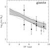 |
Fig. 5 Like Fig. 4 but for luminosity class III stars (giants). |
| In the text | |
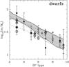 |
Fig. 6 Like Fig. 4 but for luminosity class V stars (dwarfs). |
| In the text | |
|
Fig. A.1 Panel A: mass evolution over 4 Myr for a 85 M⊙ (solid line) and a 120 M⊙ star (dotted line) from literature data (Meynet & Maeder 2003). The dashed line shows a 100 M⊙ star interpolated from the two models. Panel B: luminosity evolution over 4 Myr for the same three stars as in the panel A. Panel C: radius evolution over 4 Myr for the same three stars as in panel A. Panel D: effective temperature evolution over 4 Myr for the same three stars as in panel A. |
| In the text | |
Current usage metrics show cumulative count of Article Views (full-text article views including HTML views, PDF and ePub downloads, according to the available data) and Abstracts Views on Vision4Press platform.
Data correspond to usage on the plateform after 2015. The current usage metrics is available 48-96 hours after online publication and is updated daily on week days.
Initial download of the metrics may take a while.